Article

Impact of Soil Moisture Data Assimilation on Analysis and Medium-Range Forecasts in an Operational Global Data Assimilation and Prediction System

1
Numerical Modeling Center, Korea Meteorological Administration, Seoul 07062, Korea
2
Operational System Development Department, National Institute of Meteorological Sciences, Jeju 63568, Korea
*
Author to whom correspondence should be addressed.
Atmosphere 2021, 12(9), 1089; https://doi.org/10.3390/atmos12091089
Submission received: 30 June 2021 / Revised: 10 August 2021 / Accepted: 20 August 2021 / Published: 24 August 2021
(This article belongs to the Section Atmospheric Techniques, Instruments, and Modeling)

Abstract

:
Accurate initial soil moisture conditions are essential for numerical weather prediction models, because they play a major role in land–atmosphere interactions. This study constructed a soil moisture data assimilation system and evaluated its impacts on the Global Data Assimilation and Prediction System based on the Korea Integrated Model (GDAPS-KIM) to improve its weather forecast skill. Soil moisture data retrieved from the Advanced Scatterometer (ASCAT) onboard the Meteorological Operational Satellite was assimilated into GDAPS-KIM using the ensemble Kalman filter method, and its impacts were evaluated for the 2019 boreal summer period. Our results indicated that the soil moisture data assimilation improved the agreement of the observations with the initial conditions of GDAPS-KIM. This led to a statistically significant improvement in the accuracy of the initial fields. A comparison of a five-day forecast against an ERA5 reanalysis and in situ observations revealed a reduction in the dry and warm biases of GDAPS-KIM over the surface and in the lower- and mid-level atmospheres. The temperature bias correction through the initialization of the soil moisture estimates from the data assimilation system was shown in the five-day weather forecast (root mean squared errors reduction of the temperature at 850 hPa by approximately 5% in East Asia).

1. Introduction

As the lower boundary condition of numerical weather prediction (NWP) models, soil moisture regulates the exchange process of water and energy between land and air on the local, regional, and global scales. Vertically, soil moisture anomalies have effects on the evolution of the surface flux, planetary boundary layer, and free atmosphere [1]. Additionally, it is well-known that there are feedbacks between the soil moisture and atmospheric variables (temperature and precipitation) [2]. Moreover, previous studies have shown that soil moisture affects both the predictability of seasonal forecasts and weather forecasts [1,3,4,5,6,7,8]. For example, Dirmeyer et al. [6] demonstrated that accurate initial soil moisture conditions improved the forecast skill of land surface fluxes, near- surface atmospheric states, and boundary layer properties. Soil moisture anomalies are more persistent over time than those of atmospheric variables [9,10], which are referred to as the soil moisture memory and can contribute to improving weather predictions [6,10,11,12]. Thus, an accurate estimation of the initial soil moisture conditions is essential for the predictability of NWP models.
However, soil moisture is highly variable and depends on the precipitation, land cover, and soil texture [12]. For this reason, a satellite observation with a wide horizontal coverage is more useful than point data by in-situ observations due to coverage and have generally been employed to produce global estimates of soil moisture [13,14]. These include the Advanced Scatterometer (ASCAT) of the European Organization for the Exploitation of Meteorological Satellites’ (EUMETSAT) Meteorological Operational Satellite (MetOp), European Space Agency’s (ESA) Soil Moisture Ocean Salinity (SMOS), Japan Aerospace Exploration Agency’s (JAXA) Global Change Observation Mission Water Shizuku (GCOM-W1), Advanced Microwave Scatterometer Radiometer 2 (AMSR2), and National Aeronautics and Space Administration’s (NASA) Soil Moisture Active Passive (SMAP). Among these satellites, the SMAP retrieval data showed the best skill for estimating the soil moisture [15]. However, ASCAT retrieval data has been used in near-real time to assimilate soil moisture for operational NWP models, such as the Unified Model (UM) of the Met office in the United Kingdom [14] and the Integrated Forecast System (IFS) of the European Center for Medium-Range Weather Forecasts (ECMWF) [16,17]. This demonstrates that ASCAT retrieval data were stably provided in near-real time and represented proper soil moisture quality data with a horizontal resolution appropriate for global NWP models [14].
Remote sensing observations are combined with land surface model (LSM) simulations in space and time to estimate the accurate initial conditions for most soil moisture data assimilations [13,14,17,18,19,20,21,22,23,24,25,26]. It has been proven that soil moisture assimilations using both satellite observations and model simulations produce more accurate soil moisture estimations than those obtained using models or observations only [14,19,20,25,26]. Zheng et al. [24] assessed a soil moisture data assimilation for the National Oceanic and Atmospheric Administration (NOAA) National Centers for Environmental Prediction (NCEP) Global Forecast System (GFS) and demonstrated that the soil moisture assimilation improves the forecast skills of the NWP model in terms of the surface humidity, air temperature, geopotential height, and precipitation.
For the assimilation technique, the soil moisture assimilation systems for the UM and IFS are based on the extended Kalman filter (EKF) [14,17]. Conversely, the ensemble Kalman filter (EnKF) has been employed in NASA’s Land Information System (LIS) for soil moisture data assimilation [18,19,21,24,25]. Reichle et al. [18] argued that EnKF is suitable for the nonlinearities and intermittent characteristics of soil moisture. In addition, they mentioned that the EnKF is more flexible than the EKF for converging errors with increasing the ensemble size. In addition, there is another previous study that conducted soil moisture data assimilation using a local ensemble transform Kalman filter (LETKF), a variant of the EnKF [26]. LETKF is efficient in massive parallel computing because of its unique localization features. Though LETKF is definitely strong in assimilating atmospheric variables with lots of levels, EnKF is feasible for assimilating soil moisture, demanding less computing power and memory.
The Korea Meteorological Administration (KMA) initiated its own NWP model, the Korean Integrated Model (KIM) [27], which began being employed operationally for 10-d weather forecasts in April 2020. KIM was developed to replace the NWP model based on UM and to produce optimal weather predictions for the Korean peninsula. The GDAPS-KIM utilizes a hybrid four-dimensional variational data assimilation (H4DEV) [28] to correct atmospheric initial conditions with real-time observation data, including satellites, radiosondes, global positioning systems, and surface observations. However, it is necessary to develop a soil moisture assimilation system for GDAPS-KIM to provide accurate initial surface conditions.
Thus, in this study, we constructed a soil moisture data assimilation system to improve the weather forecast skill of GDAPS-KIM by correcting the initial surface conditions using satellite observations. Firstly, the system was developed to implement assimilating the ASCAT soil moisture observations using EnKF in the real-time GDAPS-KIM cyclic operational process. Next, we examined the effects of the soil moisture data assimilation on GDAPS-KIM in terms of short- to medium-range time atmospheric predictions by assessing the experiments for the boreal summer season. We attempt to make a decision on the application of the soil moisture data assimilation in GDAPS_KIM and, also, figure out how the corrected initial soil moisture conditions improve the skills of the forecasts in the NWP through these results. This manuscript is structured as follows: Section 2 describes the soil moisture data assimilation system for GDAPS-KIM. Section 3 demonstrates the impact of this system on the initial conditions and forecasts of GDAPS-KIM, and a summary and discussion of our findings are presented in Section 4.

2. Data and Methods

2.1. LSM

In this study, Noah LSM (version 3.3) [29] was used as a stand-alone LSM for soil moisture data assimilation, because KIM’s LSM is based on Noah LSM. In KIM physics packages, the land surface model was developed based on Noah LSM version 3.0, with several modifications [30]. Noah LSM includes the physical processes of soil hydrodynamics [31], penman potential evaporation [32], canopy resistance [33], surface infiltration [34], and subsurface heat flux [35] and consists of four soil layers (0.1, 0.3, 0.6, and 1.0 m). In a previous study [36], Advanced Very-High-Resolution Radiometer (AVHRR) University of Maryland (UMD) land use parameter data were replaced by the Moderate Resolution Imaging Spectroradiometer (MODIS) International Geosphere—Biosphere Program (IGBP), which is used for KIM’s LSM, for the stand-alone LSM. Additionally, the soil moisture is fixed to 1.0 for the glacial region in the stand-alone LSM. Beck et al. [37] mentioned that Noah LSM was almost identical to KIM-LSM, except for calculating the snow amount. Additionally, there could be inherently some differences between the two models, because KIM’s LSM as a coupled model could directly exchange the energy and mass with the atmospheric model. However, a stand-alone Joint UK Land Environment Simulator (JULES) for soil moisture data assimilation was a different version with UM-LSM [38]. The stand-alone Noah LSM will be replaced by stand-alone KIM-LSM that is being constructed.
The stand-alone LSM was spun up for 2007 with 10 consecutive loops, because a previous study demonstrated that a spin-up through 10-year cycles is sufficient for the soil moisture of the LSM to reach equilibrium conditions [36]. Subsequently, a retrospective spin-up was implemented with forcing data from 2008 to 2019. The atmospheric forcing data for the LSM spin-up is the three-hourly Global Land Data Assimilation System forcing data from NASA [39,40], with a horizontal resolution of 0.25°.

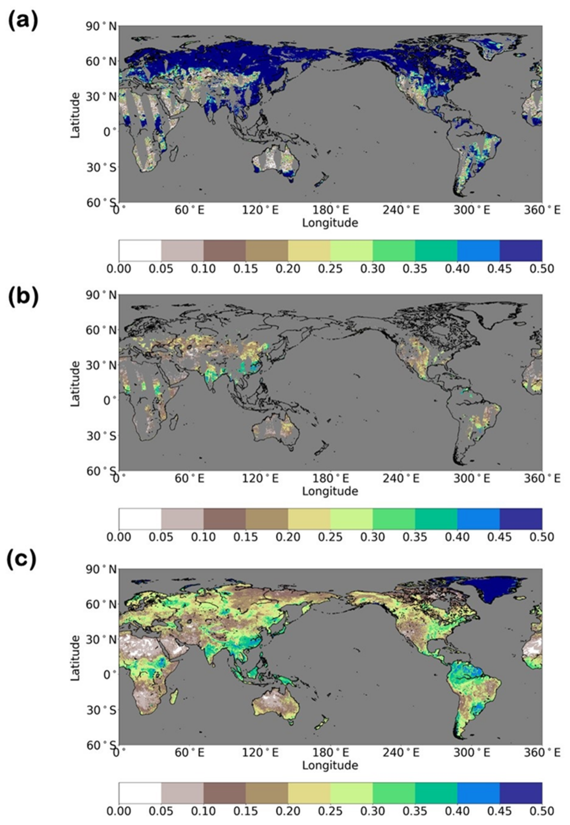
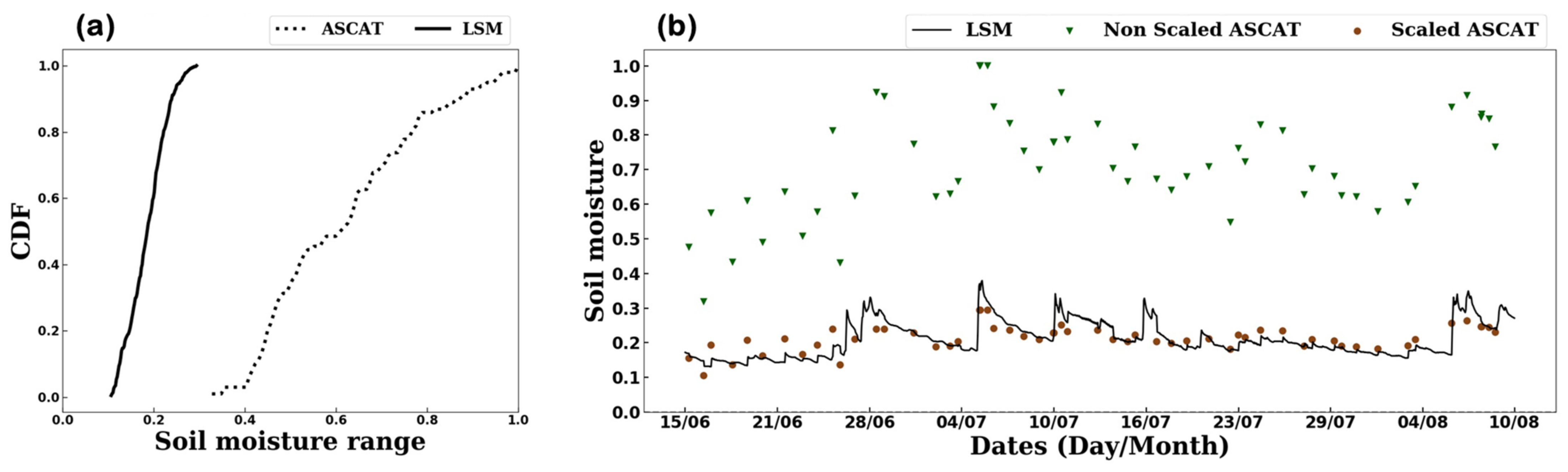
2.2. ASCAT Soil Moisture Data

ASCAT is an active microwave remote sensing instrument with a C-band wavelength of 5.3 GHz. Surface soil moisture data of ASCAT Level-2 products were disseminated in near-real time to allow the NWP centers to use them for data assimilation by EUMETSAT [41]. In this study, ASCAT, which was on-board the first and second meteorological operational (METOP-A and B) satellites, was used. The ASCAT at a 12.5-km swath grid was chosen instead of 25 km, because it has been used for the soil moisture data assimilation of UM [38], and the system we constructed in this study needed high-resolution data for operational KMA global NWP at a 12-km horizontal resolution.
A quality control (QC) process has been implemented to exclude low-quality data where the errors for estimating the ASCAT soil wetness are greater than or equal to 16%. Moreover, the observation data are excluded when the wetland rate exceeds 15%, the complexity of the topology exceeds 20%, or the estimated error is greater than or equal to 16%. In addition, ASCAT data are rejected for freezing temperatures, precipitation, high-density vegetation (i.e., monthly greenness > 70%), or snow cover [14,42]. ASCAT data are also rejected when the MODIS IGBP land cover type belongs to one of the four forest types, including evergreen needle leaf, evergreen broad leaf, deciduous needle leaf, and deciduous broad leaf. Figure 1a,b indicates the ASCAT soil wetness tracks before and after the thinning process, respectively.
The observation error standard deviations for the ASCAT unscaled soil moisture are set to the spatial and temporal constants, 10% (soil wetness index) [20,43]. This value was scaled by the ratio of the soil moisture time series standard deviation of the model to that of the ASCAT soil moisture [25,44].
During the thinning and scaling procedure, the ASCAT soil wetness (Figure 1a) is converted to the volumetric soil moisture, which represents scaled ASCAT soil moisture data (Figure 1b) equivalent to the LSM climate (Figure 1c). In addition, the observation and model prediction should be unbiased towards each other so that the observation biases are corrected before the assimilation is performed using the cumulative density function (CDF) matching method [13,21]. CDF matching is to match the CDF of the ASCAT soil wetness to the CDF of the model’s volumetric soil moisture. To account for the seasonal variability, monthly CDFs were calculated from the soil moisture data of the observations and model simulations during 2016 and 2018. Figure 2 shows the CDF estimates and soil moisture time series of the ASCAT and LSM at 44.625° N, 120.875° E. The CDFs indicate a higher ASCAT soil wetness than the LSM’s volumetric soil moisture (Figure 2a); however, the scaled ASCAT soil moisture is equivalent to the LSM simulation (Figure 2b). In addition, the variability of the scaled values is similar to that of the LSM soil moisture series.

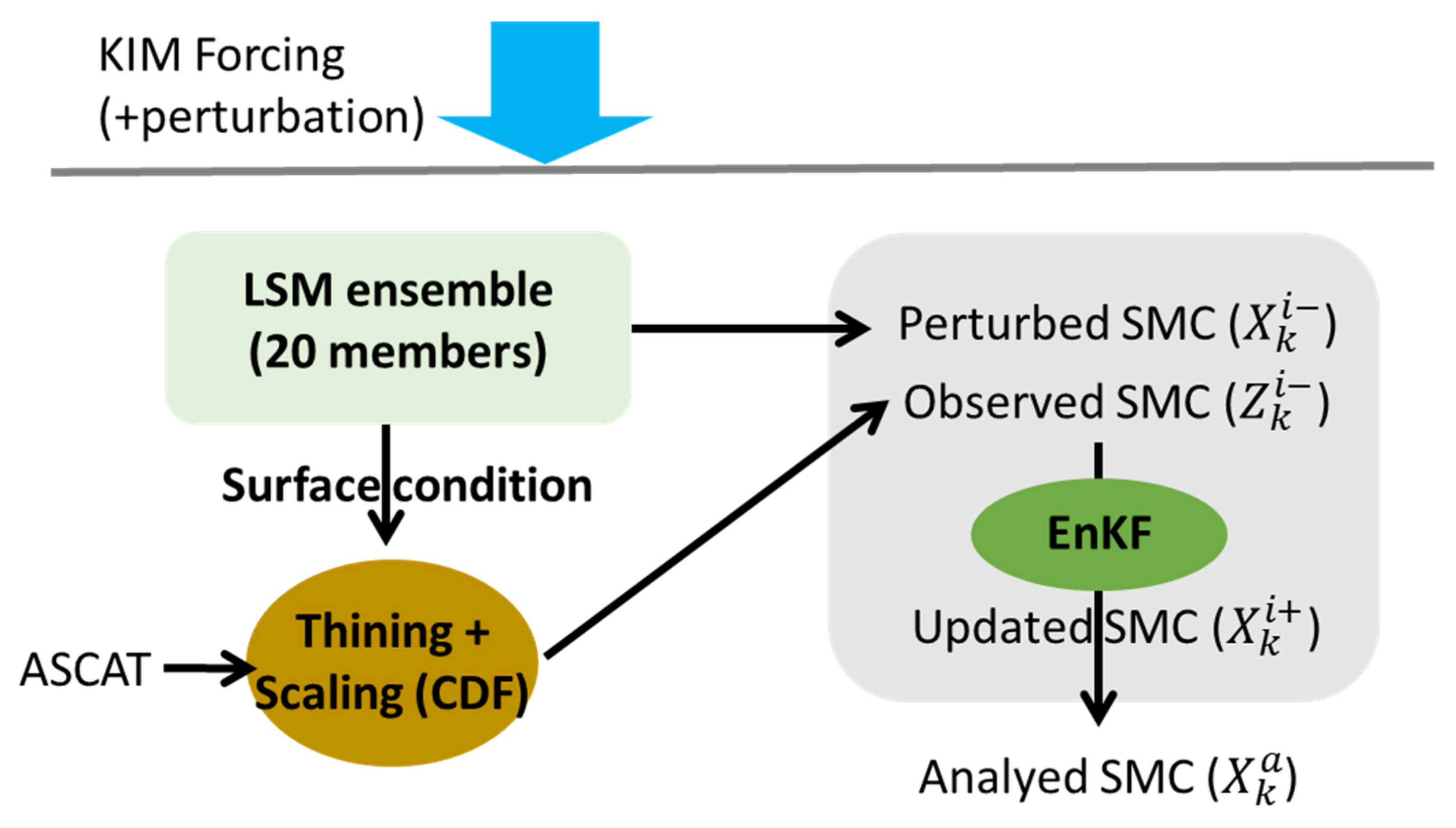
2.3. Data Assimilation Method

An EnKF [18,45] was applied to assimilate the ASCAT observations into GDAPS-KIM. The Kalman filter updates the model state with an observation based on the uncertainty information of the model and the observations. This uncertainty is referred to as the error covariance and is estimated from an ensemble model at the time when the EnKF is updated [46]. The number of ensemble members is 20. The overall soil moisture data assimilation system for GDAPS-KIM is based on LIS version 7.2 (LIS framework, Figure 3) [35,47].
At each time step (t), the ith ensemble model prediction vector ( x t i ) is updated to x t i + by using the observation vector ( z t ), according to Equation (1). In Equation (1), H is the observation operator, and K t is the Kalman gain matrix. The model analysis vector x t a is given by averaging the updated ensemble members (Figure 3).
x t i + = x t i + K t z t H x t i
To produce ensembles in the EnKF, perturbations were applied to the atmospheric forcing variables, indicating the uncertainty of forcing, and the LSM prognostic states, indicating the uncertainty of LSM’s physics and parameters [18,19,45]. The parameters used for generation of the perturbations are described in Table 1, and these are based on previous studies [25,45,48]. Normally distributed additive perturbations with a zero mean were applied to the long-wave radiation and LSM soil moisture, and lognormally distributed multiplicative perturbations with a mean value of 1 were employed for shortwave radiation and precipitation. There was no consideration of the spatial correlation, because we applied one-dimensional EnKF. A first-order regression model (AR1) was used for temporal correlation with time scales of 24 h for the forcing variables and 12 h for the LSM prognostic states. The cross-correlations between the atmospheric forcing variables were employed to represent the physical balance in the atmospheric modeling system. Additionally, the LSM soil moisture variables for each layer were vertically correlated. The nonlinear feature of this perturbation process can make the ensemble background biased. Thus, this unintended perturbation bias was corrected using an unperturbed model simulation [49].

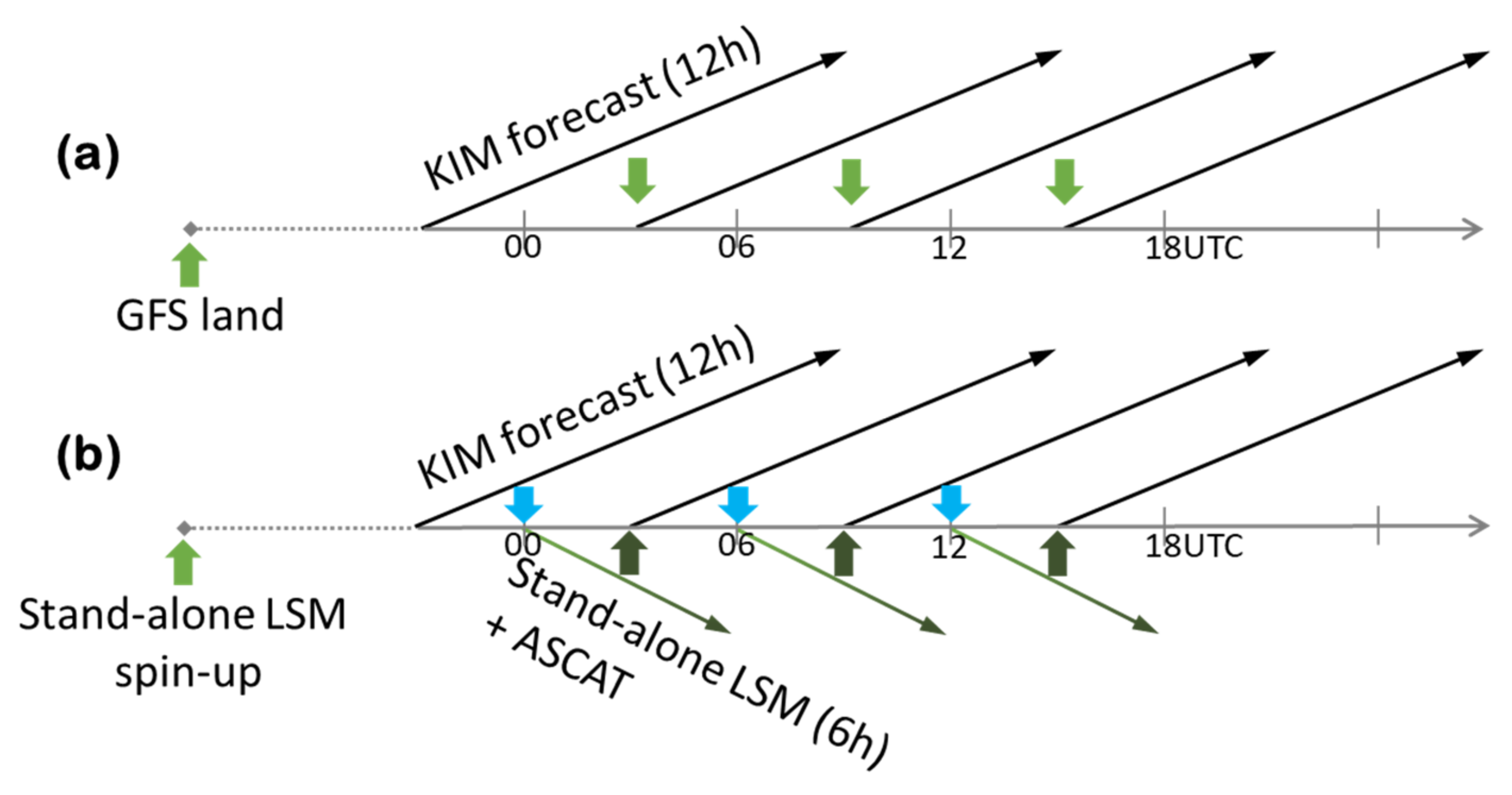
2.4. Model Configuration

The GDAPS-KIM used in this study is a global atmospheric model system, in which a spectral-element nonhydrostatic dynamical core on a cubed sphere grid is used; its horizontal and vertical resolutions are 25 km (12 km in the operational run) and 91 layers (hybrid sigma-pressure coordinate), respectively [27].
To initialize the atmospheric variables, GDAPS-KIM employs H4DEV [28] with LETKF, together with the KIM Package of Observation Processing (KPOP) [50]. GDAPS-KIM assimilates the sonde, surface, aircraft, and satellite observations. Two experiments with (EXP) and without (CTL) soil moisture data assimilation were performed during the boreal summer season. These experiments were initiated with the atmospheric conditions at 00Z 15 June 2019 and then cyclically run using H4DEV.
In the CTL experiment, the land surface condition was initialized at the start using the GFS surface analysis data and then by the model background surface conditions every 6 h during the cycling run (Figure 4a). Conversely, the EXP land surface conditions were initialized using the soil moisture data assimilation system implemented in this study, which was conducted for 6 h at 00, 06, 12, and 18 Z cycles (Figure 4b). GDAPS-KIM was performed for five-day forecasts at 00 and 12 Z cycles from 1 July 2019 to 10 August 2019.

3. Results

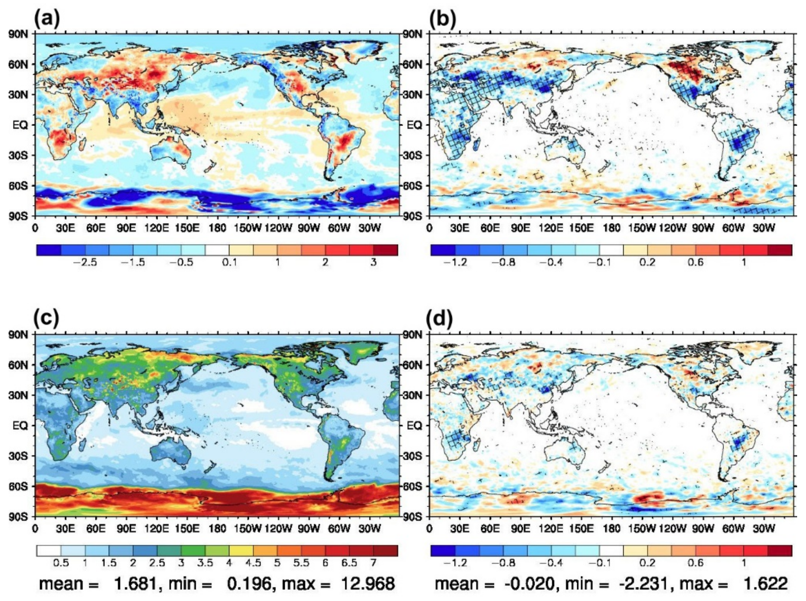
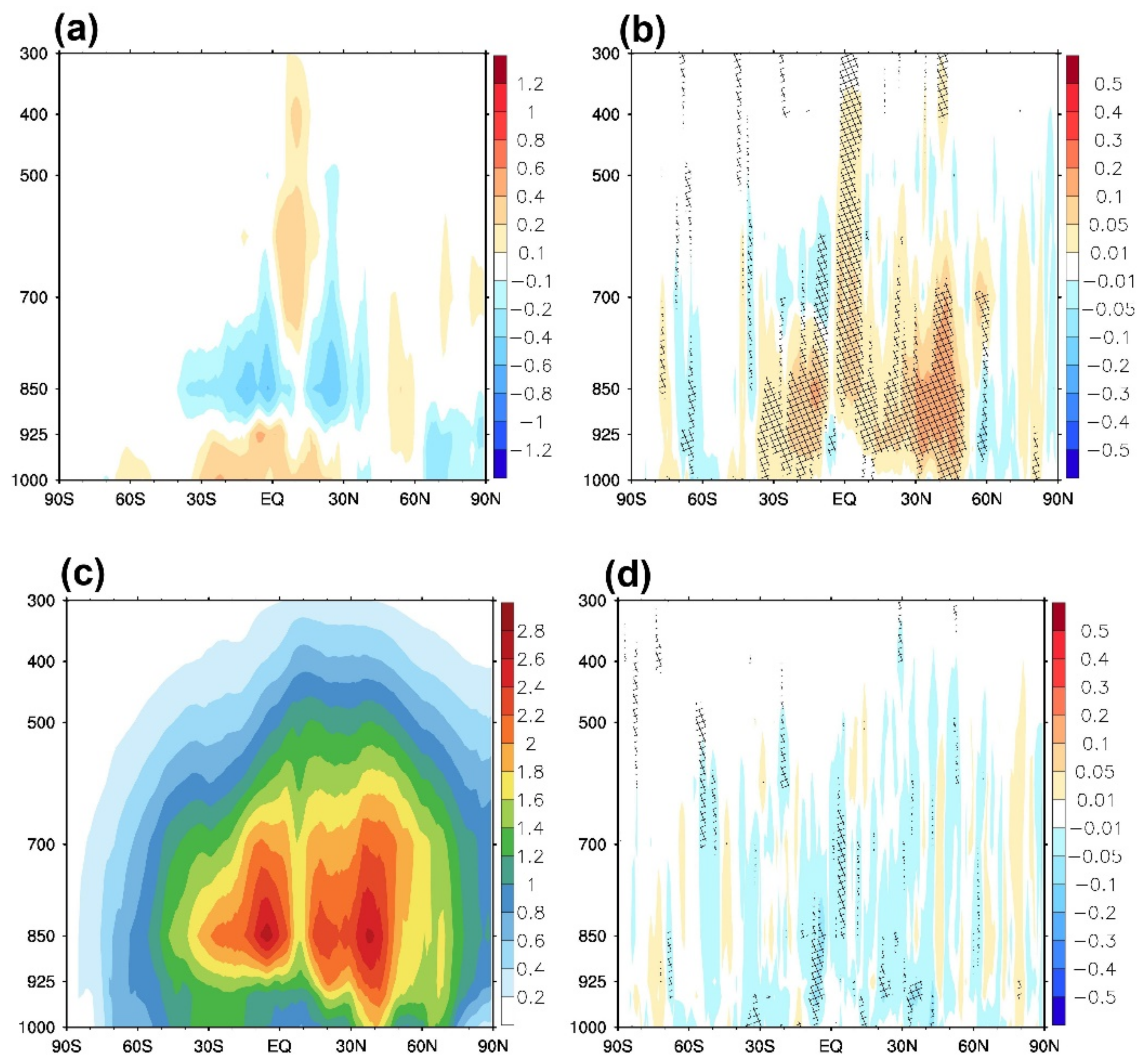
3.1. Effects on Analysis Field

The soil moisture analysis fields from the EXP and CTL experiments were compared with each other and with those from the Soil Moisture Operational Product System (SMOPS) at NOAA, which is produced by using blended multi-satellite soil moisture data. The correlation coefficients were then determined to assess the skills required for analyzing the soil moisture in the experiments [25,51]. The anomaly values of the soil moisture analysis were computed by subtracting the period averages from the analysis values, according to the various climate regions [52]. In this climate region classification, tropical climates are the zone where the monthly mean temperature of the coldest month is higher than or equal to 18 °C, and temperate climates are the zone where the monthly mean temperature of the coldest month is higher than 3 °C and less than 18 °C. The correlation coefficients in the tropical (0.792) and temperate (0.615) regions between the EXP and SMOPS were higher than those (0.351 and 0.130) between the CTL and SMOPS (Table 2). In particular, the correlation coefficient of the EXP in the temperate region was statistically significant, but the correlation coefficient of the CTL was not.
Figure 5 shows the biases of CTL against the ECMWF fifth reanalysis (ERA5) [53] and the differences in the soil moisture analysis between the EXP and the CTL for the first soil layer and the third soil layer. The first soil layer’s depths are 0.1 m and 0.07 m for Noah LSM and for ERA5, respectively, and the third soil layer’s depth is 1.0 m (upper root zone). The second and fourth soil layers were similar to the first and third soil layers, respectively. For the first soil layer, the CTL was drier than ERA5, except for arid areas (Figure 5a). The EXP was wetter than the CTL in most regions of Eurasia, South Africa, and America (Figure 5b). Conversely, the EXP was drier in several arid and high-latitude regions (from 50° N to 60° N) in North America (i.e., Western Canada). For the third soil layer, CTL’s dry biases were larger than the first soil layer, particularly in the Brazilian highlands (Figure 5c). The shrinking of the CTL’s wet bias areas was seen, but the wet biases were larger at the third soil layer. EXP alleviated CTL’s dry biases in East Asia, Eastern Europe, South Africa, the Central United States, and the Brazilian highlands, but the CTL’s dry biases were worse in Western Canada in EXP (Figure 5d).
These soil moisture differences affected the atmospheric analysis fields in the lower troposphere of the model. Figure 6 compares the 2-m specific humidity biases and root mean squared errors (RMSE) against ERA5 between the EXP and CTL experiments. A paired t-test was used to estimate whether the forecasts or errors from the two experiments were significantly different. This t-test is generally useful for two correlated samples [54]. Overall, a dry bias was dominant in the CTL experiment for 2-m-specific humidity, except for the region from 50° N to 60° N in Eurasia and Eastern and Northwest North America (Figure 6a). However, the EXP reduced the CTL’s dry biases and RMSEs in the dry biased regions (Figure 6b,d). These regions were identical to those where the EXP was wetter than the CTL for the soil moisture field (Figure 5b). This result was attributed to more moisture being supplied in the EXP from the surface to the lower atmosphere and was particularly prominent in Asia from 30° N to 50° N, Africa, and South America from 0° E to 30° N. Moreover, this result was statistically significant at the 95% confidence level. In contrast, it was not apparent whether the wet biased regions in the CTL were improved in the EXP (Figure 6d).
The CTL shows warm biases for 2-m air temperatures for the Eurasian continent (predominant over latitudes higher than 30° N), Africa (except for the Sahara Desert), and South America (0° E to 30° S), corresponding to dry biases (Figure 7a). Moreover, the mid-eastern part of North America and the Australian continent were warmer than ERA5. Overall, the warm biased regions were mostly consistent with the dry biased regions. In these areas, which comprised tropical and temperate regions, the EXP was cooler than the CTL, resulting in reduced RMSEs (Figure 7b,d). This is because increased soil moisture strengthens the latent heat flux and weakens the sensible heat flux from the ground to the lower atmosphere [3,12].

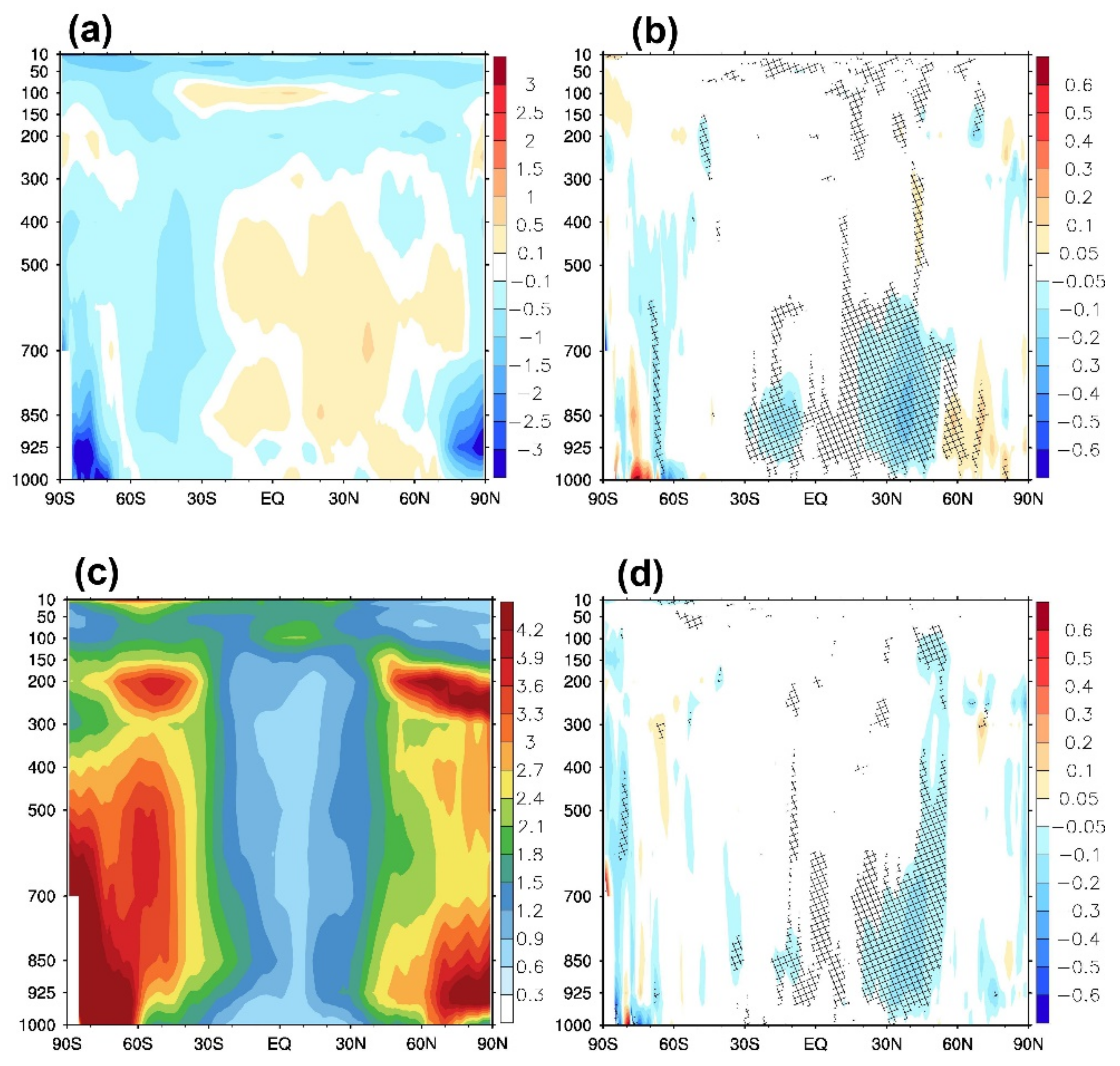
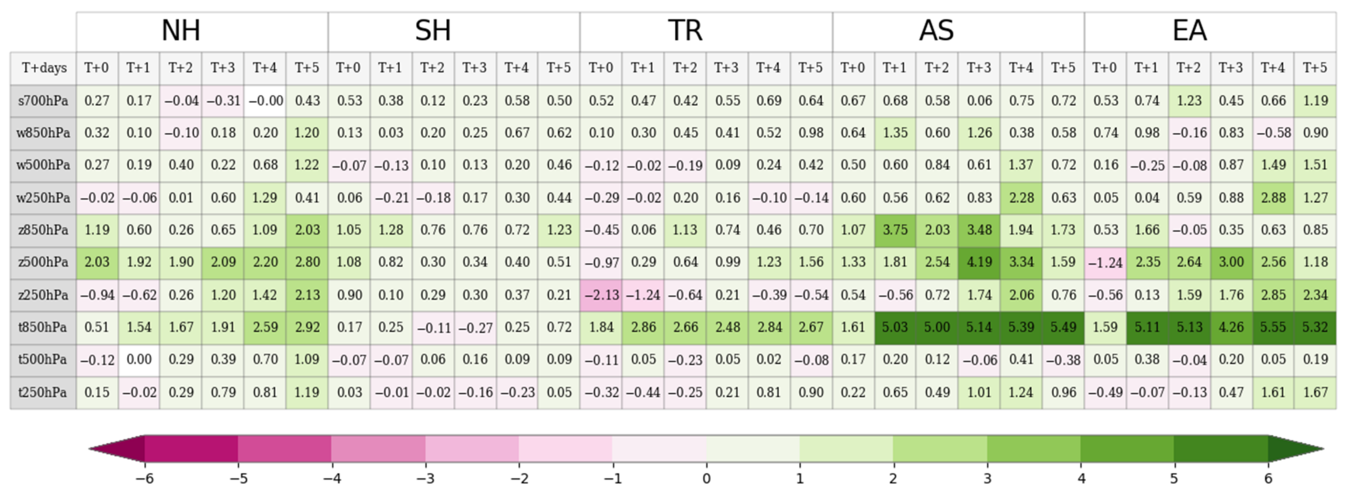
3.2. Effects on Forecast Field

The prediction of the NWP model at the mid-range period provides valuable information for weather forecasting. Changes in the analysis fields via soil moisture data assimilation affect the forecast field. For the 2-m-specific humidity and temperature, the effects of soil moisture assimilation on a five-day forecast were consistent with the analysis fields but were larger. In the EXP, dry biases at the 2-m-specific humidity and warm biases at the 2-m temperature were reduced by soil moisture assimilation, and the RMSEs also decreased (Figure 8b,d and Figure 9b,d). These improvements were statistically significant. Owing to the memory characteristics of soil moisture, improvements in the dry and warm biases in a near surface could accumulate [10]. The EXP wetter regions in 2-m humidity than the CTL were similar to wetter regions in soil moisture at the third soil layer (Figure 5d) in East Asia, Eastern Europe, South Africa, the Central United States, and the Brazilian highlands. For example, it is noticeable that CTL’s large, dry biases of 2-m humidity, indicating large RMSEs, grew from the analysis field (Figure 6a,c) in the Brazilian highlands (Figure 8a,c). These biases might be caused from drier soil moisture conditions from the third soil layer (Figure 5c). Additionally, it was likely that there was feedback between the CTL’s dry biases (Figure 8a,c) and dry biases (Figure 9a,c) [2], but further analysis would be required to figure out it. However, it looks manifest that EXP intensely lessened CTL’s dry biases and RMSEs of 2-m humidity (Figure 8b,d) and warm biases (Figure 9b,d) by providing wetter soil moisture conditions (Figure 5b,d).
In addition to the near-surface variables, we analyzed the vertical profiles of the atmospheric variables to examine how changes in the near surface would be translated into the lower troposphere and above. The CTL indicated dry biases for a specific humidity at the five-day forecast time in the lower and mid-atmospheric levels from 30° S to 50° N (Figure 10a). Moreover, the EXP lessened the dry biases and RMSEs in the regions at the 95% confidence level because of the increased moisture transported from the surface (Figure 10b,d). More moisture from the surface would suppress the sensible heat flux and increase the latent heat flux, which correspond to a reduction in the warm biases (Figure 11b,d). The temperature improvement in the EXP also significantly improved the geopotential height in the lower and mid-levels from 30° S to 50° N (not shown). EXP increased the wet biases at 1000 hPa to 925 hPa in the tropical region but the EXP’s RMSEs were reduced. This means that the CTL’s errors have a larger variation than the EXP.
The overall skill scores of the atmospheric forecasts are displayed in a scorecard in Figure 12 [55], which indicates whether the performance of EXP is better (RMSE reduction; green color) or worse (RMSE increase; purple color) than that of the CTL against the ERA5 reanalysis at each forecast time. Table 3 defines the areas for the scorecards [56]. It is noticeable that the cells representing an improvement in the EXP (indicated by green colors) were dominant in the Northern Hemisphere, Asia, and East Asia at a specific humidity of 700 hPa and wind speed, geopotential height, and temperature of 850 hPa, 500 hPa, and 250 hPa, respectively. Moreover, the improvement rates tended to increase with the forecast time. Among these variables, the temperature at 850 hPa and the geopotential at 500 hPa showed significant improvements. The improvement rates at the five-day forecast were 2.92%, 5.49%, and 5.32% for the temperature at 850 hPa and 2.80%, 3.34%, and 1.18% for the geopotential height at 500 hPa in the Northern Hemisphere, Asia, and East Asia, respectively. However, several degradation cells (mostly > −1%) and neutrality were observed, except for the improvement metrics.
ERA5 reanalysis data, though, are useful for verifying the NWP model forecasting skills; ERA5, like other reanalysis datasets, could have uncertainty, especially in the near-surface variables [57,58,59,60,61]. Thus, we also analyzed the five-day forecasts of the experiments with the surface synoptic weather station network (SYNOP) observation data to ensure a robust verification. The SYNOP datasets are collected by the Global Telecommunication System, and the model forecast results were interpolated horizontally and vertically to the observation space, detailed in Lee et al. [62]. The evaluation results matched well with those against ERA5 in land. For a near-surface-specific humidity, the CTL was drier than the surface observations for most of the land surfaces, except for several parts of the Eurasian continent and North America from 50° N to 60° N and the Australian continent (Figure 13a). The EXP significantly reduced the dry biases and RMSEs in the dry bias region of the CTL (Figure 13b,d). Conversely, the EXP produced mixed effects on the wet bias region of the CTL. Moreover, the warm bias in the CTL was accompanied by a dry bias in the CTL for the land from 30° N to 50° N in Asia, and from 0 °E to 30 °S in Africa and South America (Figure 14a); the warm bias and RMSE in these regions were reduced in the EXP (Figure 14b,d). In Western Canada, a warm bias was accompanied by a wet bias in the CTL. In this region, the EXP was drier than the CTL, and it made the EXP warmer. Thus, there might be another factor for a warm bias for Western Canada, except for soil moisture in the CTL.
The diurnal cycles of the near-surface specific humidity and air temperature were analyzed at 44.57° N and 120.9° E for an approximate five-day forecast (Figure 15). The CTL was drier than the surface observations (Figure 15a). However, the EXP did lessen (8.5% at 12Z cycle) the dry bias of the CTL. Moreover, the daytime improvement in the EXP was more significant than that at night. In addition to the bias reduction, the EXP indicated an improved performance in predicting the diurnal cycles of a specific humidity than that of the CTL. The near-surface temperature in the CTL was higher than the observation temperature during the daytime (Figure 15b), and this bias was attributed to excessive sensible heating from the surface in the CTL. Corresponding to a specific humidity bias reduction, the EXP reduced the CTL warm bias (5.0% at the 12Z cycle); however, the temperature bias of the EXP was similar to that of the CTL at night when the cooling effect was dominant.
Figure 16 and Figure 17 present all the sites average at a 10° interval longitude in the land from 30 °N to 50 °N. If the number of sites was less than thirty, the mean value was not calculated. The variation of the near-surface-specific humidity clearly showed dry biases of the CTL and improvement of the EXP in Eurasia at almost the five-day forecast. The model forecasts at 120 h were averaged for the 00 and 12 UTC target times Figure 16a,c and Figure 17a,c), and the ones at 114 h were averaged for 06 and 18 UTC (Figure 16b,d and Figure 17b,d). EXP lessened the dry biases of the CTL and predicted a more similar near-surface-specific humidity to the observation than the CTL (Figure 16). Corresponding to the dry bias, there were the CTL’s warm biases in variations of the near-surface temperature according to the longitude for Eurasia (Figure 17). The EXP decreased the CTL’s warm biases in Eurasia. However, the magnitude of the CTL’s dry biases in North America were not as large as the ones in Eurasia, and there were wet biases at 00 UTC in Eastern North America (Figure 16). Additionally, the differences between the EXP and CTL in North America were smaller. The CTL showed warm biases in Western North America and mixture bias patterns in Eastern North America (Figure 17). The EXP and CTL showed similar forecasts for the near-surface air temperatures in this region.

4. Summary and Discussion

In this study, we constructed a global soil moisture data assimilation system for GDASPS-KIM to improve its weather forecast skill and examined the impact of soil moisture data assimilation on GDAPS-KIM during the boreal summer season. In the soil moisture data assimilation system, the ASCAT soil moisture observations were assimilated every six hours using EnKF to improve the initial land surface conditions of GDAPS-KIM. Two experiments with and without soil moisture data assimilation were conducted for the period of 00Z 1 July 2019 to 12Z 10 August 2019.
For the initial fields, the soil moisture data assimilation (0.792 and 0.615) showed higher temporal correlation coefficients than those (0.351 and 0.130) without it in the tropical and temperate regions (compared to the SMOPS observations). In addition, the soil moisture content in Eurasia, South Africa, and America increased, which affected the low tropospheric initial fields. Compared to the ERA5 reanalysis fields, it statistically significantly reduced the dry biases and RMSEs in Asia from 30° N to 50° N and in Africa and South America from 0° S to 30° S. This result was attributed to a greater soil moisture supply from the ground, owing to soil moisture data assimilation. Corresponding to the dry biases, the experiment with the soil moisture data assimilation significantly reduced the warm biases and RMSEs of GDAPS-KIM. An augmented moisture content, which was associated with soil moisture data assimilation, would increase the latent heat flux and weaken the sensible heat flux from the surface to the lower atmosphere [12].
The influence of soil moisture data assimilation on a five-day weather forecast was also examined and compared to the ERA5 reanalysis fields. Soil moisture data assimilation decreased the temperature biases and RMSEs in similar regions, thereby positively impacting the initial field. Moreover, the magnitude of the improvement in the five-day forecast was stronger than that in the initial field. The effects of the realistic initial soil moisture conditions were accumulated because of the soil moisture memory characteristics. Specifically, the EXP’s reduction for the five-day forecast was larger than the analysis field in the dry and warm errors of the CTL over the near surfaces in East Asia, Eastern Europe, South Africa, the Central United States, and the Brazilian highlands, where the soil moisture conditions were wetter than the CTL, especially in the third soil layer (root-zone). Ma et al. [63] and Jun et al. [64] also showed that the soil moisture was the cause of the 2-m air temperature over the Central United States and Asia for the five-day forecast in the NWP models in the boreal summer. However, employing ground observations would be needed for the robust evaluation. As shown in the zonally mean fields, GDAPS-KIM produced a dry bias and warm bias in the lower and mid-levels from 30° S to 50° N. However, the soil moisture data assimilation significantly decreased the biases and RMSEs of the specific humidity and temperature at the 95% confidence level.
It is evident from the scorecard, wherein the GDAPS-KIM forecast performance is indicated with a lead time, that the positive impact of soil moisture data assimilation is dominant in the Northern Hemisphere, Asia, and East Asia. It is remarkable that the positive impact tended to rise, along with the forecast period. This was likely because of soil moisture memory explained above. The soil moisture data assimilation led to higher forecast capabilities for temperatures at 850 hPa and geopotential heights at 500 hPa in the Northern Hemisphere (2.92% and 2.80%, respectively), Asia (5.49% and 3.34%, respectively), and East Asia (5.32% and 1.18%, respectively).
In conclusion, incorporating the soil moisture assimilation contributes to improving the initial surface condition and predictability of GDAPS-KIM during the boreal summertime. In particular, the soil moisture data assimilation alleviated the warm biases that are related to soil moisture and enhanced the weather forecasting. It demonstrated that soil moisture assimilation with satellite observation could improve not only the initial surface soil moisture conditions but the weather forecast skills through land–air interactions, as in previous studies [1,3,4,5,6,7,8,24,26]. Based on these results, this assimilation system has been operational for the GDAPS-KIM at KMA since October 2020.
In a future work, another satellite product will be employed to further improve the quality of the initial soil moisture conditions. There are several satellite sensor products for soil moisture described above, but we will choose the one that can be constantly provided in near-real time.

Author Contributions

S.J. and J.-H.P. conceived and designed the experiments; S.J. performed the experiments; S.J., J.-H.P., H.-J.C. and Y.-H.L. analyzed the results; S.J. wrote the original draft preparation; and Y.-H.L., Y.-J.L., K.-O.B. and H.-S.K. supervised the experiments. All authors have read and agreed to the published version of the manuscript.

Funding

This research was funded by the Development of Numerical Weather Prediction and Data Application Techniques of the Numerical Modeling Center of the KMA, grant number KMA2018-00721.

Institutional Review Board Statement

Not applicable.

Informed Consent Statement

Not applicable.

Data Availability Statement

Not applicable.

Acknowledgments

We acknowledge ECMWF and NASA for access to the ERA5 and GLDAS datasets, respectively. We thank the anonymous reviewers for the improvement of this paper through their constructive and insightful comments.

Conflicts of Interest

The authors declare no conflict of interest.

References

  1. Santanello, J.A., Jr.; Peters-Lidard, C.D.; Kumar, S.V. Diagnosing the sensitivity of local land-atmosphere coupling via the soil moisture-boundary layer interaction. J. Hydrometeorol. 2011, 12, 766–786. [Google Scholar] [CrossRef]
  2. Seneviratne, S.I.; Corti, T.; Davin, E.L.; Hirschi, M.; Jaeger, E.B.; Lehner, I.; Orlowsky, B.; Teuling, A.J. Investigating soil moisture-climate interactions in a changing climate: A review. Earth Sci. Rev. 2010, 99, 125–161. [Google Scholar] [CrossRef]
  3. Fisher, E.M.; Seneviratne, S.I.; Vidale, P.L.; Lüthi, D.; Schär, C. Soil moisture-atmosphere interactions during the 2003 European summer heat wave. Geophys. Res. Lett. 2007, 34, 5081–5099. [Google Scholar] [CrossRef]
  4. Koster, R.D.; Mahanama, S.P.P.; Yamada, T.J.; Gianpaolo, B.; Berg, A.A.; Boisserie, M.; Dirmeyer, P.A.; Doblas-Reyes, F.J.; Drewitt, G.; Gordon, C.T.; et al. Contribution of land surface initialization to subseasonal forecast skill: First results from a multi-model experiment. Geophys. Res. Lett. 2010, 37, L02402. [Google Scholar] [CrossRef] [Green Version]
  5. Dirmeyer, P.A.; Halder, S. Sensitivity of numerical weather forecasts to initial soil moisture variations in CFSv2. Weather Forecast. 2016, 31, 1973–1983. [Google Scholar] [CrossRef]
  6. Dirmeyer, P.A.; Halder, S.; Bombardi, R. On the barvest of predictability from land states in a global forecast model. J. Geophys. Res. Atmos. 2018, 123, 13111–13127. [Google Scholar] [CrossRef]
  7. Seo, E.; Lee, M.I.; Jeong, J.H.; Koster, R.D.; Schubert, S.D.; Kim, H.M.; Kim, D.; Kang, H.S.; Kim, H.K.; MacLachlan, C.; et al. Impact of soil moisture initialization on boreal summer subseasonal forecasts: Mid-latitude surface air temperature and heat wave events. Clim. Dyn. 2019, 52, 1695–1709. [Google Scholar] [CrossRef]
  8. Seo, E.; Lee, M.I.; Schubert, S.D.; Koster, R.D.; Kang, H.S. Investiation of the 2016 Eurasia heat wave as event of the recent warming. Environ. Res. Lett. 2020, 15, 114018. [Google Scholar] [CrossRef]
  9. Delworth, T.L.; Manabe, S. The influence of potential evaporation on the variabilities of simulated soil wetness and climate. J. Clim. 1988, 1, 523–547. [Google Scholar] [CrossRef]
  10. Orth, R.; Seneviratne, S.I. Analysis of soil moisture memory from observations in Europe. J. Geophys. Res. 2012, 117, D15115. [Google Scholar] [CrossRef]
  11. McColl, K.A.; Alemohammad, S.H.; Akbar, R.; Konings, A.G.; Yueh, S.; Entekabi, D. The global distribution and dynamics of surface soil moisture. Nat. Geosci. 2017, 10, 100–104. [Google Scholar] [CrossRef]
  12. Santanello, J.A., Jr.; Dirmeyer, P.A.; Ferguson, C.R.; Findell, K.L.; Tawfik, A.B.; Berg, A.; Ek, M.; Gentine, P.; Guillod, B.P.; Heerwaarden, C.; et al. Land-atmosphere interactions: The LoCo perspective. Bull. Am. Meteorol. Soc. 2018, 99, 1253–1272. [Google Scholar] [CrossRef]
  13. Reichle, R.H.; Koster, R.D. Bias reduction in short records of satellite soil moisture. Geophys. Res. Lett. 2004, 31, L19501. [Google Scholar] [CrossRef] [Green Version]
  14. Dharssi, I.; Bovis, K.J.; Macpherson, B.; Jones, C.P. Operational assimilation of ASCAT surface soil wetness at the Met Office. Hydrol. Earth Syst. Sci. 2011, 15, 2729–2746. [Google Scholar] [CrossRef] [Green Version]
  15. Beck, H.E.; Pan, M.; Miralles, D.G.; Reichle, R.H.; Dorigo, W.A.; Hahn, S.; Sheffield, J.; Karthikeyan, L.; Balsamo, G.; Parlnussa, R.M.; et al. Evaluation of 18 satellite- and model-based soil moisture products using in situ measurments from 826 sensors. Hydrol. Earth Syst. Sci. 2021, 25, 17–40. [Google Scholar] [CrossRef]
  16. Drusch, M.; Scipal, K.; de Rosnay, P.; Balsamo, G.; Andersson, E.; Bougeault, P.; Viterbo, P. Towards at Kalman filter based soil moisture analysis system for the operational ECMWF Integrated Forecast System. Geophys. Res. Lett. 2009, 36, L10401. [Google Scholar] [CrossRef]
  17. de Rosnay, P.; Drusch, M.; Vasiljevic, D.; Balsamo, G.; Albergel, C.; Isaksen, L. A simplified extended Kalman filter for the global operational soil moisture analysis at ECMWF. Q. J. R. Meteorol. Soc. 2013, 139, 1199–1213. [Google Scholar] [CrossRef]
  18. Reichle, R.H.; Walker, J.P.; Koster, R.D.; Houser, P.R. Extended versus ensemble Kalman filtering for land data assimilation. J. Hydrometeorol. 2002, 3, 728–740. [Google Scholar] [CrossRef]
  19. Reichle, R.H.; Koster, R.D.; Liu, P.; Mahanama, S.P.; Jjoku, E.G.; Owe, M. Comparison and assimilation of global soil moisture retrievals from the Advanced Microwave Scanning Radiometer for the Earth Observing System (AMSR-E) and the Scanning Multichannel Microwave Radiometer (SMMR). J. Geophys. Res.-Atmos. 2007, 112, D9. [Google Scholar] [CrossRef]
  20. Draper, C.S.; Reichle, R.H.; De Lannoy, G.J.M.; Liu, Q. Assimilation of passive and active microwave soil moisture retrievals. Geophys. Res. Lett. 2012, 39, L04401. [Google Scholar] [CrossRef] [Green Version]
  21. Kumar, S.V.; Reichle, R.H.; Harrison, K.W.; Peters-Lidard, C.D.; Yatheendradas, S.; Santanello, J.A. A comparison of methods for a priori bias correction in soil moisture data assimilation. Water Resour. Res. 2012, 48, W03515. [Google Scholar] [CrossRef]
  22. de Lannoy, G.J.M.; Rosnay, P.D.; Reichle, R. Soil moisture data assimilation. In Handbook of Hydrometeorological Ensemble Forecasting; Duan, Q., Pappenberger, F., Wood, A., Wood, A., Cloke, H.L., Schaake, J.C., Eds.; Springer: Berlin/Heidelberg, Germany, 2015; pp. 1–43. [Google Scholar]
  23. Kolassa, J.; Reichle, R.H.; Draper, C.S. Merging active and passive microwave observations in soil moisture data assimilation. Remote Sens. Environ. 2017, 191, 117–130. [Google Scholar] [CrossRef]
  24. Zheng, W.; Zhan, X.; Liu, J.; Ek, M. A preliminary assessment of the impact of assimilating satellite soil moisture data products on NCEP Global Forecast System. Adv. Meteorol. 2018, 2018, 1–12. [Google Scholar] [CrossRef] [Green Version]
  25. Kumar, S.V.; Jasinski, J.; Mocko, D.M.; Rodell, M.; Borak, J.; Li, B.; Beaudoing, H.K.; Peters-Lidard, C.D. NCA-LDAS land analysis: Development and performance of a multisensory, multivariate land data assimilation system for the National Climate Assessment. J. Hydrometeorol. 2019, 20, 1571–1593. [Google Scholar] [CrossRef]
  26. Seo, E.; Lee, M.I.; Reichle, R.H. Assimilation of SMAP and ASCAT soil moisture retrievals into the JULES land surface model using the Local Ensemble Transform Kalman Filter. Remote Sens. Environ. 2021, 253, 112222. [Google Scholar] [CrossRef]
  27. Hong, S.-Y.; Kwon, Y.C.; Kim, T.-H.; Kim, J.-E.E.; Choi, S.-J.; Kwon, I.-H.; Kim, J.; Lee, E.-H.; Park, R.-S.; Kim, D.-I. The Korean Integrated Model (KIM) system for global weather forecasting. Asia-Pac. J. Atmos. Sci. 2018, 54, 267–292. [Google Scholar] [CrossRef]
  28. Kwon, I.-H.; Song, H.-J.; Ha, J.-H.; Chun, H.-W.; Kang, J.-H.; Lee, S.; Lim, S.; Jo, Y.; Han, H.-J.; Jeong, H.; et al. Development of an operational hybrid data assimilation system at KIAPS. Asia-Pac. J. Atmos. Sci. 2018, 54, 319–335. [Google Scholar] [CrossRef]
  29. Mitchell, K. The Community Noah Land Surface Model (LSM), User’ Guide; National Centers for Environmental Prediction/Environmental Modelling Center: College Park, MD, USA, 2005. Available online: https://ftp.emc.ncep.noaa.gov/mmb/gcp/ldas/noahlsm/ver_2.7.1/ (accessed on 15 May 2021).
  30. Koo, M.-S.; Baek, S.; Seol, K.-H.; Cho, K. Advances in land surface modeling of KIAPS based on the Noah land surface model. Asia-Pac. J. Atmos. Sci. 2017, 53, 361–373. [Google Scholar] [CrossRef]
  31. Mahrt, L.; Pan, H.A. Two-layer model of soil hydrology. Bound.-Layer Meteorol. 1984, 29, 1–20. [Google Scholar] [CrossRef]
  32. Mahrt, L.; Ek, M. The influence of atmospheric stability on potential evaporation. J. Clim. Appl. Meteorol. 1984, 23, 222–234. [Google Scholar] [CrossRef] [Green Version]
  33. Chen, F.; Mitchell, K.; Shaake, J.; Xue, Y.; Pan, H.; Koren, V.; Duan, Y.; Ek, M.; Betts, A. Modeling of land surface evaporation by four schemes and comparison with FIFE observations. J. Geophys. Res. 1996, 101, 7251–7268. [Google Scholar] [CrossRef] [Green Version]
  34. Schaake, J.C.; Koren, V.I.; Duan, Q.Y.; Mitchell, K.; Chen, F. Simple water balance model for estimating runoff at different spatial and temporal scales. J. Geophys. Res. Atmos. 1996, 101, 7461–7475. [Google Scholar] [CrossRef]
  35. Peters-Lidard, C.D.; Zion, M.S.; Wood, E.F. A soil vegetation-atmosphere transfer scheme from modeling spatially variable water and energy balance processes. J. Geophys. Res. Atmos. 1997, 102, 4303–4324. [Google Scholar] [CrossRef]
  36. Jun, S.; Park, J.-H.; Boo, K.-O.; Kang, H.-S. Analyzing off-line Noah land surface model spin-up behavior for initialization of global numerical weather prediction model. J. Korea Water Resour. Assoc. 2020, 53, 181–191. [Google Scholar]
  37. Beck, E.H.; Jeong, J.H.; Yoon, J.H.; Jeong, Y.H.; Kim, K.M.; Kang, S.H.; Lee, J.H.; Yang, K.H.; Bae, J.K. Investigation of Land-Atmosphere Interaction for Global Prediction System; KMA: Seoul, Korea, 2020; pp. 1–84. [Google Scholar]
  38. Park, J.; Boo, K.O.; Kang, H.S. Constructing Land Data Assimilation Process for High Resolution Global Data Assimilation and Prediction System; Numerical Modeling Center/Korea Meteorological Administration (NMC/KMA): Seoul, Korea, 2018; pp. 1–63. (In Korean)
  39. Rodell, M.; Houser, P.R.; Ambor, U.; Gottschalck, J.; Mitchell, K.; Meng, C.; Arsenault, K.; Cosgrove, B.; Radakovich, J.; Bosilovich, M.; et al. The global land data assimilation system. Bull. Am. Meteorol. Soc. 2004, 85, 381–394. [Google Scholar] [CrossRef] [Green Version]
  40. Rodell, M.; Houser, P.R.; Berg, A.A.; Famiglietti, J.S. Evaluation of 10 methods for initializing a Land Surface Model. J. Hydrometeorol. 2005, 6, 146–155. [Google Scholar] [CrossRef]
  41. Wagner, W.; Hahn, S.; Kidd, R.; Melzer, T.; Bartalis, Z.; Hasenauer, S.; Figa-Saldana, J.; de Rosnay, P.; Jann, A.; Schneider, S.; et al. The ASCAT soil moisture product: A review of its specifications, validation results, and emerging applications. Meteorol. Z. 2013, 22, 5–33. [Google Scholar] [CrossRef] [Green Version]
  42. Al-Yarri, A.; Wigneron, J.-P.; Ducharne, A.; Kerr, Y.H.; Wagner, W.; De Lannoy, G.; Reichle, R.; Al Bitar, A.; Dorigo, W.; Richaume, P.; et al. Global-scale comparison of passive (SMOS) and active (ASCAT) satellite based microwave soil moisture retrievals with soil moisture simulations (MERRA-Land). Remote Sens. Environ. 2014, 152, 614–626. [Google Scholar] [CrossRef] [Green Version]
  43. Dorigo, W.A.; Scipal, K.; Parinussa, R.M.; Liu, Y.Y.; Wagner, W.; de Jeu, R.A.M.; Naeimi, V. Error characterization of global active and passive microwave soil moisture datasets. Hydrol. Earth Syst. Sci. 2010, 14, 2605–2616. [Google Scholar] [CrossRef] [Green Version]
  44. Kumar, S.V.; Peters-Lidard, C.D.; Mocko, D.; Reichle, R.; Liu, Y.; Arsenault, K.R.; Xia, Y.; Ek, M.; Riggs, G.; Livneh, B.; et al. Assimilation of remotely sensed soil moisture and snow depth retrievals for drought estimation. J. Hydrometeorol. 2014, 15, 2446–2469. [Google Scholar] [CrossRef]
  45. Reichle, R.H.; Crow, W.T.; Keppenne, C.L. An adaptive ensemble Kalman filter for soil moisture data assimilation. Water Resour. Res. 2008, 44, W03423. [Google Scholar] [CrossRef]
  46. Evansen, G. Sequential data assimilation with a non-linear quasi-geostrophic model using Monte Carlo methods to forecast error statistics. J. Geophys. Res. 1994, 99, 10143–10162. [Google Scholar] [CrossRef]
  47. Kumar, S.V.; Peters-Lidard, C.D.; Tian, Y.; Houser, P.R.; Geiger, J.; Olden, S.; Lighty, L.; Eastman, J.L.; Doty, B.; Dirmeyer, P.; et al. Land Information System: An interoperable frame work for high resolution land surface modeling. Environ. Model. Softw. 2006, 21, 1402–1415. [Google Scholar] [CrossRef]
  48. Kumar, S.V.; Dong, J.; Peters-Lidard, C.D.; Mocko, D.; Gómez, B. Role of forcing uncertainty and background model error characterization in snow data assimilation. Hydrol. Earth Syst. Sci. 2017, 21, 2637–2647. [Google Scholar] [CrossRef] [Green Version]
  49. Ryu, D.; Crow, W.T.; Zhan, X.; Jackson, T.J. Correcting unintended perturbation biases in hydrologic data assimilation. J. Hydrometeorol. 2009, 10, 734–750. [Google Scholar] [CrossRef]
  50. Kang, J.-H.; Chun, H.-W.; Lee, S.; Ha, J.-H.; Song, H.-J.; Kwon, I.-H.; Han, H.-J.; Jeong, H.; Kwon, H.-N.; Kim, T.-H. Development of an observation processing package for data assimilation in KIAPS. Asia-Pac. J. Atmos. Sci. 2019, 54, 303–318. [Google Scholar] [CrossRef]
  51. Liu, Q.; Reichle, R.H.; Bindlish, R.; Cosh, M.H.; Crow, W.T.; de Jeu, R.; de Lannoy, G.J.M.; Huffman, G.J.; Jackson, T.J. The contributions of precipitation and soil moisture observations to the skill of soil moisture estimates in a land data assimilation system. J. Hydrometeorol. 2011, 12, 750–765. [Google Scholar] [CrossRef]
  52. Kotter, M.; Grieser, J.; Beck, C.; Rudolf, B.; Rubel, F. World map of the Köppen-Geiger climate classification updated. Meteorol. Z. 2006, 15, 259–263. [Google Scholar] [CrossRef]
  53. Hersbach, H.; Bell, B.; Berrisford, P.; Hirahara, S.; Horanyi, A.; Muñoz-Sabater, J.; Nicolas, J.; Peubey, C.; Radu, R.; Schepers, D.; et al. The ERA5 global reanalysis. Q. J. R. Meteorol. Soc. 2020, 146, 1999–2049. [Google Scholar] [CrossRef]
  54. Gilleland, E. Confidence Intervals for Forecast Verification: Practical Considerations; National Center for Atmospheric Research: Boulder, CO, USA, 2010. [Google Scholar]
  55. Bush, M.; Allen, T.; Bain, C.; Boutle, I.; Edwards, J.; Finnenkoetter, A.; Franklin, C.; Hanley, K.; Lean, H.; Lock, A.; et al. The first Met Office unified model-JULES regional atmosphere and land configuration, RAL1. Geoscientific Model Development. Geosci. Model. Dev. 2020, 13, 1999–2029. [Google Scholar] [CrossRef] [Green Version]
  56. World Meteorological Organization (WMO). Manual on the Global Data-Processing and Forecasting System; WMO: Geneva, Switzerland, 2019; pp. 1–148. [Google Scholar]
  57. Boisvert, L.N.; Wu, D.L.; Vihma, T.; Susskind, J. Verificaiton of air/surface humidity differences from AIRS and ERA-Interim in support of turbulent flux estimation in the Arctic. J. Geophys. Res. Atmos. 2015, 120, 945–963. [Google Scholar] [CrossRef]
  58. Boilley, A.; Wald, L. Comparison between meteorological reanalyses from ERA-Interim and MERRA and measurements of daily solar irradiation at surface. Renew. Energy 2015, 75, 135143. [Google Scholar] [CrossRef]
  59. Huang, Y.; Dong, X.; Xi, B.; Dolinar, E.K.; Stanfield, R.E.; Qiu, S. Quantifying the uncertainties of reanalyzed Arctic cloud and radiation properties using satellite surface observations. J. Clim. 2017, 30, 8007–8029. [Google Scholar] [CrossRef]
  60. Stengel, M.; Schlundt, C.; Stapelberg, S.; Sus, O.; Eliasson, S.; Willén, U.; Meirink, J.F. Comparing ERA-Interim clouds with satellite observations using a simplified satellite simulator. Atmos. Chem. Phys. 2018, 18, 17601–17614. [Google Scholar] [CrossRef] [Green Version]
  61. Tang, W.; Qin, J.; Yang, K.; Zhu, F.; Zhou, X. Does ERA5 outperform satellite products in estimating atmospheric downward longwave radiation at the surface? Atmos. Res. 2021, 252, 105453. [Google Scholar] [CrossRef]
  62. Lee, E.-H.; Choi, I.-J.; Kim, K.-B.; Kang, J.-H.; Lee, J.; Lee, E.; Seol, K.-H. Verification of the global numerical weather prediction using SYNOP surface observation data. Atmosphere 2017, 27, 235–249. [Google Scholar]
  63. Ma, H.Y.; Klein, S.A.; Xie, S.; Zhang, C.; Tang, S.; Tang, Q.; Morette, C.J.; Van Weverberg, K.; Petch, J.; Ahlgrimm, M.; et al. Cause: On the role of surface energy budget errors to the warm surface air temperature error over the Central United States. J. Geophys. Res. Atmos. 2018, 123, 2888–2909. [Google Scholar] [CrossRef] [Green Version]
  64. Jun, S.; Park, J.H.; Baek, H.J.; Boo, K.O.; Kang, H.S. Utilization of self-organizing Maps to analyzing systematic bias in numerical model: Surface air temperature forecast of KMA GDAPS. J. Korean Inst. 2018, 28, 601–610. [Google Scholar]
Figure 1. (a) Soil wetness on 1 July 2019 from ASCAT, (b) surface volumetric soil moisture after thinning and scaling the ASCAT soil wetness, and (c) the first soil layer volumetric soil moisture from LSM at an instant time of 00Z 1 July 2019.
Atmosphere 12 01089 g001
Figure 2. (a) CDF estimates of the ASCAT soil wetness (solid line) for July and LSM volumetric soil moisture (dashed line) from 2016 to 2018 at 44.625° N, 120.875° E. For this location: (b) hourly time series of the non-scaled ASCAT soil wetness (green dots) and scaled ASCAT volumetric soil moisture (brown dots) against the stand-alone LSM volumetric soil moisture (black line).
Atmosphere 12 01089 g002
Figure 3. Soil moisture data assimilation system.
Atmosphere 12 01089 g003
Figure 4. GDAPS-KIM soil moisture initialization system (a) without and (b) with soil moisture data assimilation.
Atmosphere 12 01089 g004
Figure 5. Biases in the CTL against ERA5 and EXP minus the CTL difference of the volumetric soil moisture for (a,b) the first soil layer and (c,d) the third soil layer from 15 Jun 2019 to 10 August 2019.
Atmosphere 12 01089 g005
Figure 6. (a) Biases and (c) RMSEs of 2-m-specific humidity in the CTL against the ERA5 reanalysis, and (b) differences in the biases and (d) RMSEs between the EXP and CTL over the period of 1 July 2019 to 10 August 2019 for the analysis field. The hatched regions indicate a difference significant at the 95% confidence level.
Atmosphere 12 01089 g006
Figure 7. (a) Biases and (c) RMSEs of 2-m air temperature in the CTL against the ERA5 reanalysis, and (b) differences in the biases and (d) RMSEs between the EXP and CTL over the period of 1 July 2019 to 10 August 2019 for the analysis field. The hatched regions indicate a difference significant at the 95% confidence level.
Atmosphere 12 01089 g007
Figure 8. (a) Biases and (c) RMSEs of 2-m-specific humidity in the CTL against the ERA5 reanalysis, and (b) differences in the biases and (d) RMSEs between the EXP and CTL over the period of 1 July 2019 to 10 August 2019 for a five-day forecast. The hatched regions indicate a difference significant at the 95% confidence level.
Atmosphere 12 01089 g008
Figure 9. (a) Biases and (c) RMSEs of 2-m air temperature in the CTL against the ERA5 reanalysis, and (b) differences in the biases and (d) RMSEs between the EXP and CTL over the period of 1 July 2019 to 10 August 2019 for a five-day forecast. The hatched regions indicate a difference significant at the 95% confidence level.
Atmosphere 12 01089 g009
Figure 10. (a) Biases and (c) RMSEs of the zonal mean specific humidity in the CTL against the ERA5 reanalysis, and (b) differences in the biases and (d) RMSEs between the EXP and CTL over the period of 1 July 2019 to 10 August 2019 for a five-day forecast. The hatched regions indicate a difference significant at the 95% confidence level.
Atmosphere 12 01089 g010
Figure 11. (a) Biases and (c) RMSEs of the zonal mean air temperature in the CTL against the ERA5 reanalysis, and (b) differences in the biases and (d) RMSEs between the EXP and CTL over the period of 1 July 2019 to 10 August 2019 for a five-day forecast. The hatched regions indicate a difference significant at the 95% confidence level.
Atmosphere 12 01089 g011
Figure 12. Scorecard of the RMSE improvement rates for the specific humidity at 700 hPa (s700 hPa); wind speed at 850 hPa, 500 hPa, and 250 hPa (w850 hPa, w500 hPa, and w250 hPa); geopotential height at 850 hPa, 500 hPa, and 250 hPa (z850 hPa, z500 hPa, and z250 hPa); and temperature at 850 hPa, 500 hPa, and 250 hPa (t850 hPa, t500 hPa, and t250 hPa) in the Northern Hemisphere (NH), Southern Hemisphere (SH), Tropics (TR), Asia (AS), and East Asia (EA) for a five-day forecast.
Atmosphere 12 01089 g012
Figure 13. (a) Biases and (c) RMSEs of near-surface-specific humidity in the CTL against the near-surface observations, and differences in (b) biases and (d) RMSEs between the EXP and CTL for a five-day forecast.
Atmosphere 12 01089 g013
Figure 14. (a) Biases and (c) RMSEs of near-surface air temperature in the CTL against the near-surface observations, and differences in (b) biases and (d) RMSEs between the EXP and CTL for a five-day forecast.
Atmosphere 12 01089 g014
Figure 15. Diurnal cycle of (a) the near-surface-specific humidity and (b) near-surface air temperature at latitude 44.57° N, longitude 120.9° E in the observation and model forecasts (EXP and CTL); the 114-h forecast for the 06, 18Z cycle and 120-h forecast for the 00, 12Z cycle were averaged.
Atmosphere 12 01089 g015
Figure 16. The variations of the near-surface-specific humidity according to the longitude and latitude from 30° N to latitude 50° N in the SYNOP observation and model forecasts (EXP and CTL) at 00 (a), 06 (b), 12 (c), and 18 (d) UTC. The 114-h forecasts for 06 and 18 UTC and 120-h forecasts for 00 and 12 UTC were averaged.
Atmosphere 12 01089 g016
Figure 17. The variations of the near-surface air temperature according to the longitude and latitude from 30° N to latitude 50° N in the SYNOP observation and model forecasts (EXP and CTL) at 00 (a), 06 (b), 12 (c), and 18 (d) UTC. The 114-h forecasts for 06 and 18 UTC and 120-h forecasts for 00 and 12 UTC were averaged.
Atmosphere 12 01089 g017
Table 1. Parameters for generating perturbations to the atmospheric forcing variables and soil moisture of LSM in EnKF. P is precipitation, SW is downward shortwave radiation, LW is downward longwave radiation, and SM1–SM4 are the LSM prognostic soil moisture at the first soil layer to the fourth soil layer.
VariablesPerturbation TypesStandard DeviationsTime Correlations (h)Cross Correlations
PSWLWSM1SM2SM3SM4
PMultiplicative0.5241.0−0.80.5
SWMultiplicative0.324−0.81.0−0.5
LWAdditive50.024−0.50.51.0
SM1Additive0.0112 1.00.60.40.2
SM2Additive0.00612 0.61.00.60.4
SM3Additive0.00312 0.40.61.00.6
SM4Additive0.001512 0.20.40.61.0
Table 2. Correlation coefficients of the volumetric soil moisture in GDAPS-KIM and SMOPS in arid, tropical, and temperate regions during the boreal summer season. The asterisks indicate statistical significance at the 99% confidence level, and no asterisks indicate no statistical significance (under the 90% confidence level).
ExperimentAridTropicalTemperate
EXP0.0750.792 *0.615 *
CTL0.0060.351 *0.130 *
Table 3. Area definitions for calculating the scorecards (Figure 12).
AreasDefinitions
Northern Hemisphere (NH)90° N–20° N, all longitudes
Southern Hemisphere (SH)90° S–20° S, all longitudes
Tropics (TR)20° N–20° S, all longitudes
Asia (AS)25° N–65° N, 60° E–145° E
East Asia (EA)20° N–55° N, 100° E–150° E
Publisher’s Note: MDPI stays neutral with regard to jurisdictional claims in published maps and institutional affiliations.

