1. Introduction
The layers of increased ionization that appear at the heights of the E-region of the ionosphere are called sporadic E layers (E
s layers). These sporadic layers in the E-region, which occur at all latitudes, have been studied for many decades. The majority of the information we possess on E
s layers was obtained by vertical sounding using ionosondes. Currently, E
s layers are being investigated using modern digital ionosondes, lidars, incoherent scatter radars (ISR), very high frequency (VHF) and partial reflection (PR) radars, rocket probes, and signals from GPS and GLONASS navigation satellite systems [
1,
2,
3,
4,
5,
6,
7,
8,
9,
10,
11,
12,
13]. Many important characteristics of the E
s layers are well understood, but continued research is still important, as these layers can significantly affect the propagation of HF and VHF radio waves and provide radio communications in disturbed ionospheric conditions or when reflections from the F layer are not possible.
The E
s layer is a plasma formation with a high degree of ionization, which appears, as a rule, at altitudes of 90–130 km. At 300 m to several km thick, the E
s layer is distinguishable from the other regular D, E, and F layers of the ionosphere. As a rule, E
s layers are a horizontal extension from 20 to 200 km [
14,
15]. Some of them are uniform in the horizontal plane and blanket overlying regions of the ionosphere, while others are semitransparent and consist of ionization clouds (patches). Sporadic E layers can move with a horizontal velocity of 20–130 km/h. Multiple layers may sometimes appear, separated from each other by several kilometers (6–10 km). The E
s layer lifetime can range from several hours to several minutes. Short-lived layers, called transient layers, have been actively studied for the last ten years [
7,
10,
14,
15,
16,
17,
18,
19,
20,
21]. Moreover, sometimes the sporadic E layer begins to form under the action of solar tides in the lower part of the F2 layer at altitudes of about 180 km or in the valley between the E and F layers at altitudes of 120–180 km [
1,
3,
18,
19,
20]. This so-called intermediate E
s layer slowly descends with the downward plasma movement and becomes stable at altitudes of 100–120 km [
3].
Sporadic E events have been studied since the late 1960s, and the main mechanism for their generation is well understood. For example, the formation of sporadic ionization layers at mid-latitudes is explained by the wind shear theory, which is when a vertical shear in a neutral wind collects plasma in the thin ionization layer that can exist for a long time due to long-lived metal ions ([
14,
15,
16,
22,
23,
24,
25,
26] and references therein).
Along with numerous methods for the investigation of sporadic E layers, a method for studying the ionosphere, by creating artificial periodic irregularities (APIs), has been available for many years [
18,
19,
20,
27,
28,
29,
30]. This method for studying the ionosphere and the neutral atmosphere, the API technique, was developed at the Radiophysical Research Institute (Nizhny Novgorod, Russia). The API diagnostics of the ionosphere includes three main stages: the creation of APIs by radiation of a powerful heating facility, the plasma diagnostics by sounding of the created periodic structure with probe radio waves, and the determination of many parameters of the ionosphere and neutral atmosphere based on the measured characteristics of API scattered signals. APIs are generated in the field of the standing electromagnetic wave, which are formed due to interference of the HF radio waves radiated to the zenith and reflected from the ionosphere. APIs are observed at altitudes from 60 km up to the level of the reflection of powerful and probing radio waves in the F-region. Approximately ten methods have been developed for determining the parameters of the ionosphere and neutral atmosphere by this technique. A detailed description of the API technique and diagnostic methods for the ionosphere can be found in [
18]. It became clear through long-term observations that the API technique is a very effective method for studying any sporadic layers, including weak E
s layers, inaccessible to observation by ionosonde, and as well as short-lived (transient) layers [
21]. In
Section 4, we provide some examples of various sporadic events observed by the API technique.
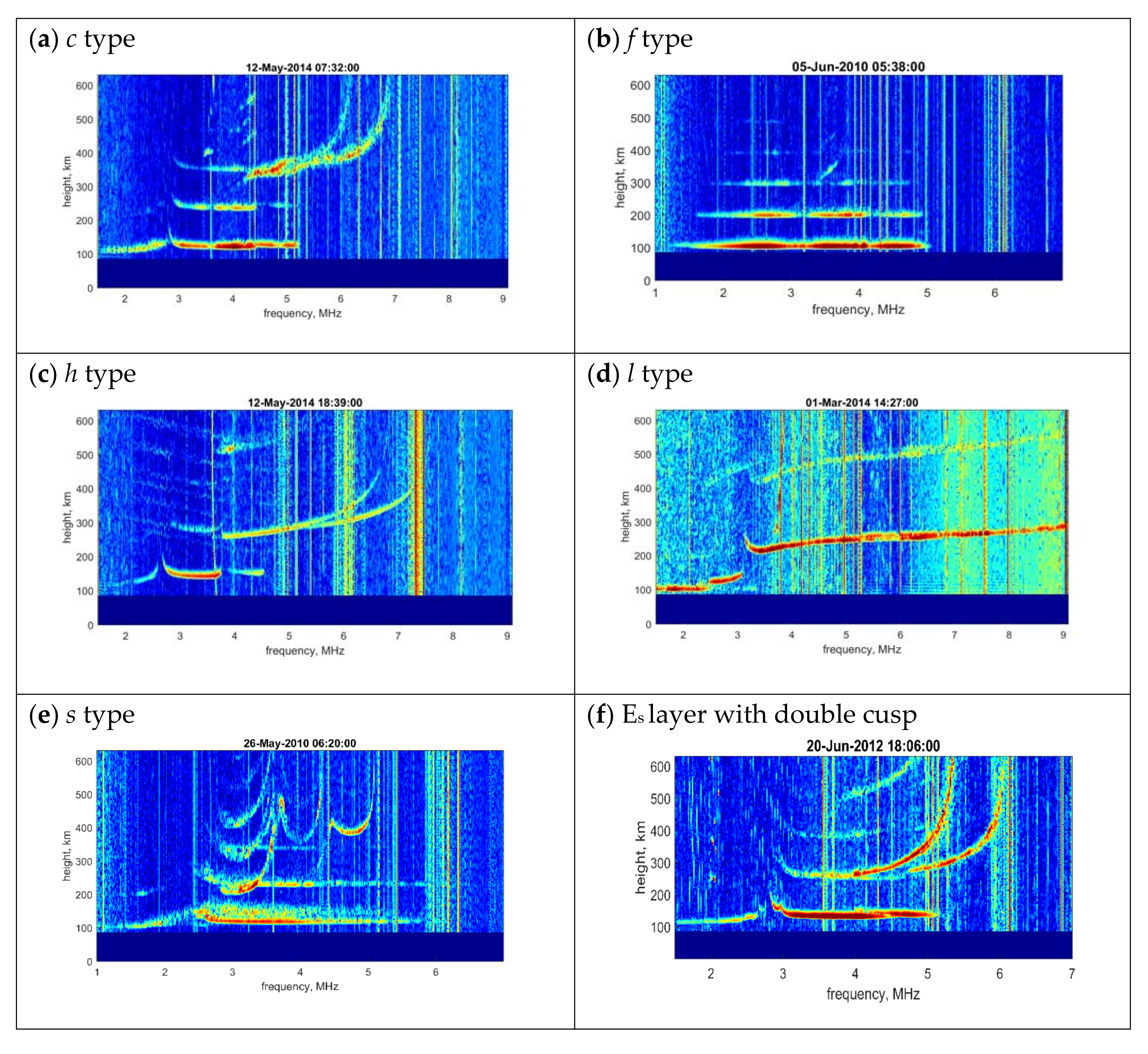
In ionograms, according to the shape of the dispersion delay of the trace of the E
s layer, the following main types are distinguished:
a,
c,
f,
h,
l,
q,
s, and
r [
31]. Type
a (auroral) is usually observed during night hours together with auroras at high latitudes. Type
c (cusp) is most often observed in the daytime and has a peak-like inflection in the frequency range close to the critical frequency of the E layer. The traces in the ionogram from the E
s layer of the
f type are flat and have no visible dispersion delays of the trace. They are often observed at night when there is no background ionization of the E layer. Sporadic layers of this type are also often blanketing. The
h (high) layer type differs from the
c layer type in that it has a discontinuity in height relative to the maximum of the trace from the E layer. Such sporadic layers can perhaps be attributed to the intermediate E
s layers. The type
l (low) layer is similar in shape to the type
f layer, but it is observed in the daytime below the trace from the E layer. Thus, it can be called an “underlayered” E
s. Type
q (equatorial) is observed at equatorial latitudes, as a rule, during daytime hours. These, and other types of sporadic layers, are described in detail in [
31]. The diffuse
s type of E
s layer in ionograms is observed as a “blurred spot” above other E
s trace, and is possibly due to lateral reflections of other nearby E
s layers. A layer of type
r (retardation) has a dispersion delay at the beginning of the trace (as in types
c and
h). This delay increases with increasing frequency and resembles a trace from a regular E layer. In this case, E
s layer traces, showing an increase in virtual height at the high frequency end, are similar to group retardation. Examples of ionograms with such sporadic layers, obtained by Cyclone ionosonde at the Kazan Federal University, are shown in
Figure 1. Sporadic layers typical for mid-latitudes are constantly recorded by the digital ionosonde Cyclone [
8,
21]. Sometimes, unusual ionograms are observed. An example of such an ionogram with a
c type of E
s layer, which has a trace with an unusual double cusp, is shown in
Figure 1f.
For a general overview of the types of Es layers, we have provided brief descriptions, paying special attention to the c type of the Es layer with an unusual trace with a double cusp. From observations of the ionosphere with the Cyclone ionosonde, we observed that a sporadic E layer of c type often exists at the latitude of the ionosonde, especially in the daytime. Likewise, sometimes unusual ionograms of the Es layer of the c type, with a double cusp in the low-frequency part of the trace of the Es layer, are observed. We wanted to determine the reasons for the appearance of such ionograms, and attempted to identify the shape of the altitude profile of the electron density, which provides an unusual trace of the double cusp in the ionogram.
The aim of this work was to analyze and simulate the shape of an unusual E
s trace, which was repeatedly recorded by the Cyclone ionosonde. Such a layer has a double cusp in the low frequency part of the trace, which resembles two steps. An example of an ionogram with a sporadic E layer of this type, obtained at 18:04 LT on 26 May 2010, is shown in
Figure 2. The upper part of the double cusp is marked with a circle. As is shown in
Figure 2, the double cusp in the X-mode is absent due to the greater absorption of the extraordinary wave in the ionosphere. An additional feature of the trace with the double cusp discussed in this article is the presence of a small dispersion delay at the high-frequency end of the trace.
To elucidate on the reason for the appearance of a double cusp, we simulated the configuration of traces in the ionogram for the lower part of the E and Es layers based on the selection of a suitable electron concentration profile.
2. Simulation of the Electron Density Profile of the Es Layer Based on the Real Ionogram and Results
The simulation was carried out on the basis of the ionogram shown in
Figure 2. We selected the electron density profile
N(
h) in such a way that the calculated virtual heights of the ionosonde signals reflected from the ionosphere were in good agreement with the traces on the ionogram, including the double cusp of the E. In other words, as a result of modeling, we wanted to obtain an ionogram similar to that measured by an ionosonde.
First, for the ionogram shown in
Figure 2, we selected the profile of the electron density
N(
h), calculated by the IRI model [
32], shown in
Figure 3. The critical frequency of the E layer was 2.20 MHz according to the ionogram and 2.35 MHz according to the IRI-2016 model. Thus, the shape of the lower part of the
N(
h) profile was close to parabolic, and the critical frequency of the E layer, according to the IRI-2016 model, was close to the critical frequency of the E layer of the real ionogram.
At the next stage, this height profile of the electron density was used to calculate the virtual height of the reflection of the radio wave during vertical sounding. For the refractive index of cold plasma, we used the Appleton-Hartree formula without accounting for collisions [
33,
34]:
where
is the probing frequency;
fH~1.4 MHz is the electron gyro frequency;
fN is the plasma frequency;
B0 is the Earth’s magnetic field intensity and
α is the angle between the vector of the Earth’s magnetic field
and the wave vector
; N is the electron density,
e and
m are the electron charge and mass, respectively; and
is the dielectric constant. The
‘+’ sign in the denominator is used for ordinary mode, and the
‘−’ sign for the extraordinary one.
The virtual reflection height
hv was calculated using the formula:
where
hr is the height and
Nr is the electron density at the level of the wave reflection,
h0 is the height of the beginning of the ionosphere and the electron density,
N0, at this height for the calculation. For the location of the Cyclone ionosonde (55.85° N; 48.8° E), angle α is equal to ~18°.
For the correct calculation of virtual heights, it was necessary to select the
N(
h) profile shape for the E layer and add the E
s layer profile reshape to it. The parabolic shape of the electron density profiles of the main layers of the ionosphere are often used for simulations. However, for the ionogram shown in
Figure 2, the use of the parabolic shape for the E layer was inconvenient due to the fact that it was additionally necessary to select the shape of the profile and the height of the E
s layer in order to clarify the reason for the appearance of the double cusp. With this selection, it was more convenient to use functions that had a lower part that is similar to a parabola and an upper part that is flat and, thereby, more closely corresponds to the sporadic E layer in the ionogram. Several variants of functions suitable for approximating the
N(
h) profile were considered. First, we used a polynomial function in the form
. The lower part of this function also turned out to be difficult to apply to the considered ionogram. The most convenient function was the hyperbolic tangent, shown in
Figure 4. The axis values are given in conventional dimensionless units. Further, a grid of the height and density of the electron concentration was applied to this function so that the model ionogram was similar to the real one. In the large rectangle in
Figure 4, we selected the range of changes in the variables (x,y) of the curve for the shape of the profile of the E layer. We likewise set the upper and lower altitude boundaries of the E layer to correspond with traces on the ionogram. The square shows the variation interval of the variables (x,y) for the model function of the E
s layer profile.
After the E layer profile was selected, the virtual reflection height was calculated based on the hyperbolic tangent function using Equation (2). In this case, the window of the large rectangle and the upper and lower boundaries of the altitude interval changed until the calculated virtual heights became equal to the corresponding heights of the E and Es layers on the ionogram.
3. Results
The simulation result, shown in
Figure 5, is presented in the graph of the selected profile of the electron concentration of the dependence of the virtual heights
h on the frequency
f for the O- and X-modes, obtained from the ionogram in
Figure 2 and calculated by Equation (2), with consideration of the selected altitude profile,
N(
h). It can be seen that the traces obtained as a result of modeling are close to the traces of a real ionogram. The thickening of the profile in the lower part (substrate) of the E
s layer most likely has a downwardly convex parabolic shape, which corresponds to a small dispersion delay at the high-frequency end of the upper cusp trace. The half-thickness of this thickening of the lower part of the E
s layer was ~3.5 km, and the half-thickness of the main E
s layer was ~0.9 km.
The following main result of the simulation can be formulated. It was found that the profile of the lower part of the main layer E
s had a parabolic upward convex shape. However, it was more convenient to use the hyperbolic sine function in the calculations, which were selected by choosing the starting and ending points of the
N(
h) profile curve. If a different shape of the E
s layer profile of the main layer is selected, the calculated reflection traces for the O- and X-modes do not correspond to the traces of the ionogram, including by the type of the observed double cusp. In addition, in this case, the calculated traces of the extraordinary component did not coincide with the traces of the real ionogram. A similar profile of the E
s layer was also given in [
7], where measurements were carried out using EISCAT UHF radar.
4. Discussion
One finding is the assumption of the existence of a double Es layer or the presence of two Es layers with parabolic electron density profiles of a small width. In this case, one (second) layer must have a critical frequency of the upper cusp (main Es layer). However, the simulation showed that the location of the first Es profile, which was lower than the second, gave a lower virtual height than the second layer. When the first layer is located above the second one, it becomes blanketing for the second layer, which will not allow the ionosonde sounding signals to be reflected from the ionosphere.
One can also assume the existence of two Es layers, in differing locations above the observation point, but away from each other within the visibility range of the ionosonde radiation pattern. In this case, the overlapping of the reflected signals from the two layers would occur, and the trace on the ionogram would have the form of scattered reflections. This was not observed. On the contrary, the trace from the Es layer in the ionogram had a smooth transition from the first cusp to the second. Therefore, the assumption made about the thickening of the lower part of the Es layer seems to be correct.
Moreover, the reason for the appearance of a trace similar to that shown in
Figure 2, with a double cusp at the low-frequency end of the E
s layer trace, may be the stratification of the E layer. The valley between the E and F layers is the least explored region of the ionosphere. To a large extent, the valley is controlled by the sun zenith angle and wave processes leading to the formation of multiple E
s layers and the stratification of the E-layer [
3,
4,
13,
17]. We also observed similar layering in the E region, including the E
s layer, through the API technique [
18,
20]. An example of such a complex configuration of the E region is shown in
Figure 6 and
Figure 7. Note that the studies of the ionosphere, including the sporadic E layer, using the API technique are based on the measurement of amplitudes and phases of signals scattered by irregularities at the stage of their relaxation. It is on this basis that we obtain time-height-amplitude plots, similar to those shown in
Figure 6.
In
Figure 6, the dependence of the amplitude of the signal scattered by the API versus the height and time is shown. The scattered signals from the API in the D region (h = 90 km) and from the API in the E layer (90–135 km) are shown. In
Figure 6a,b, relating to the period of a partial sun eclipse on 11 August 1999, multiple stratifications of the D and E regions are clearly visible. The dependences of the scattered signal amplitudes for 12 August 1999 are shown in
Figure 6c,d.
Figure 6c shows the formation of a weak sporadic E layer at an altitude of 134 km (the lower boundary of the layer). In
Figure 6d, scattered signals from two connected E
s layers are visible in the altitude region of 112–123 km.
Figure 7 presents the height profiles of the electron density obtained by the API method. Methods for obtaining the
N(
h) profile are described in detail in [
18].
The left panel of
Figure 7 shows sporadic E
s layers at an altitude of 115 km and an intermediate layer in the valley at an altitude of 145 km. On the right panel, one can see two E
s layers spaced 10 km apart in terms of height.
The examples of phenomena associated with sporadic layers presented in
Figure 6 and
Figure 7 show that unusual traces on ionograms, similar to those shown in
Figure 2, can be considered as a manifestation of the process of the interaction between the E and F layers, including the propagation of atmospheric waves [
2,
17,
35,
36,
37,
38,
39,
40,
41,
42].
Many studies considered the interaction of regions E and F during the propagation of medium-scale traveling ionospheric disturbances (TIDs), as well as the influence of solar thermal tidal motions that cause the appearance of the so-called descending intermediate E
s layers [
1,
2,
3,
4,
5,
8,
15,
19]. A feature of the intermediate E
s layers is their appearance at heights between the E and F regions and a further downward movement towards the E region.
Figure 8 shows an example of an observation by the API technique of a night E
s layer descending from an altitude of 120–125 km to an altitude of 105–110 km with a velocity of 1 m/s. Observations were made in the evening, night, and morning of 15–16 June 2001. The time-height-amplitude plot shows the signals scattered by the API in the D region (60–85 km) and in the E layer (90–120 km). The wave-like modulation of the E
s layer, with periods from 15 min to 30 and 60 min, is clearly visible [
19].
As shown by the simulation, a double cusp on the trace from the Es layer in the ionogram is formed due to the thickening of the lower part of the Es layer electron density profile N(h) or the maximum of the E layer. If the plasma frequency in this part of the E layer at the moment of the Es layer’s appearance is small, then the virtual height of such a cusp on the ionogram can be close to the height of the lower part of the F layer due to the dispersion delay in the E layer. As the plasma frequency of the considered thickening gradually increases, its trace in the ionogram gradually decreases in height, thereby resembling the movement of intermediate descent Es layers. This occasion must be considered in ionosonde studies of the ionosphere. That is, it should be taken into account that thickened and descending sporadic layers can give similar traces on the ionogram.
The analysis of the ionograms of the Cyclone ionosonde also showed that the thickening of the lower part of the E
s layer can have a more complex shape, for example, a small stratification, to some extent similar to the stratification of the F layer into F1 and F2. This will lead to the appearance of multiple cusps at the beginning of the E
s trace in the ionogram. Moreover, the ionograms of the Cyclone ionosonde showed cases where the trace of the second cusp was located below the trace of the main E
s layer. Undoubtedly, such layers affect the propagation of HF radio waves [
38].
5. Conclusions
In the paper we presented the observations of a double cusp on the trace from the Es layer on the vertical sounding ionogram of the Cyclone ionosonde. A simulation was performed to clarify the shape of the profile of the lower part of the E and Es layers, which provided the aforementioned trace. It was shown that the most probable cause of the double cusp was the thickening of the lower part of the Es layer. Based on the selection of the electron density profile for the E and Es layers for the ionogram, it was found that the half-thickness of the thickening of the lower part of the Es layer was ~3.5 km, and the half-thickness of the main layer was ~ 0.9 km.
We do not yet know what physical mechanism can create the double cusp phenomenon. We have named some possible reasons for the appearance of ionograms with a double cusp on the trace of the sporadic E layer. These can be a stratification of the height profile of the electron density in the lower ionosphere, including the E and Es layers, as well as disturbances in the electron density caused by the propagation of atmospheric waves. A more detailed analysis of unusual ionograms involving double cusp traces from the sporadic E layer is planned for future work.
To illustrate the assumptions about the reasons for the appearance of ionograms with a double cusp, this article includes some examples of observations of various dynamic phenomena in the E region of the ionosphere. These are stratification of the electron density in the E region and the observation of double, descending, and intermediate Es layers using the API technique.
We believe that the formulation of the problem and the simple simulation of the double cusp of the Es layer trace in the ionogram will be useful for analyzing interesting and unusual phenomena in the lower ionosphere caused by various physical processes.

