Abstract
The top of the boundary layer, referred to as the planetary boundary layer height (BLH), is an important physical parameter in atmospheric numerical models, which has a critical role in atmospheric simulation, air pollution prevention, and climate prediction. The traditional methods for determining BLHs using Doppler lidar vertical velocity variance () can be classified into the variance and peak methods, which depend on atmospheric conditions due to their use of a single threshold, hence limiting their ability to estimate diurnal BLHs. Edge detection (ED) was later introduced in BLH estimation due to its ability to identify the 2D gradient of an image. A key step in ED is automatically identifying the edge of BLHs based on the peaks of the profile, hence avoiding the influence of extreme atmospheric conditions. Two cases in the diurnal cycle on 4 March 2019 and 8 July 2019 reveal that ED outperforms both the variance and peak methods in nighttime and extreme atmospheric conditions. The retrieved BLHs from 2018 to 2020 were compared with radiosonde (RS) measurements for the same time at the neutral, stable, and convective boundary layers. The correlation coefficient (R: 0.4 vs. 0.05, 0.14; 0.26 vs. −0.10, −0.16; 0.35 vs. 0.01, 0.16) and root mean square error (RMSE (km): 0.58 vs. 0.82, 0.90; 0.37 vs. 1.01, 0.50; 0.66 vs. 0.98, 0.82) obtained by the ED method were higher and lower than those obtained by the variance and peak methods, respectively. The mean absolute error (MAE) of the ED method under the NBL, SBL, and CBL conditions are lower than the variance and peak methods (MAE (km): 0.44, 0.14, 0.50 vs. 0.62, 0.34, 0.64; 0.59, 0.75, 0.74), respectively. The mean relative error (MRE) of the ED method is lower than the variance and peak methods under the NBL condition (MRE: −8.88% vs. −18.39%, 13.91%). Under the SBL, the MRE of the ED method is lower than the variance method and higher than the peak method (−38.64%, vs. −152.23%; 14.02%). Under the CBL, the MRE of the ED method is lower than the variance method and higher than the peak method (−15.07% vs. 2.24%; 5.64%). In addition, the comparison between ED and wavelet covariance transform (WCT) method and RS measurements showed that the ED method has a similar performance with the WCT method and is even better. In the long-term analysis, the hourly and monthly BLHs in the diurnal and annual cycles, respectively, as obtained by ED, were highly consistent with the RS measurements and obtained the lowest standard error. In the annual cycle, the retrieved BLHs in summer and autumn were higher than those retrieved in spring and winter.
1. Introduction
The planetary boundary layer (PBL) is an atmospheric layer located 100 m to 3000 m above ground [1]. PBL is easily influenced by air pollution, meteorological factors, atmospheric flow, and climate [2,3], and its structure can be divided into the convective boundary layer (CBL), stable boundary layer (SBL), and neutral boundary layer (NBL) based on the mixing conditions of turbulence [4]. An important characteristic of PBL is its boundary layer height (BLH) [5,6,7], which refers to the atmospheric level where gaseous or aerosol chemicals are mixed and dispersed in the atmosphere [8]. BLH is also recognized as a critical parameter in air pollution, climate, and weather forecast models and influences the diffusion of contaminants and the prediction and diagnosis of models [9,10,11,12]. Therefore, estimating BLH is vital.
Many instruments have been used to study the structure of PBL, such as sensors installed on towers, radiosonde (RS), and remote sensing. While sensors are used to characterize the lower structures of PBL, they are limited by their height [2,13]. RS was initially used to study the entire PBL given its high precision. However, the sounding balloon carried by RS is expensive and has a sparse time distribution of about two or three times a day [10,14]. Light detection and ranging (lidar) gradually became the primary means of measuring BLH given its high accuracy [6,15,16]. Aerosol lidar is widely used to retrieve boundary layer height by detecting aerosol concentration changes [5,17,18]. However, from a meteorological point of view, a more accurate description of the boundary layer would be a region of a strongly turbulent atmosphere [1]. Therefore, we wanted to estimate BLH from turbulence changes directly detected by wind data. Meanwhile, the Doppler lidar (DL) can provide accurate measurements of radial velocity, attenuated aerosol backscatter, and SNR with a temporal resolution of about 1 s and a height resolution of 30 m [14]. The vertical velocity variance (), provided by the ARM facility, is the variance computed by the observed vertical velocity [19] and can be used to estimate BLH [8].
The traditional variance and peak methods for estimating BLH are based on [8,20,21]. On the one hand, the variance method defines the turbulence region as the part beyond the given variance threshold and has been successfully proven to be widely applicable for estimating BLH [8,22,23]. However, the variance threshold is defined based on daytime data, whereas nighttime data are usually below the threshold, thereby making this method inapplicable at nighttime conditions. In addition, the threshold depends on the atmospheric conditions and varies across regions [8,12,21]. On the other hand, the peak method eliminates the subjective effect of the aforementioned threshold and automatically retrieves BLH [24]. This method can also perform well in estimating BLH under conditions where the BLH region shows significant gradient changes. However, the peak method requires an original threshold to filter the effect of high clouds or noise. Determining this threshold depends on atmospheric conditions, and the peak method is limited to only one original threshold. BLH refers to the level where turbulence rapidly decreases and where an obvious gradient change can be detected. Such gradient changes can be identified using edge detection (ED), a digital image processing method [25] that has been widely used in many fields [24,25]. Therefore, to address the limitations of traditional methods, this study introduces ED in BLH estimation based on . The turbulence area was considered as the points between the maximum and minimum peaks of the data profile, and then BLH from the edge of turbulence was identified based on the theory of the diurnal cycle. Finding these edges based on data eliminates the influence of changes in atmospheric conditions. The wavelet covariance transform (WCT) method was widely used to estimate the BLHs based on aerosol lidar and performed well [7,18,26]. Therefore, the WCT method and the ED method were compared with RS measurements, respectively. The results were compared and analyzed.
In this paper, DL measurements were performed at the Southern Great Plain (SGP) station of the Atmospheric Radiation Measurement (ARM) facility and were used to estimate BLH via the variance, peak, WCT, and ED methods. The results of these methods were then compared with the RS measurements. The rest of this paper is organized as follows. Section 2 introduces the in the DL and RS datasets and the variance, peak, and ED methods. Section 3 presents the BLHs detected by these methods under two conditions, shows the BLHs retrieved under NBL, SBL, and CBL conditions, and the hourly and monthly BLHs in the diurnal and annual cycles, respectively, and compares those with the RS measurements. Section 4 concludes the paper.
2. Data and Methodology
2.1. Data
The following sections present the , signal-to-noise ratio (SNR), noise of DL wind and PBL types (NBL, SBL, and CBL), and the BLHs retrieved using RS at the SGP station of the ARM facility.
2.1.1. Vertical Velocity Variance of Doppler Lidar Wind ()
The ARM facility operates DL systems around the globe. The instruments of DL employ an eye-safe solid-state laser transmitter that operates at 1.548 µm. all fiber-coupled components were incorporated in these instruments, and a master oscillator power amplifier architecture was used to generate the coherent light with low pulse energy (<100 µJ) and high pulse repetition frequency (15 kHz). DL provides measurements of radial velocity, attenuated aerosol backscatter, and SNR. DL systems typically operate on a fixed scan schedule, performs plan-position-indicator scans several times an hour, and conducts vertical pointing at other times of the day. They measure clear air vertical velocity profiles in the lower troposphere with a temporal resolution of about 1 s and a range resolution of 30 m [14]. The measurements in clear air are captured below the lowest cloud base, with the range resolution of 30 m and the temporal intervals of 10 min. The corresponding noise and median SNR values are provided to control the quality of data. The corrected variances should be filtered based on SNR, noise information, or both [19].
In this study, SNR and noise were set to 0.0072 and 1, respectively, to filter the from the SGP station [21]. The data were captured in local time and above the mean sea level. The geographical location of the station (36°36′26.3592″ N, 97°29′15.5148″ W) is shown in Figure 1.
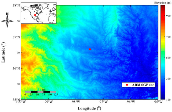
Figure 1.
SGP station of the ARM facility.
2.1.2. BLH Retrieval Using RS
RS is commonly used to determine BLH [27]. The ARM facility provides the PBL types and BLHs for RS measurements. The PBL types were computed following the method of Liu and Liang [4], whereas the BLHs were derived using the bulk Richardson (BRN) method. The PBL types can be classified into the three major regimes, namely, CBL, NBL, and SBL [1,4]. Near-surface potential temperature gradients were used to identify the boundary layer regime. The following criteria were used to identify these regimes:
where θ is potential temperature, and its subscript number denotes for the data level index assuming surface air at level = 1. θ5 and θ2 represent the fifth and second levels of the near-surface thermal, respectively. The values of on land and on ocean/ice surface were 1.0 K and 0.2 K, respectively.
BRN was used to estimate the BLH [9,28]. The BRN at height z AGL was defined as
where g denotes acceleration due to gravity, and denote the virtual potential temperatures at the surface and height z, respectively, and and denote the wind speed components at height z. The critical threshold of 0.25 was used in the BLH estimation.
2.2. Methodology
2.2.1. The Variance Method
The variance method defines turbulence as significant when a given threshold is exceeded. Previous studies show that BLH can be estimated based on a specified threshold by comparing with RS measurements. A threshold of 0.04 m2s−2 was initially set to estimate the BLH based on the TexAQS-2006 dataset [8]. BLHs from London, UK were defined at a height where > 0.1 m2s−2 [29], and this same threshold was used to estimate the BLHs in an urban environment in Beijing, China [20]. The SGP station was located near an urban environment. Therefore, a threshold of 0.1 m2s−2 was used in estimating BLH [12].
2.2.2. The Peak Method
The peak method was used to automatically detect BLH by using the DL . This method sets an automatic threshold based on the peaks for the estimation. A point in a discrete profile was defined as a peak when its value exceeds that of its neighbors. The peak method involves the following steps [24]:
Finding thresholds based on peak values. First, given an original threshold , the peak method filters the tiny scale effects, and only the data above this threshold were used to find the peaks. This method was also used to calculate the background level , which refers to the mean velocity variance on the part of the profile below . This level can be computed as
The peaks above were then detected. The thresholds based on these peaks can be calculated as
The BLH was equal to the highest point of threshold and lower than the position of threshold . In this study, the was used to filter the effect of high cloudy layers; therefore, the height of the should be higher than the BLH. BLHs are referred to the height where the is equal to 0.1 m2s−2. Therefore, = 0.05 m2s−2 was empirically set. In a profile where the values of are large or small, may be too small to filter the effect of high layer or too large to estimate the BLHs.
2.2.3. The WCT Method
The WCT method is widely used to estimate the BLHs based on data from aerosol lidar. In the WCT method, the Haar wavelet function was defined as [18]
where r is the altitude, a is the spatial extent or dilation of the function, and b is the center of the Haar function. WCT of Haar function defined as
where is the profile about , and are the lower and the higher limit of the profile, respectively. When reaches the local maximum with a coherent scale of a, value b is usually considered the PBLH.
2.2.4. The ED Method
ED is widely used in the field of image processing [30]. This method considers the gradient of a 2D change to accurately determine the abrupt edge of an image. For the time series images of DL, the BLHs were defined as the positions where a sudden change in wind speed is detected. Therefore, the image ED method provides another way of estimating BLH. The ED method involves three main steps. First, SNR and noise were used to control the quality of primary data shown in Figure 2a. Second, the edge of BLHs was detected by searching the edges of the turbulence region, which is located between the minimum and maximum peaks of . To get the minimum and maximum peaks, the number of peaks should be more than 2. The data in the turbulence region were set to 1 and others were set to 0; the binary image was shown in Figure 2b. Then, the difference between the adjacent data (back-front) was determined to obtain an edge with a value of either −1 or 1; to show a binary image of the edge, the difference result was calculated as the absolute value shown in Figure 2c. Third, the BLHs were estimated based on a theory of the diurnal cycle of PBL shown in Figure 2d. In general, the BLH is the position where the value of edge is equal to −1. However, the BL has the diurnal variation. At the daytime, the BLH was defined as the position of the weakened turbulence, to avoid the estimation of abnormal BLH, the information of the former BLH was used to limit the height of BLH. The BLH was the height with the least difference from the previous one. At nighttime, the PBL exists on two layers, the lower SBL, and the higher residual layer. Therefore, BLH was the position where the lowest value equals −1. Unfortunately, there are likely to be some abnormal BLH values in the middle, or cases where BLH cannot be calculated. When the BLH changes more than 300 m between a time resolution, it is regarded as abnormal. Therefore, the difference between BLH and the before and after values was computed. When the difference is greater than 300 m, the average value of the before and after BLH is used to replace the current BLH. In addition, this measure was used to fill the BLH that cannot be estimated.
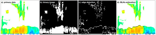
Figure 2.
BLHs estimated by the ED method.
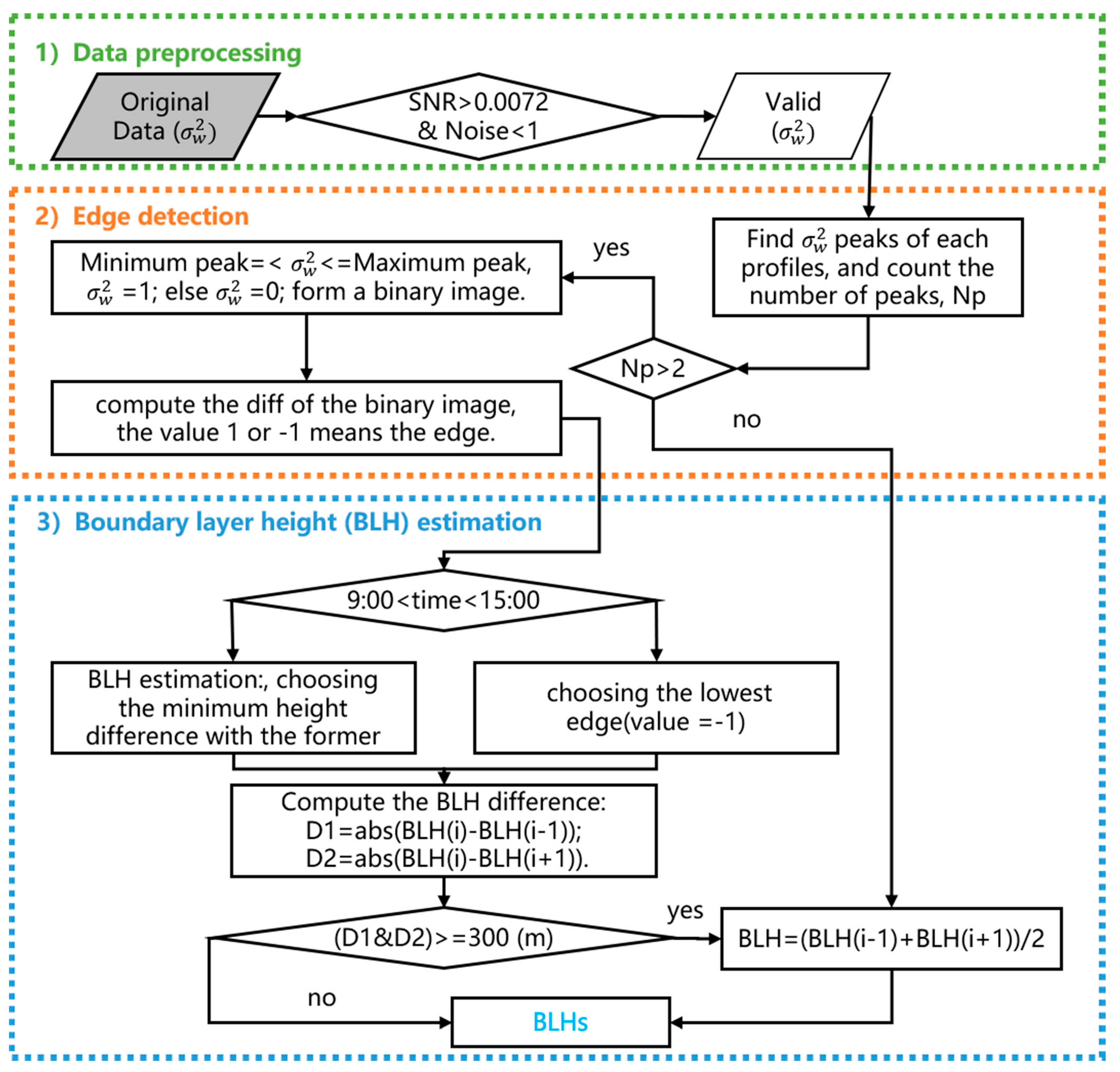
The flowchart of ED is depicted in Figure 3. The aforementioned steps are described in detail, as follows:
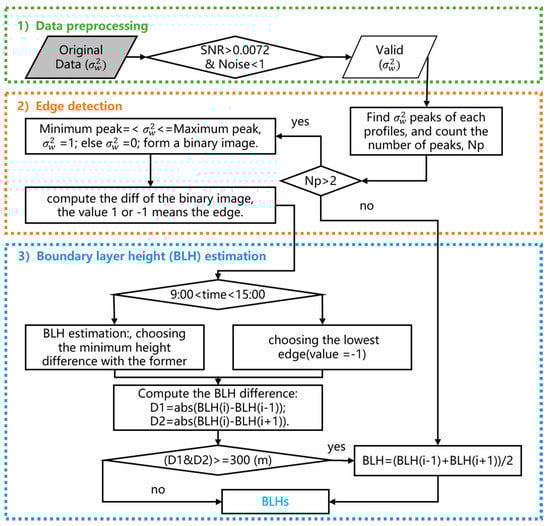
Figure 3.
Flowchart for the ED method.
Data preprocessing. To reduce the influence of data noise, controlling the quality of data is necessary. The SNR threshold (SNR = 0.0072) [21] and noise threshold (noise = 1) [19] were set to filter the noise and obtain valid data.
Edge detection. The peak value of the data obtained in step 1 was obtained, and then the number of peaks (Np) was calculated. If Np exceeds 2, then the data exceeding the minimum peak value and below the maximum peak value were set to 1, whereas the others were set to 0 to generate a binary image. The difference between the adjacent data (back-front) was determined to obtain an edge with a value of either −1 or 1. Meanwhile, if Np is less than 2, then the data cannot be estimated by BLH.
BLH estimation. Given a time processing mechanism, at daytime (9:00–15:00), the height of the edge (value = −1) with the smallest difference from the BLH for the previous period was treated as the BLH. At nighttime, a residual layer was set above the boundary layer instead of connecting a free atmosphere between these layers. Therefore, the upper edge (value = −1) of the lower layer was treated as the BLH. To eliminate the influence of a single BLH value, the differences and were calculated as
If and both exceeded 300 m, then the BLH was replaced by the average value of the former and latter BLHs. The BLH values were then outputted.
3. Results and Discussion
The from 2018 to 2020 were used to evaluate the performance of ED. The BLHs computed using the variance, peak, and ED methods were compared with the RS measurements in three ways. Including the two cases in the diurnal cycle analysis, the BLHs derived using the variance, peak, and ED methods were compared with the RS measurements under the NBL, SBL, and CBL, and a long-term analysis of the hourly and monthly BLHs for the diurnal and annual cycles was conducted. The BLHs retrieved via RS measurements from the SGP station of the ARM facility were treated as ground truths.
3.1. Analysis of Diurnal Cases
To evaluate the performance of ED, the BLHs derived using the variance, peak, and ED methods were compared with the RS measurements under extreme and routine atmospheric conditions. Two cases were considered to analyze the performance of ED.
3.1.1. Extreme Atmospheric Condition
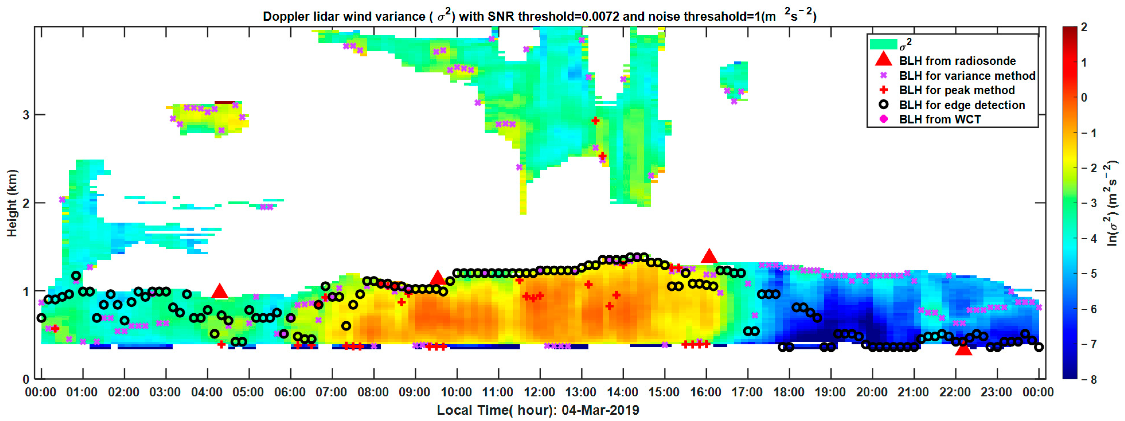
The recorded on 4 March 2019 was used to estimate the BLHs via the variance, peak, and ED methods, and the estimated BLHs were then compared with the corresponding RS measurements shown in Figure 4. The red triangle represents the BLHs obtained using RS, and the color gradient represents the DL . The purple x, red cross, and black circle represent the BLHs derived from the variance, peak, and ED methods, respectively. Most of the BLHs obtained using the variance method were overestimated and had a chaotic distribution. Meanwhile, many of the BLHs obtained using the peak method were empty, and a few BLHs were overestimated. The BLHs obtained using ED were stable and were highly consistent with the RS measurements.
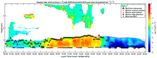
Figure 4.
BLHs on 4 March 2019 obtained using the variance, peak, and ED methods compared with the RS measurements.
The variance and peak methods were easily affected by the value of . Therefore, these methods tend to underestimate or overestimate the BLHs due to the large variances in . By contrast, ED can steadily estimate the BLHs and is not affected by the variances in , and the BLHs recorded in the diurnal cycle were consistent with the RS measurements. The variance and peak methods performed poorly probably due to extreme atmospheric conditions, and using a single threshold cannot adapt well to atmospheric variations, thereby resulting in inaccurate estimations of BLHs. By contrast, ED estimates the BLHs based on the variation in data and can avoid the influence of atmospheric conditions.
3.1.2. Routine Atmospheric Condition
The recorded on 8 July 2019 was used to estimate the BLHs via the variance, peak, and ED methods and was compared with the corresponding RS measurements shown in Figure 5. The red triangle represents the BLHs obtained using RS, and the color gradient represents the . The purple x, red cross, and black circle represent the BLHs derived from the variance, peak, and ED methods, respectively. At nighttime (00:00–06:00 and 18:00–00:00), the BLHs obtained using the variance method were higher than the RS measurements. The peak method cannot calculate the BLHs. By contrast, ED can provide stable and continuous BLH measurements with slight differences from the RS measurements.
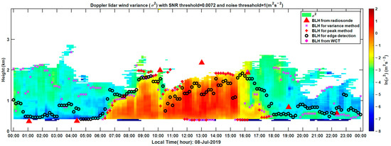
Figure 5.
BLHs on 8 July 2019 obtained using the variance, peak, and ED methods compared with the RS measurements.
The variance and peak methods performed poorly compared with ED at nighttime. The BLHs obtained using the variance and peak methods were consistent with the RS measurements from 06:00 to 12:00. But a few retrieved BLHs obtained using the variance and peak methods are higher and empty. In addition, the BLHs obtained by the variance and peak methods largely differed from the RS measurements retrieved between 12:00 and 18:00. By contrast, ED performs steadily and is highly consistent with RS measurements at daytime. The values of were much larger than the threshold, which may lead to the underestimation of BLHs on the nearest surface. The turbulence at daytime was stronger than that at nighttime. Therefore, the values of were relatively higher at daytime and were lower at nighttime. A single threshold of could not estimate the BLHs in the diurnal cycle. The peak method was unable to calculate the BLHs due to the lack of obviousness of the contour profiles. However, on the basis of the peak value of , ED extracted the atmospheric turbulence movement area to obtain the edge of BLHs and then selected the corresponding BLHs according to the diurnal change characteristics. Therefore, ED is not easily affected by the value of and returns better estimations of BLHs than the variance and peak methods.
3.2. Statistical Comparison
The BLHs obtained using the variance, peak, and ED methods were then compared with the RS measurements under NBL, SBL, and CBL. These BLHs were matched with the RS measurements for the same moment. The BLH measurements obtained using RS were selected as the middle values of the detection period. The valid samples of the peak method were selected to compute the R and RMSE between the peak and RS measurements.
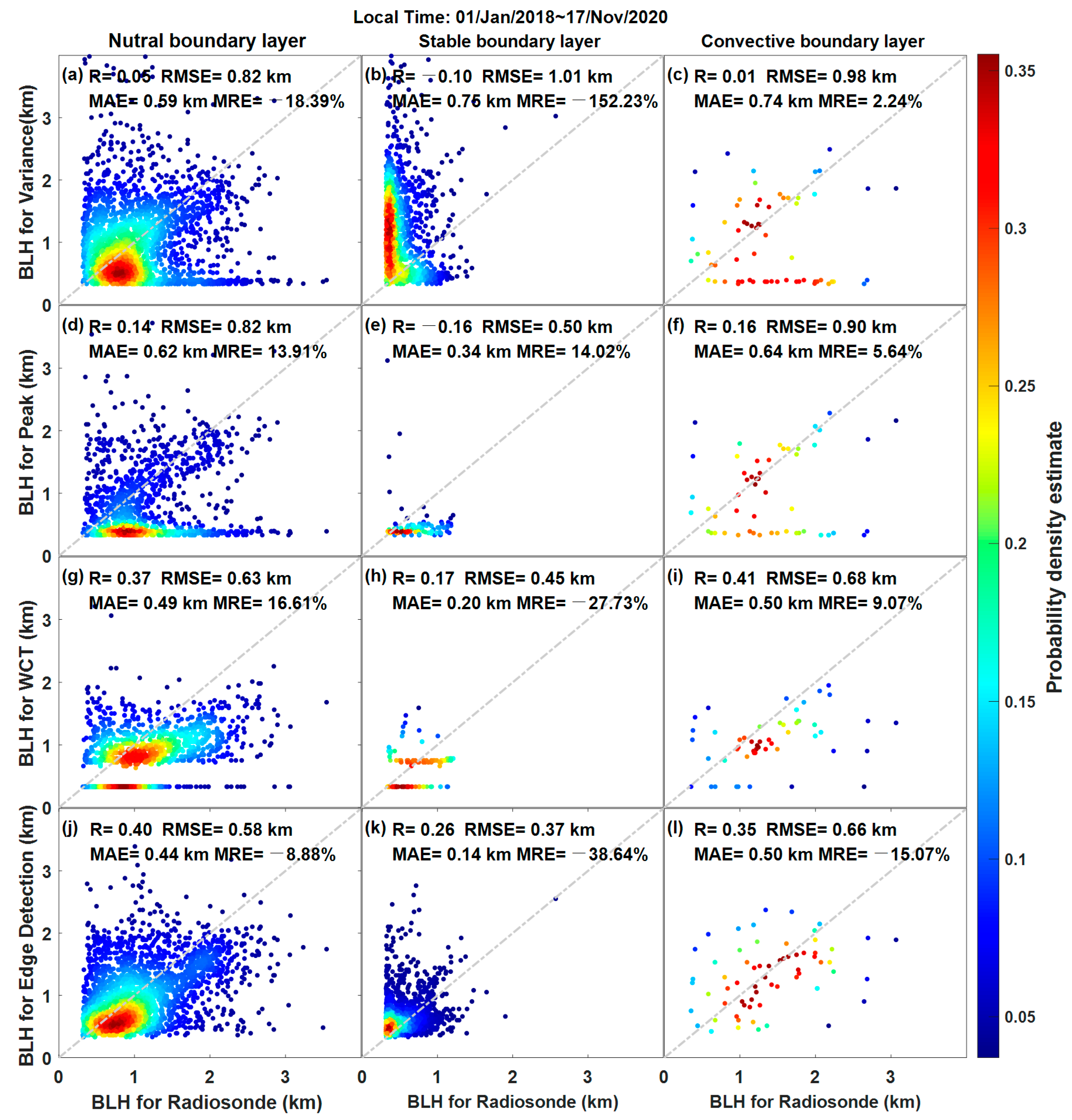
Data from 2018 to 2020 were used to verify the consistency of the three methods with RS under NBL, SBL, and CBL, respectively, as shown in Figure 6. A redder color corresponds to denser dots and more BLHs. The black dotted line represents the reference line with a slope of 1. On the NBL, SBL, and CBL, the R obtained by ED was larger than those obtained by the variance and peak methods (R: 0.4 vs. 0.05, 0.14; 0.26 vs. −0.10, −0.16; 0.35 vs. 0.01, 0.16). Meanwhile, the RMSE obtained by ED was smaller than those obtained by the variance and peak methods (RMSE: 0.58 km vs. 0.82 km, 0.82 km; 0.37 km vs. 1.01 km, 0.5 km; 0.66 km vs. 0.98 km, 0.90 km). The mean absolute error (MAE) of the ED method under the NBL, SBL, and CBL conditions are lower than the variance and peak methods (MAE: 0.44, 0.14, 0.50 vs. 0.62, 0.34, 0.64; 0.59, 0.75, 0.74), respectively. The mean relative error (MRE) of the ED method is lower than the variance and peak methods under the CBL condition (MRE: −8.88% vs. −18.39%, 13.91%). Under the SBL, the MRE of the ED method is lower than the variance method and higher than the peak method (−38.64%, vs. −152.23%; 14.02%), respectively. Under the CBL, the MRE of the ED method is lower than the variance method and higher than the peak method (−15.07% vs. 2.24%; 5.64%), respectively. In addition, more BLHs (points at which color change from deep red to shallow blue) derived from the ED method are close to the reference line than those derived from the variance and peak methods. The lower MRE of the ED method makes its result reliable. In conclusion, the result of the ED method is more consistent with the variance and peak methods under the same conditions. Although, the R of these methods were all low.
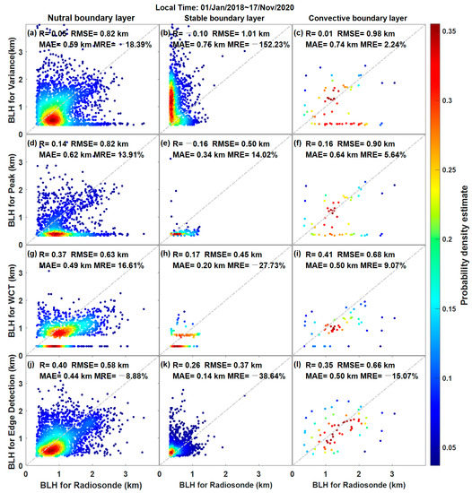
Figure 6.
BLHs from 2018 to 2020 obtained using the variance, peak, WCT, and ED methods compared with the RS measurements.
Huge differences were observed between the BLHs obtained by the variance and peak methods and the RS measurements, and most of the BLHs obtained by the traditional methods were either overestimated or underestimated. Few of the BLHs obtained using ED were either overestimated or underestimated, but the majority approached the reference line. The temporal resolution of the BLHs based on DL was 10 min, and the detection time for the RS measurements was about 30 min from launch to detection. After its launching, the balloon may change its location due to atmospheric winds. Therefore, the time and position of the retrieved BLHs and RS measurements might not match, which may explain the weak R and large RMSE. In addition, the in clear air was retrieved below the lowest cloud base, which may explain why the above methods underestimated the BLHs occasionally. Any method has its drawback. The ED method cannot estimate the BLHs when peaks of a profile are below two, which is determined by the situation of the data. Though we will use the mean substitution for adjacent data, sometimes, some errors can occur. The ED method considers the time dimension of the BLHs; it can fill the missing of uncalculated BLHs and eliminate a single abnormal BLH. The continued abnormal BLHs cannot be identified, and the missing long-term BLHs will be replaced by one value. Then, the BLHs may lose reliability. More importantly, we found that the SNR data filtered more information of (such as the white area in Figure 4 and Figure 5). Therefore, improving the SNR of the data may improve the results.
We used the WCT methods to estimate the BLHs for the DL dataset from 2018 to 2020 and compared those results with the RS measurements under the NBL, SBL, and CBL conditions, as shown in Figure 6g–i. The R between the ED method and RS measurements are larger than the WCT method under the NBL and SBL conditions and smaller under the CBL condition (R: 0.4, 0.26, 0.35 vs. 0.37, 0.17, 0.41). The RMSE and MAE between the ED method and RS measurements are larger than those in the WCT method under the NBL, SBL, and CBL conditions, (RMSE (km): 0.58, 0.37, 0.66 vs. 0.63, 0.45, 0.68; MAE: 0.44, 0.14, 0.50 vs. 0.49, 0.20, 0.50). The MRE between the ED method and RS measurements are larger than that in the WCT method under the NBL condition and smaller under the SBL and CBL conditions (MRE: −8.88%, −38.64%, −15.07% vs. 16.61%, −27.73%, 9.07%). Due to the in clear air that are captured below the lowest cloud base, the clouds’ effect was eliminated. The results of the ED method and the WCT method are similar, and the performance of the ED method is even better, combined with the analysis of the above factors. In addition, many BLHs derived from the WCT method were significantly underestimated under the NBL condition and overestimated under the SBL condition.
Compared with those methods proposed to estimate the BLHs based on the aerosol lidar, the ED method has a poor performance. Dang, Yang [31] improved the WCT method with a given top limiter altitude to reduce the interference of RL and cloud layer on BLHs estimation. The method was well performed and showed good results (R = 0.79) validated by radiosonde. Li, Chang [32] proposed the combining of the whale optimization algorithm and the top limit method to estimate the BLHs based on micro-pulse lidar. The R between this method, WCT, and gradient methods and RS measurements are 0.88, 0.82, and 0.78, respectively. Sleeman, Halem [33] proposed a deep learning method by employing deep neural networks for denoising and image segmentation to estimate the BLH, and it can infer BLHs in the presence of dense clouds. The results for this method are similar to the WCT method compared with the RS measurements. Among these methods, the WCT method was selected as the reference to estimated BLH from DL. Unfortunately, the results retrieved from the WCT method are not very well in this study, possibly because of the lower SNR and vertical resolution of the DL data. It is necessary to improve the quality of the DL signal for accurate BLHs. Comparatively speaking, the ED method also has better performance with the WCT method under the NBL, SBL, and CBL conditions. The poor performance of the ED method motivates us to improve or/and develop more practical approaches.
3.3. Long-Term Analysis
In this section, the BLHs from 2018 to 2020 derived using the variance, peak, and ED methods were used to analyze the long-term variations in the BLHs. Therefore, hourly average BLHs were used for the diurnal analysis, and monthly average BLHs were used for the annual analysis. The DL data for November and December 2020 were limited.
3.3.1. Diurnal Cycle
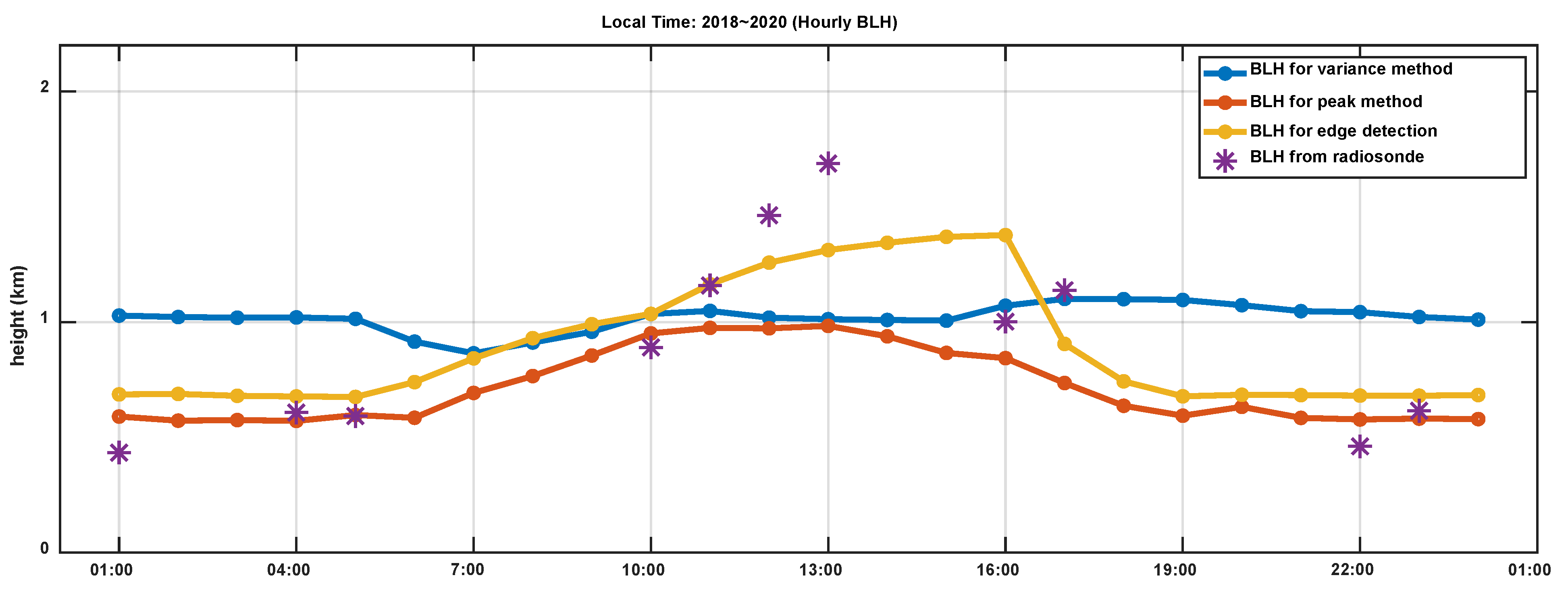
The hourly average BLHs are shown in Figure 7. The blue, orange, and yellow point lines represent the mean BLHs per hour in 2019 retrieved using the variance, peak, and ED methods, respectively. The purple asterisk represents the RS measurements for each hourly BLH.
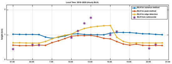
Figure 7.
Hourly BLHs retrieved using the variance, peak, and ED methods.
The hourly BLHs retrieved using the variance method were higher and lower than those obtained by RS measurements at nighttime (from 00:00 to 06:00 and from 18:00 to 24:00). BLHs obtained using the variance method were higher than RS measurements at 12:00. The BLHs remained stable from 07:00 to 14:00 and increased from 14:00 to 17:00. The BLHs obtained using the peak method slowly increased from 06:00 to 12:00 and decreased from 12:00 to 18:00. The BLHs retrieved using ED increased from 06:00 to 16:00, decreased from 16:00 to 18:00, and remained stable from 18:00 to 24:00. The difference between the peak and ED methods and RS measurements are both small.
The BLHs generally increased at sunrise and decreased at sunset. Therefore, the daytime BLHs should be higher than the nighttime BLHs. In the long-term analysis for the diurnal cycle, the BLHs retrieved by ED were more consistent with theory compared with those retrieved using the variance and peak methods. Moreover, the standard error of the ED method was smaller than those of the variance and peak methods, thereby suggesting that the BLHs retrieved by ED were close to the mean values.
3.3.2. Annual Cycle
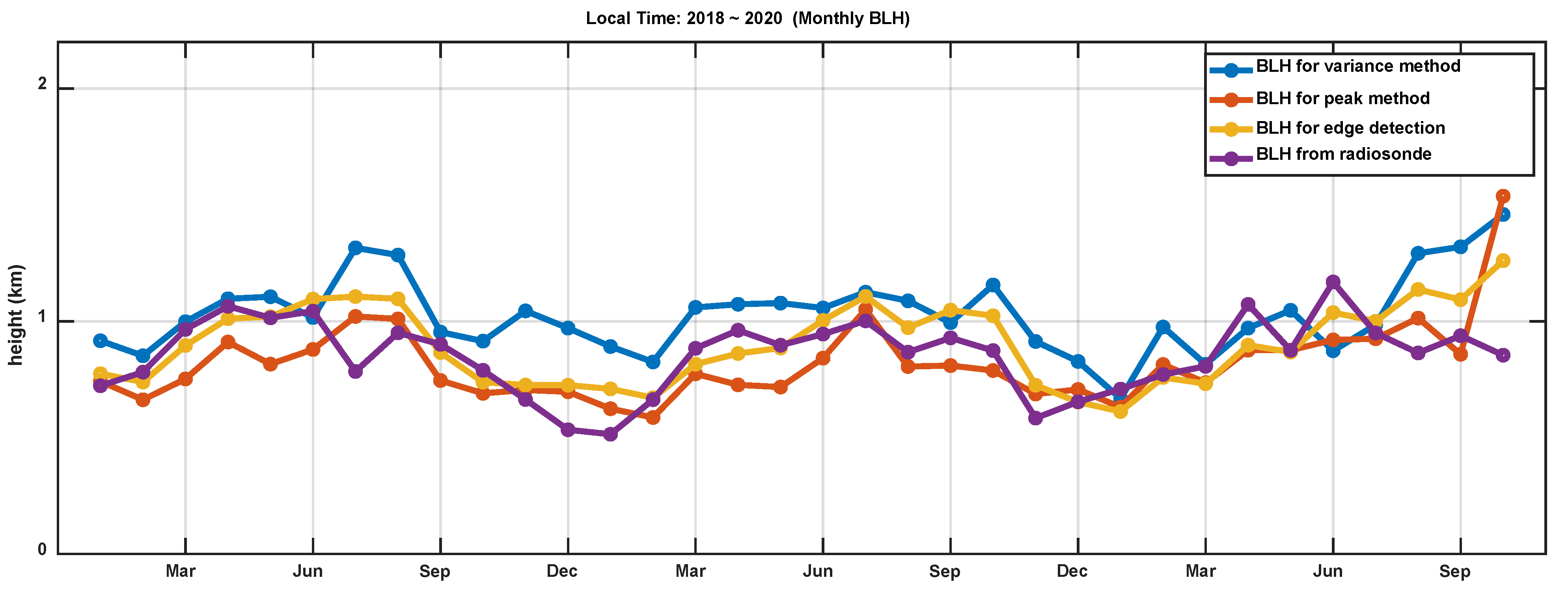
The monthly average BLHs derived using the variance, peak, and ED methods and the RS measurements are shown in Figure 8. The blue, orange, yellow, and purple point lines represent the monthly mean BLHs from 2018 to 2020, retrieved using the variance, peak, and ED methods and RS measurements in the annual cycle, respectively. The monthly BLHs for the variances greatly differed from the RS measurements, particularly from June 2018 to June 2019. The monthly BLHs retrieved using the ED and peak methods were consistent with the RS measurements. However, there are differences between April and May 2018, and 2019. The monthly BLHs for November and December 2020 were limited. The BLHs from 2018 to 2020 retrieved using ED showed consistent trends with the RS measurements, although there is a big difference for these monthly BLHs in October 2020. The annual cycle BLHs showed that the BLHs in summer and autumn were higher than those in spring and winter. The BLHs increased slowly from January to May and stably decreased from June to December.
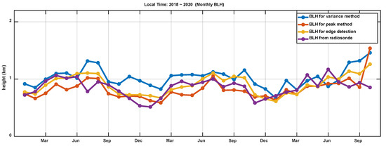
Figure 8.
Monthly BLHs retrieved using the variance, peak, and ED methods and the RS measurements.
4. Conclusions
This paper introduced ED for estimating BLHs based on DL . The two cases on 4 March 2019 and 8 July 2019 were used to estimate the BLHs via the variance, peak, and ED methods in the diurnal cycle. The retrieved BLHs were compared with the RS measurements, and the results show that ED was more accurate than the variance and peak methods under extreme and routine atmospheric conditions. Therefore, ED can estimate the BLHs in the diurnal cycle and perform better than the other two methods. The BLHs retrieved using the variance, peak, WCT, and ED methods from 2018 to 2020 were compared with the RS measurements under NBL, SBL, and CBL. The results show that ED was more consistent and had lower RMSE with the RS measurements than the variance and peak methods under NBL, SBL, and CBL. The lower MAE and MRE indicated the results of the ED method with reliability, and a number of the BLHs derived from the ED method are closer to the reference line than those obtained by the variance and peak methods. In addition, the ED method has similar results with the WCT method and is even better. In the long-term analysis, the hourly BLHs retrieved by ED were consistent with theory, whereas those retrieved using the variance and peak methods were not. The monthly BLHs retrieved using the peak and ED methods were more consistent with the RS measurements than those obtained using the variance method. The BLHs recorded in summer and autumn were also higher than those in spring and winter.
In general, the ED method can estimate the BLHs in the diurnal cycle under extreme and routine atmospheric conditions and has a better performance than the variance, peak, and WCT methods. But the performance of these methods are unsatisfactory at present. Direct detection of turbulence changes can obtain accurate BLH theoretically, but the low SNR of DL may be one of the reasons that reduces the accuracy of the BLHs obtained from this remote sensing equipment. The poor performance of the ED method motivates us to improve or/and develop more practical approaches moving forward.
Author Contributions
Conceptualization, Y.P. and W.W.; Funding acquisition, W.W.; Investigation, Y.P. and Z.J.; Methodology, Y.P., Z.J. and W.W.; Software, Y.P. and Z.J.; Supervision, W.W.; Validation, Y.P., Z.J. and W.W.; Visualization, Y.P., Z.J., P.T., W.X. and W.W.; Writing—original draft, Y.P. and W.W.; Writing—review and editing, W.W. All authors have read and agreed to the published version of the manuscript.
Funding
This study was supported by the National Natural Science Foundation of China (41901295); the Natural Science Foundation of Hunan Province, China (2020JJ5708).
Institutional Review Board Statement
Not applicable.
Informed Consent Statement
Not applicable.
Data Availability Statement
Data supporting reported results can be found on the data discovery of ARM facility (https://adc.arm.gov/discovery). Data accessed on 20 April 2021.
Acknowledgments
We are grateful for the data discovery service of ARM (https://adc.arm.gov/discovery, accessed on 1 July 2021).
Conflicts of Interest
The authors declare no conflict of interest.
References
- Stull, R.B. An Introduction to Boundary Layer Meteorology; Springer: Berlin, Germany, 1988. [Google Scholar]
- Garratt, J. Review: The atmospheric boundary layer. Earth-Sci. Rev. 1994, 37, 89–134. [Google Scholar] [CrossRef]
- Manninen, A.J.; Marke, T.; Tuononen, M.; O’Connor, E.J. Atmospheric Boundary Layer Classification with Doppler Lidar. J. Geophys. Res. Atmos. 2018, 123, 8172–8189. [Google Scholar] [CrossRef]
- Liu, S.; Liang, X.Z. Observed Diurnal Cycle Climatology of Planetary Boundary Layer Height. J. Clim. 2010, 23, 5790–5809. [Google Scholar] [CrossRef]
- Dang, R.; Yang, Y.; Hu, X.-M.; Wang, Z.; Zhang, S. A Review of Techniques for Diagnosing the Atmospheric Boundary Layer Height (ABLH) Using Aerosol Lidar Data. Remote Sens. 2019, 11, 1590. [Google Scholar] [CrossRef] [Green Version]
- Steyn, D.G.; Baldi, M.; Hoff, R.M. The Detection of Mixed Layer Depth and Entrainment Zone Thickness from Lidar Backscatter Profiles. J. Atmos. Ocean. Technol. 1999, 16, 953–959. [Google Scholar] [CrossRef]
- Brooks, I.M. Finding Boundary Layer Top: Application of a Wavelet Covariance Transform to Lidar Backscatter Profiles. J. Atmos. Ocean. Technol. 2003, 20, 1092–1105. [Google Scholar] [CrossRef] [Green Version]
- Tucker, S.C.; Senff, C.J.; Weickmann, A.M.; Brewer, W.A.; Banta, R.; Sandberg, S.P.; Law, D.C.; Hardesty, R.M. Doppler Lidar Estimation of Mixing Height Using Turbulence, Shear, and Aerosol Profiles. J. Atmos. Ocean. Technol. 2009, 26, 673–688. [Google Scholar] [CrossRef]
- Seibert, P. Review and intercomparison of operational methods for the determination of the mixing height. Atmos. Environ. 2000, 34, 1001–1027. [Google Scholar] [CrossRef]
- Wang, F.; Yang, T.; Wang, Z.; Chen, X.; Wang, H.; Guo, J. A comprehensive evaluation of planetary boundary layer height retrieval techniques using lidar data under different pollution scenarios. Atmos. Res. 2021, 253, 105483. [Google Scholar] [CrossRef]
- Miao, Y.; Liu, S.; Guo, J.; Huang, S.; Yan, Y.; Lou, M. Unraveling the relationships between boundary layer height and PM2.5 pollution in China based on four-year radiosonde measurements. Environ. Pollut. 2018, 243, 1186–1195. [Google Scholar] [CrossRef] [PubMed]
- Lloyd, M.R. Doppler LiDAR Measurements of Boundary Layer Heights over San Jose, California. Ph.D. Thesis, San Jose State University, San Jose, CA, USA, 2019. [Google Scholar]
- Frehlich, R.; Meillier, Y.; Jensen, M.L.; Balsley, B.; Sharman, R. Measurements of Boundary Layer Profiles in an Urban Environment. J. Appl. Meteorol. Clim. 2006, 45, 821–837. [Google Scholar] [CrossRef]
- Newsom, R.K.; Krishnamurthy, R. Doppler Lidar (DL) Instrument Handbook; DOE Office of Science Atmospheric Radiation Measurement (ARM) User Facility: Lemont, IL, USA, 2020. [Google Scholar]
- Strawbridge, K.; Snyder, B. Planetary boundary layer height determination during Pacific 2001 using the advantage of a scanning lidar instrument. Atmospheric Environ. 2004, 38, 5861–5871. [Google Scholar] [CrossRef]
- Menut, L.; Flamant, C.; Pelon, J.; Flamant, P.H. Urban boundary-layer height determination from lidar measurements over the Paris area. Appl. Opt. 1999, 38, 945–954. [Google Scholar] [CrossRef] [PubMed]
- Fan, S.; Gao, Z.; Kalogiros, J.; Li, Y.; Yin, J.; Li, X. Estimate of boundary-layer depth in Nanjing city using aerosol lidar data during 2016–2017 winter. Atmos. Environ. 2019, 205, 67–77. [Google Scholar] [CrossRef]
- Compton, J.C.; Delgado, R.; Berkoff, T.A.; Hoff, R.M. Determination of Planetary Boundary Layer Height on Short Spatial and Temporal Scales: A Demonstration of the Covariance Wavelet Transform in Ground-Based Wind Profiler and Lidar Measurements*. J. Atmos. Ocean. Technol. 2013, 30, 1566–1575. [Google Scholar] [CrossRef]
- Newsom, R.K.; Sivaraman, C.; Shippert, T.R.; Riihimaki, L.D. Doppler Lidar Vertical Velocity Statistics Value-Added Product; DOE ARM Climate Research Facility: Washington, DC, USA, 2015. [Google Scholar]
- Huang, M.; Gao, Z.; Miao, S.; Chen, F.; LeMone, M.A.; Li, J.; Hu, F.; Wang, L. Estimate of Boundary-Layer Depth over Beijing, China, Using Doppler Lidar Data During SURF-2015. Bound.-Layer Meteorol. 2017, 162, 503–522. [Google Scholar] [CrossRef] [Green Version]
- Berg, L.K.; Newsom, R.K.; Turner, D. Year-Long Vertical Velocity Statistics Derived from Doppler Lidar Data for the Continental Convective Boundary Layer. J. Appl. Meteorol. Clim. 2017, 56, 2441–2454. [Google Scholar] [CrossRef]
- Villalonga, J.; Beveridge, S.L.; Da Silva, M.P.A.; Tanamachi, R.L.; Rocadenbosch, F.; Turner, D.D.; Frasier, S.J. Convective boundary-layer height estimation from combined radar and Doppler lidar observations in VORTEX-SE. Remote Sens. Clouds Atmos. 2020, 11531, 115310X. [Google Scholar]
- Drew, D.R.; Barlow, J.F.; Lane, S.E. Observations of wind speed profiles over Greater London, UK, using a Doppler lidar. J. Wind. Eng. Ind. Aerodyn. 2013, 121, 98–105. [Google Scholar] [CrossRef] [Green Version]
- Automatic Detection of Boundary Layer Height Using Doppler Lidar Measurements. Available online: https://hal.archives-ouvertes.fr/meteo-01379589/ (accessed on 26 August 2021).
- Xiang, Y.; Ye, Q.; Liu, J.; Zhang, T.; Fan, G.; Zhou, P.; Lü, L.; Liu, Y. Retrieve of planetary boundary layer height based on image edge detection. Chin. J. Lasers 2016, 43, 0704003. [Google Scholar] [CrossRef]
- Li, H.; Yang, Y.; Hu, X.-M.; Huang, Z.; Wang, G.; Zhang, B.; Zhang, T. Evaluation of retrieval methods of daytime convective boundary layer height based on lidar data. J. Geophys. Res. Atmos. 2017, 122, 4578–4593. [Google Scholar] [CrossRef]
- Sivaraman, C.; McFarlane, S.; Chapman, E.; Jensen, M.; Toto, T.; Liu, S.; Fischer, M. Planetary Boundary Layer (PBL) Height Value Added Product (VAP): Radiosonde Retrievals; US Department of Energy: Washington, DC, USA, 2013. [Google Scholar]
- Sørensen, J.H.; Rasmussen, A.; Ellermann, T.; Lyck, E. Mesoscale influence on long-range transport—evidence from ETEX modelling and observations. Atmos. Environ. 1998, 32, 4207–4217. [Google Scholar] [CrossRef]
- Barlow, J.F.; Dunbar, T.M.; Nemitz, E.G.; Wood, C.R.; Gallagher, M.W.; Davies, F.; O’Connor, E.; Harrison, R.M. Boundary layer dynamics over London, UK, as observed using Doppler lidar during REPARTEE-II. Atmos. Chem. Phys. Discuss. 2011, 11, 2111–2125. [Google Scholar] [CrossRef] [Green Version]
- Versaci, M.; Morabito, F.C. Image Edge Detection: A New Approach Based on Fuzzy Entropy and Fuzzy Divergence. Int. J. Fuzzy Syst. 2021. [Google Scholar] [CrossRef]
- Dang, R.; Yang, Y.; Li, H.; Hu, X.-M.; Wang, Z.; Huang, Z.; Zhou, T.; Zhang, T. Atmosphere Boundary Layer Height (ABLH) Determination under Multiple-Layer Conditions Using Micro-Pulse Lidar. Remote Sens. 2019, 11, 263. [Google Scholar] [CrossRef] [Green Version]
- Li, H.; Chang, J.; Liu, Z.; Zhang, L.; Dai, T.; Chen, S. An improved method for automatic determination of the planetary boundary layer height based on lidar data. J. Quant. Spectrosc. Radiat. Transf. 2020, 257, 107382. [Google Scholar] [CrossRef]
- Sleeman, J.; Halem, M.; Yang, Z.; Caicedo, V.; Demoz, B.; Delgado, R. A deep machine learning approach for lidar based boundary layer height detection. In Proceedings of the IGARSS 2020–2020 IEEE International Geoscience and Remote Sensing Symposium, Online, 26 September–2 October 2020. [Google Scholar]


Publisher’s Note: MDPI stays neutral with regard to jurisdictional claims in published maps and institutional affiliations. |
© 2021 by the authors. Licensee MDPI, Basel, Switzerland. This article is an open access article distributed under the terms and conditions of the Creative Commons Attribution (CC BY) license (https://creativecommons.org/licenses/by/4.0/).