
WRF-Chem Modeling of Summertime Air Pollution in the Northern Great Plains: Chemistry and Aerosol Mechanism Intercomparison

Abstract
:1. Introduction
2. Methods
2.1. Model Configuration
2.2. Model Scenario
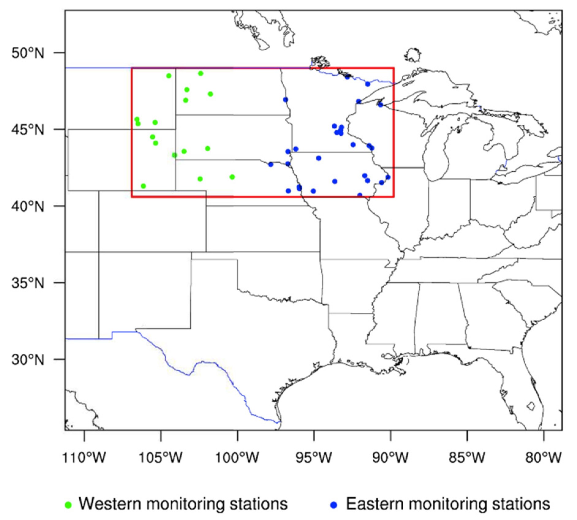
2.3. Observational Data and Analysis
3. Results and Discussion
3.1. Meteorology
3.2. Ozone
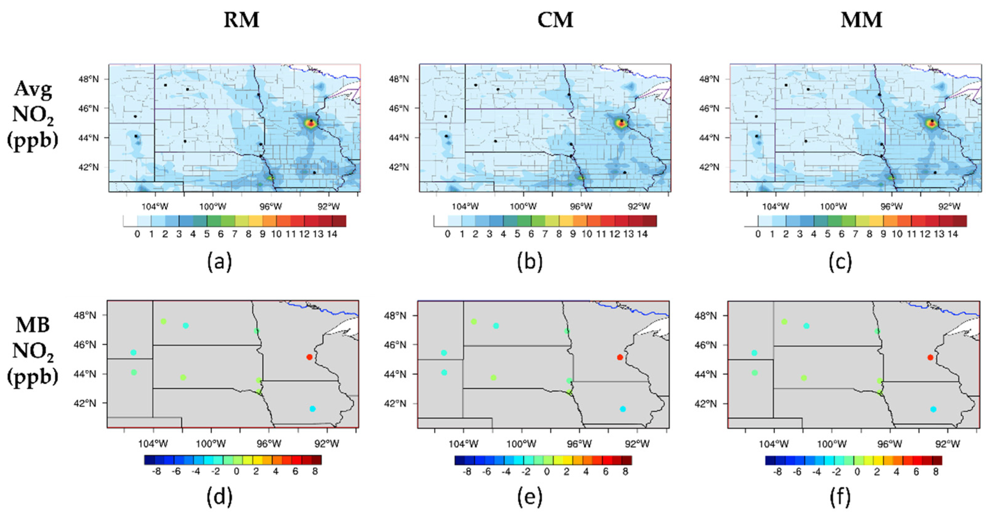
3.3. NO2
3.4. PM2.5
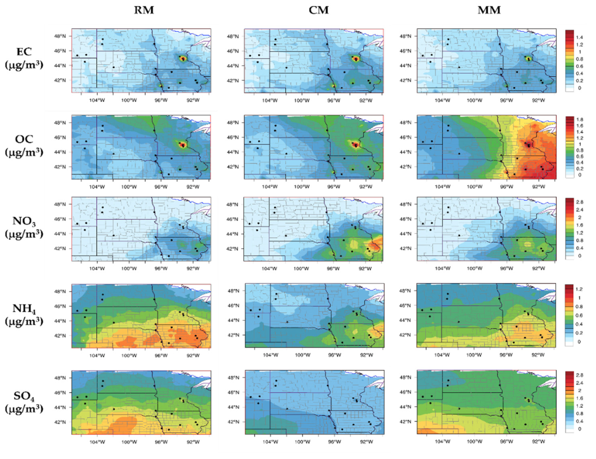
3.5. PM2.5 Subspecies
4. Conclusions
Supplementary Materials
Author Contributions
Funding
Institutional Review Board Statement
Informed Consent Statement
Data Availability Statement
Acknowledgments
Conflicts of Interest
References
- Allen, D.T. Emissions from oil and gas operations in the United States and their air quality implications. J. Air Waste Manag. Assoc. 2016, 66, 549–575. [Google Scholar] [CrossRef] [Green Version]
- Evanoski-Cole, A.R.; Gebhart, K.A.; Sive, B.C.; Zhou, Y.; Capps, S.L.; Day, D.E.; Prenni, A.J.; Schurman, M.I.; Sullivan, A.P.; Li, Y.; et al. Composition and sources of winter haze in the Bakken oil and gas extraction region. Atmos. Environ. 2017, 156, 77–87. [Google Scholar] [CrossRef]
- Homepage—U.S. Energy Information Administration (EIA). Available online: https://www.eia.gov/index.php (accessed on 2 July 2021).
- Li, C.; Hsu, N.C.; Sayer, A.M.; Krotkov, N.A.; Fu, J.S.; Lamsal, L.N.; Lee, J.; Tsay, S.-C. Satellite observation of pollutant emissions from gas flaring activities near the Arctic. Atmos. Environ. 2016, 133, 1–11. [Google Scholar] [CrossRef]
- Majid, A.; Martin, M.V.; Lamsal, L.N.; Duncan, B.N. A decade of changes in nitrogen oxides over regions of oil and natural gas activity in the United States. Elementa-Sci. Anthrop. 2017, 5, 76. [Google Scholar] [CrossRef]
- Prenni, A.J.; Day, D.E.; Evanoski-Cole, A.R.; Sive, B.C.; Hecobian, A.; Zhou, Y.; Gebhart, K.A.; Hand, J.L.; Sullivan, A.P.; Li, Y.; et al. Oil and gas impacts on air quality in federal lands in the Bakken region: An overview of the Bakken Air Quality Study and first results. Atmos. Chem. Phys. 2016, 16, 1401–1416. [Google Scholar] [CrossRef] [Green Version]
- Schwarz, J.P.; Holloway, J.S.; Katich, J.M.; McKeen, S.; Kort, E.A.; Smith, M.L.; Ryerson, T.B.; Sweeney, C.; Peischl, J. Black Carbon Emissions from the Bakken Oil and Gas Development Region. Environ. Sci. Technol. Lett. 2015, 2, 281–285. [Google Scholar] [CrossRef]
- Thompson, T.M.; Shepherd, D.; Stacy, A.; Barna, M.G.; Schichtel, B.A. Modeling to Evaluate Contribution of Oil and Gas Emissions to Air Pollution. J. Air Waste Manag. Assoc. 2017, 67, 445–461. [Google Scholar] [CrossRef] [PubMed] [Green Version]
- Nopmongcol, U.; Alvarez, Y.; Jung, J.; Grant, J.; Kumar, N.; Yarwood, G. Source contributions to United States ozone and particulate matter over five decades from 1970 to 2020. Atmos. Environ. 2017, 167, 116–128. [Google Scholar] [CrossRef]
- Yahya, K.; Wang, K.; Campbell, P.; Chen, Y.; Glotfelty, T.; He, J.; Pirhalla, M.; Zhang, Y. Decadal application of WRF/Chem for regional air quality and climate modeling over the US under the representative concentration pathways scenarios. Part 1: Model evaluation and impact of downscaling. Atmos. Environ. 2017, 152, 562–583. [Google Scholar] [CrossRef] [Green Version]
- Tessum, C.W.; Hill, J.D.; Marshall, J.D. Twelve-month, 12 km resolution North American WRF-Chem v3.4 air quality simulation: Performance evaluation. Geosci. Model. Dev. 2015, 8, 957–973. [Google Scholar] [CrossRef] [Green Version]
- Yahya, K.; Campbell, P.; Zhang, Y. Decadal application of WRF/chem for regional air quality and climate modeling over the US under the representative concentration pathways scenarios. Part 2: Current vs. future simulations. Atmos. Environ. 2017, 152, 584–604. [Google Scholar] [CrossRef] [Green Version]
- Abdallah, C.; Sartelet, K.; Afif, C. Influence of boundary conditions and anthropogenic emission inventories on simulated O3 and PM2.5 concentrations over Lebanon. Atmos. Pollut. Res. 2016, 7, 971–979. [Google Scholar] [CrossRef] [Green Version]
- Werner, M.; Kryza, M.; Geels, C.; Ellermann, T.; Ambelas Skjøth, C. Ammonia Concentrations Over Europe—Application of the WRF-Chem Model Supported with Dynamic Emission. Pol. J. Environ. Stud. 2017, 26, 1323–1341. [Google Scholar] [CrossRef]
- Im, U.; Christensen, J.H.; Geels, C.; Hansen, K.M.; Brandt, J.; Solazzo, E.; Alyuz, U.; Balzarini, A.; Baro, R.; Bellasio, R.; et al. Influence of anthropogenic emissions and boundary conditions on multi-model simulations of major air pollutants over Europe and North America in the framework of AQMEII3. Atmos. Chem. Phys. 2018, 18, 8929–8952. [Google Scholar] [CrossRef] [PubMed] [Green Version]
- Gupta, M.; Mohan, M. Validation of WRF/Chem model and sensitivity of chemical mechanisms to ozone simulation over megacity Delhi. Atmos. Environ. 2015, 122, 220–229. [Google Scholar] [CrossRef]
- Balzarini, A.; Pirovano, G.; Honzak, L.; Zabkar, R.; Curci, G.; Forkel, R.; Hirtl, M.; San Jose, R.; Tuccella, P.; Grell, G.A. WRF-Chem model sensitivity to chemical mechanisms choice in reconstructing aerosol optical properties. Atmos. Environ. 2015, 115, 604–619. [Google Scholar] [CrossRef]
- Im, U.; Bianconi, R.; Solazzo, E.; Kioutsioukis, I.; Badia, A.; Balzarini, A.; Baro, R.; Bellasio, R.; Brunner, D.; Chemel, C.; et al. Evaluation of operational on-line-coupled regional air quality models over Europe and North America in the context of AQMEII phase 2. Part I: Ozone. Atmos. Environ. 2015, 115, 404–420. [Google Scholar] [CrossRef] [Green Version]
- Mar, K.A.; Ojha, N.; Pozzer, A.; Butler, T.M. Ozone air quality simulations with WRF-Chem (v3.5.1) over Europe: Model evaluation and chemical mechanism comparison. Geosci. Model. Dev. 2016, 9, 3699–3728. [Google Scholar] [CrossRef] [Green Version]
- Georgiou, G.K.; Christoudias, T.; Proestos, Y.; Kushta, J.; Hadjinicolaou, P.; Lelieveld, J. Air quality modelling in the summer over the eastern Mediterranean using WRF-Chem: Chemistry and aerosol mechanism intercomparison. Atmos. Chem. Phys. 2018, 18, 1555–1571. [Google Scholar] [CrossRef] [Green Version]
- Appel, K.W.; Napelenok, S.L.; Foley, K.M.; Pye, H.O.T.; Hogrefe, C.; Luecken, D.J.; Bash, J.O.; Roselle, S.J.; Pleim, J.E.; Foroutan, H.; et al. Description and evaluation of the Community Multiscale Air Quality (CMAQ) modeling system version 5.1. Geosci. Model. Dev. 2017, 10, 1703–1732. [Google Scholar] [CrossRef] [Green Version]
- Grell, G.A.; Peckham, S.E.; Schmitz, R.; McKeen, S.A.; Frost, G.; Skamarock, W.C.; Eder, B. Fully coupled “online” chemistry within the WRF model. Atmos. Environ. 2005, 39, 6957–6975. [Google Scholar] [CrossRef]
- Ramboll Environment and Health. User’s Guide Comprehensive Air Quality Model with Extensions Version 7.10; CAMx: Anaheim, CA, USA, 2020. [Google Scholar]
- Long, M.S.; Yantosca, R.; Nielsen, J.E.; Keller, C.A.; da Silva, A.; Sulprizio, M.P.; Pawson, S.; Jacob, D.J. Development of a grid-independent GEOS-Chem chemical transport model (v9-02) as an atmospheric chemistry module for Earth system models. Geosci. Model. Dev. 2015, 8, 595–602. [Google Scholar] [CrossRef] [Green Version]
- Mailler, S.; Menut, L.; Khvorostyanov, D.; Valari, M.; Couvidat, F.; Siour, G.; Turquety, S.; Briant, R.; Tuccella, P.; Bessagnet, B.; et al. CHIMERE-2017: From urban to hemispheric chemistry-transport modeling. Geosci. Model. Dev. 2017, 10, 2397–2423. [Google Scholar] [CrossRef] [Green Version]
- Zaveri, R.A.; Peters, L.K. A new lumped structure photochemical mechanism for large-scale applications. J. Geophys. Res. Atmos. 1999, 104, 30387–30415. [Google Scholar] [CrossRef]
- Gery, M.W.; Whitten, G.Z.; Killus, J.P.; Dodge, M.C. A photochemical kinetics mechanism for urban and regional scale computer modeling. J. Geophys. Res. Atmos. 1989, 94, 12925–12956. [Google Scholar] [CrossRef]
- Stockwell, W.R.; Middleton, P.; Chang, J.S.; Tang, X. The second generation regional acid deposition model chemical mechanism for regional air quality modeling. J. Geophys. Res. Atmos. 1990, 95, 16343–16367. [Google Scholar] [CrossRef]
- Stockwell, W.R.; Kirchner, F.; Kuhn, M.; Seefeld, S. A new mechanism for regional atmospheric chemistry modeling. J. Geophys. Res. Atmos. 1997, 102, 25847–25879. [Google Scholar] [CrossRef] [Green Version]
- Carter, W.P.L. Documentation of the SAPRC-99 Chemical Mechanism for VOC Reactivity Assessment; California Air Resources Board, Research Division: Sacramento, CA, USA, 2000. [Google Scholar]
- Emmons, L.K.; Walters, S.; Hess, P.G.; Lamarque, J.-F.; Pfister, G.G.; Fillmore, D.; Granier, C.; Guenther, A.; Kinnison, D.; Laepple, T.; et al. Description and evaluation of the Model for Ozone and Related chemical Tracers, version 4 (MOZART-4). Geosci. Model. Dev. 2010, 3, 43–67. [Google Scholar] [CrossRef] [Green Version]
- Zaveri, R.A.; Easter, R.C.; Fast, J.D.; Peters, L.K. Model for Simulating Aerosol Interactions and Chemistry (MOSAIC). J. Geophys. Res. Atmos. 2008, 113, D13204. [Google Scholar] [CrossRef]
- Ackermann, I.J.; Hass, H.; Memmesheimer, M.; Ebel, A.; Binkowski, F.S.; Shankar, U. Modal aerosol dynamics model for Europe: Development and first applications. Atmos. Environ. 1998, 32, 2981–2999. [Google Scholar] [CrossRef]
- Schell, B.; Ackermann, I.J.; Hass, H.; Binkowski, F.S.; Ebel, A. Modeling the formation of secondary organic aerosol within a comprehensive air quality model system. J. Geophys. Res. Atmos. 2001, 106, 28275–28293. [Google Scholar] [CrossRef]
- Ahmadov, R.; McKeen, S.A.; Robinson, A.L.; Bahreini, R.; Middlebrook, A.M.; de Gouw, J.A.; Meagher, J.; Hsie, E.-Y.; Edgerton, E.; Shaw, S.; et al. A volatility basis set model for summertime secondary organic aerosols over the eastern United States in 2006. J. Geophys. Res. Atmos. 2012, 117, D06301. [Google Scholar] [CrossRef]
- Sartelet, K.N.; Hayami, H.; Albriet, B.; Sportisse, B. Development and preliminary validation of a modal aerosol model for tropospheric chemistry: MAM. Aerosol Sci. Technol. 2006, 40, 118–127. [Google Scholar] [CrossRef]
- Chin, M.; Rood, R.B.; Lin, S.J.; Muller, J.F.; Thompson, A.M. Atmospheric sulfur cycle simulated in the global model GOCART: Model description and global properties. J. Geophys. Res. Atmos. 2000, 105, 24671–24687. [Google Scholar] [CrossRef]
- Do, T.N.N.; Ngo, X.T.; Pham, V.H.; Vuong, N.L.; Le, H.A.; Pham, C.T.; Bui, Q.H.; Nguyen, T.N.T. Application of WRF-Chem to simulate air quality over Northern Vietnam. Environ. Sci. Pollut. Res. 2021, 28, 12067–12081. [Google Scholar] [CrossRef] [PubMed]
- Kushta, J.; Georgiou, G.K.; Proestos, Y.; Christoudias, T.; Lelieveld, J. Modelling study of the atmospheric composition over Cyprus. Atmos. Pollut. Res. 2018, 9, 257–269. [Google Scholar] [CrossRef]
- Spiridonov, V.; Jakimovski, B.; Spiridonova, I.; Pereira, G. Development of air quality forecasting system in Macedonia, based on WRF-Chem model. Air Qual. Atmos. Health 2019, 12, 825–836. [Google Scholar] [CrossRef] [Green Version]
- Ritter, M.; Mueller, M.D.; Tsai, M.-Y.; Parlow, E. Air pollution modeling over very complex terrain: An evaluation of WRF-Chem over Switzerland for two 1-year periods. Atmos. Res. 2013, 132, 209–222. [Google Scholar] [CrossRef]
- Tie, X.; Brasseur, G.; Ying, Z. Impact of model resolution on chemical ozone formation in Mexico City: Application of the WRF-Chem model. Atmos. Chem. Phys. 2010, 10, 8983–8995. [Google Scholar] [CrossRef] [Green Version]
- Wang, P.; Qiao, X.; Zhang, H. Modeling PM2.5 and O-3 with aerosol feedbacks using WRF/Chem over the Sichuan Basin, southwestern China. Chemosphere 2020, 254, 126735. [Google Scholar] [CrossRef]
- Zhang, Y.; Chen, Y.; Sarwar, G.; Schere, K. Impact of gas-phase mechanisms on Weather Research Forecasting Model with Chemistry (WRF/Chem) predictions: Mechanism implementation and comparative evaluation. J. Geophys. Res. Atmos. 2012, 117, D01301. [Google Scholar] [CrossRef] [Green Version]
- Knote, C.; Tuccella, P.; Curci, G.; Emmons, L.; Orlando, J.J.; Madronich, S.; Baro, R.; Jimenez-Guerrero, P.; Luecken, D.; Hogrefe, C.; et al. Influence of the choice of gas-phase mechanism on predictions of key gaseous pollutants during the AQMEII phase-2 intercomparison. Atmos. Environ. 2015, 115, 553–568. [Google Scholar] [CrossRef]
- Yahya, K.; Wang, K.; Gudoshava, M.L.; Glotfelty, T.; Zhang, Y. Application of WRF/Chem over North America under the AQMEII Phase 2: Part I. Comprehensive evaluation of 2006 simulation. Atmos. Environ. 2015, 115, 733–755. [Google Scholar] [CrossRef]
- Derwent, R. Intercomparison of chemical mechanisms for air quality policy formulation and assessment under North American conditions. J. Air Waste Manag. Assoc. 2017, 67, 789–796. [Google Scholar] [CrossRef] [PubMed] [Green Version]
- Mallula, S. Effects Of Non-Conventional Gas And Oil Production Activities On Local And Regional Fine Particles And Ground-Level Ozone. Ph.D. Thesis, University of North Dakota, Grand Forks, ND, USA, 2017. [Google Scholar]
- Fast, J.D.; Gustafson, W.I.; Easter, R.C.; Zaveri, R.A.; Barnard, J.C.; Chapman, E.G.; Grell, G.A.; Peckham, S.E. Evolution of ozone, particulates, and aerosol direct radiative forcing in the vicinity of Houston using a fully coupled meteorology-chemistry-aerosol model. J. Geophys. Res. Atmos. 2006, 111, D21305. [Google Scholar] [CrossRef]
- Damian, V.; Sandu, A.; Damian, M.; Potra, F.; Carmichael, G.R. The kinetic preprocessor KPP—A software environment for solving chemical kinetics. Comput. Chem. Eng. 2002, 26, 1567–1579. [Google Scholar] [CrossRef]
- Sandu, A.; Sander, R. Technical note: Simulating chemical systems in Fortran90 and Matlab with the Kinetic PreProcessor KPP-2.1. Atmos. Chem. Phys. 2006, 6, 187–195. [Google Scholar] [CrossRef] [Green Version]
- Morrison, H.; Thompson, G.; Tatarskii, V. Impact of Cloud Microphysics on the Development of Trailing Stratiform Precipitation in a Simulated Squall Line: Comparison of One- and Two-Moment Schemes. Mon. Weather Rev. 2009, 137, 991–1007. [Google Scholar] [CrossRef] [Green Version]
- Iacono, M.J.; Delamere, J.S.; Mlawer, E.J.; Shephard, M.W.; Clough, S.A.; Collins, W.D. Radiative forcing by long-lived greenhouse gases: Calculations with the AER radiative transfer models. J. Geophys. Res. Atmos. 2008, 113, D13103. [Google Scholar] [CrossRef]
- Chen, F.; Dudhia, J. Coupling an advanced land surface-hydrology model with the Penn State-NCAR MM5 modeling system. Part I: Model implementation and sensitivity. Mon. Weather Rev. 2001, 129, 569–585. [Google Scholar] [CrossRef] [Green Version]
- Hong, S.-Y.; Noh, Y.; Dudhia, J. A new vertical diffusion package with an explicit treatment of entrainment processes. Mon. Weather Rev. 2006, 134, 2318–2341. [Google Scholar] [CrossRef] [Green Version]
- Grell, G.A.; Devenyi, D. A generalized approach to parameterizing convection combining ensemble and data assimilation techniques. Geophys. Res. Lett. 2002, 29, 1693. [Google Scholar] [CrossRef] [Green Version]
- Wild, O.; Zhu, X.; Prather, M.J. Fast-j: Accurate simulation of in- and below-cloud photolysis in tropospheric chemical models. J. Atmos. Chem. 2000, 37, 245–282. [Google Scholar] [CrossRef]
- US EPA, OAR Air Quality System (AQS). Available online: https://www.epa.gov/aqs (accessed on 2 July 2021).
- North Dakota Drilling and Production Statistics. Available online: https://www.dmr.nd.gov/oilgas/stats/statisticsvw.asp (accessed on 2 July 2021).
- Mesinger, F.; DiMego, G.; Kalnay, E.; Mitchell, K.; Shafran, P.C.; Ebisuzaki, W.; Jovic, D.; Woollen, J.; Rogers, E.; Berbery, E.H.; et al. North American regional reanalysis. Bull. Am. Meteorol. Soc. 2006, 87, 343–360. [Google Scholar] [CrossRef] [Green Version]
- US Environmental Protection Agency, Office of Air Quality Planning and Standards. Technical Support Document (TSD) Preparation of Emissions Inventories for the Version 6.3, 2011 Emissions Modeling Platform; US Environmental Protection Agency, Office of Air Quality Planning and Standards: Durham, NC, USA, 2016.
- Guenther, A.; Karl, T.; Harley, P.; Wiedinmyer, C.; Palmer, P.I.; Geron, C. Estimates of global terrestrial isoprene emissions using MEGAN (Model of Emissions of Gases and Aerosols from Nature). Atmos. Chem. Phys. 2006, 6, 3181–3210. [Google Scholar] [CrossRef] [Green Version]
- Mozart Download. Available online: https://www.acom.ucar.edu/wrf-chem/mozart.shtml (accessed on 7 July 2021).
- Download WRF-Chem Processors. Available online: https://www.acom.ucar.edu/wrf-chem/download.shtml (accessed on 1 July 2021).
- US EPA, OAR Clean Air Status and Trends Network (CASTNET). Available online: https://www.epa.gov/castnet (accessed on 1 July 2021).
- Hall, S. IMPROVE. Available online: https://airquality.ucdavis.edu/improve (accessed on 1 July 2021).
- Aiken, A.C.; Decarlo, P.F.; Kroll, J.H.; Worsnop, D.R.; Huffman, J.A.; Docherty, K.S.; Ulbrich, I.M.; Mohr, C.; Kimmel, J.R.; Sueper, D.; et al. O/C and OM/OC ratios of primary, secondary, and ambient organic aerosols with high-resolution time-of-flight aerosol mass spectrometry. Environ. Sci. Technol. 2008, 42, 4478–4485. [Google Scholar] [CrossRef]
- NOAA /National Weather Service National Forecast Charts. Available online: https://www.wpc.ncep.noaa.gov/national_forecast/natfcst.php (accessed on 1 July 2021).
- NASA-FIRMS. Available online: https://firms.modaps.eosdis.nasa.gov/map/ (accessed on 1 July 2021).
- Brunner, D.; Savage, N.; Jorba, O.; Eder, B.; Giordano, L.; Badia, A.; Balzarini, A.; Baro, R.; Bianconi, R.; Chemel, C.; et al. Comparative analysis of meteorological performance of coupled chemistry-meteorology models in the context of AQMEII phase 2. Atmos. Environ. 2015, 115, 470–498. [Google Scholar] [CrossRef]
- Zhang, Y.; Sartelet, K.; Wu, S.-Y.; Seigneur, C. Application of WRF/Chem-MADRID and WRF/Polyphemus in Europe—Part 1: Model description, evaluation of meteorological predictions, and aerosol-meteorology interactions. Atmos. Chem. Phys. 2013, 13, 6807–6843. [Google Scholar] [CrossRef] [Green Version]
- Im, U.; Bianconi, R.; Solazzo, E.; Kioutsioukis, I.; Badia, A.; Balzarini, A.; Baro, R.; Bellasio, R.; Brunner, D.; Chemel, C.; et al. Evaluation of operational online-coupled regional air quality models over Europe and North America in the context of AQMEII phase 2. Part II: Particulate matter. Atmos. Environ. 2015, 115, 421–441. [Google Scholar] [CrossRef] [Green Version]
- Sha, T.; Ma, X.; Jia, H.; Tian, R.; Chang, Y.; Cao, F.; Zhang, Y. Aerosol chemical component: Simulations with WRF-Chem and comparison with observations in Nanjing. Atmos. Environ. 2019, 218, 116982. [Google Scholar] [CrossRef]
- Tuccella, P.; Curci, G.; Grell, G.A.; Visconti, G.; Crumeyrolle, S.; Schwarzenboeck, A.; Mensah, A.A. A new chemistry option in WRF-Chem v. 3.4 for the simulation of direct and indirect aerosol effects using VBS: Evaluation against IMPACT-EUCAARI data. Geosci. Model. Dev. 2015, 8, 2749–2776. [Google Scholar] [CrossRef] [Green Version]
- Du, Q.; Zhao, C.; Zhang, M.; Dong, X.; Chen, Y.; Liu, Z.; Hu, Z.; Zhang, Q.; Li, Y.; Yuan, R.; et al. Modeling diurnal variation of surface PM2.5 concentrations over East China with WRF-Chem: Impacts from boundary-layer mixing and anthropogenic emission. Atmos. Chem. Phys. 2020, 20, 2839–2863. [Google Scholar] [CrossRef] [Green Version]


| Option Type | Selected Option |
|---|---|
| Horizontal grid resolution | 24 km |
| Number of vertical layers | 28 |
| Microphysics scheme | Morrison [52] |
| Short & longwave radiation | RRTMG [53] |
| Land surface | Noah-MP [54] |
| Boundary layer scheme | YSU [55] |
| Cumulus physics | Grell 3D [56] |
| Aerosol feedback | Yes [49] |
| Photolysis | Fast-J [57] |
| FDDA meteorology nudging | 6 h of spectral nudging at start of run |
| Chemistry scheme | RACM, CBMZ, or MOZART |
| Aerosol scheme | MADE/SORGAM, MOSAIC-4 bin |
| CHEM_OPT parameter | 43, 32, or 201 |
| Meteorological data input | 2010 NARR, 32 km resolution |
| Biogenic emissions | MEGAN 2.04 |
| Anthropogenic emissions | NEI-2011 |
| Name | Definition |
|---|---|
| Mean Bias (MB) | |
| Normalized Mean Bias (NMB) | |
| Root Mean Square Error (RMSE) | |
| Correlation Coefficient (R) |
| Meteorology Parameters | Obs. Mean | Model Mean | R | MB | NMB | RMSE |
|---|---|---|---|---|---|---|
| Temperature (°C) | ||||||
| RM | 23.3 | 0.80 | 0.4 | 2.2 | 3.1 | |
| CM | 22.9 | 23.4 | 0.80 | 0.5 | 2.3 | 3.2 |
| MM | 23.5 | 0.80 | 0.5 | 2.7 | 3.2 | |
| Surface Pressure (hPa) | ||||||
| RM | 970.0 | 0.92 | −2.5 | −0.26 | 4.3 | |
| CM | 972.4 | 969.9 | 0.92 | −2.5 | −0.26 | 4.4 |
| MM | 969.7 | 0.91 | −2.7 | −0.28 | 4.5 | |
| Relative Humidity (%) | ||||||
| RM | 72.5 | 0.66 | −3.5 | −3.7 | 18.0 | |
| CM | 76.0 | 72.3 | 0.66 | −3.8 | −4.1 | 18.1 |
| MM | 71.8 | 0.67 | −4.2 | −4.7 | 18.2 | |
| Wind Speed (m/s) | ||||||
| RM | 2.8 | 0.50 | 0.2 | 31 | 1.7 | |
| CM | 2.6 | 2.8 | 0.49 | 0.2 | 32 | 1.8 |
| MM | 2.8 | 0.48 | 0.2 | 32 | 1.8 |
| O3 (ppbv) | ||||||
|---|---|---|---|---|---|---|
| Observed Mean | Simulated Mean | R | MB | NMB | RMSE | |
| East | ||||||
| RM | 35.5 | 0.53 | 6.4 | 23 | 13 | |
| CM | 29.2 | 34.4 | 0.56 | 5.3 | 20 | 12 |
| MM | 36.1 | 0.56 | 6.9 | 25 | 13 | |
| West | ||||||
| RM | 38.2 | 0.48 | 3.8 | 12 | 10 | |
| CM | 34.4 | 36.3 | 0.45 | 1.9 | 6.4 | 10 |
| MM | 37.6 | 0.45 | 3.2 | 10 | 11 | |
| Average | ||||||
| RM | 36.2 | 0.52 | 5.7 | 20 | 12 | |
| CM | 30.5 | 34.9 | 0.53 | 4.4 | 16 | 12 |
| MM | 36.5 | 0.53 | 6.0 | 21 | 12 | |
| NO2 (ppbv) | ||||||
|---|---|---|---|---|---|---|
| Observed Mean | Simulated Mean | R | MB | NMB | RMSE | |
| East | ||||||
| RM | 4.6 | 0.42 | 0.7 | 19 | 4.3 | |
| CM | 3.9 | 4.4 | 0.42 | 0.5 | 12 | 4.2 |
| MM | 4.5 | 0.41 | 0.6 | 14 | 4.2 | |
| West | ||||||
| RM | 1.4 | 0.36 | −0.8 | −22 | 2.2 | |
| CM | 2.3 | 1.4 | 0.35 | −0.9 | −28 | 2.2 |
| MM | 1.4 | 0.35 | −0.8 | −21 | 2.2 | |
| Average | ||||||
| RM | 3.0 | 0.39 | −0.0 | −1.6 | 3.2 | |
| CM | 3.1 | 2.9 | 0.38 | −0.2 | −7.7 | 3.2 |
| MM | 2.9 | 0.38 | −0.1 | −3.8 | 3.2 | |
| PM2.5 (µg/m3) | ||||||
|---|---|---|---|---|---|---|
| Observed Mean | Simulated Mean | R | MB | NMB | RMSE | |
| East | ||||||
| RM | 8.9 | 0.05 | −0.9 | −2.1 | 9.8 | |
| CM | 9.8 | 10.4 | 0.10 | 0.6 | 13 | 11 |
| MM | 8.7 | 0.03 | −1.0 | −4.7 | 9.6 | |
| West | ||||||
| RM | 3.6 | 0.05 | −1.2 | −17 | 5.2 | |
| CM | 4.8 | 3.5 | 0.11 | −1.4 | −18 | 5.3 |
| MM | 3.0 | 0.09 | −1.9 | −31 | 5.3 | |
| Average | ||||||
| RM | 7.1 | 0.05 | −1.0 | −6.9 | 8.2 | |
| CM | 8.1 | 8.1 | 0.10 | −0.1 | 2.4 | 9.0 |
| MM | 6.8 | 0.05 | −1.3 | −14 | 8.1 | |
| PM2.5 Subspecies | Observed Mean | Simulated Mean | R | MB | NMB (%) | RMSE |
|---|---|---|---|---|---|---|
| EC (μg/m3) | ||||||
| RM | 0.16 | 0.43 | −0.01 | −2 | 0.10 | |
| CM | 0.17 | 0.19 | 0.43 | 0.02 | 20 | 0.11 |
| MM | 0.18 | 0.37 | 0.01 | 10 | 0.10 | |
| OC (μg/m3) | ||||||
| RM | 0.28 | 0.34 | −0.90 | −75 | 0.99 | |
| CM | 1.18 | 0.43 | 0.55 | −0.75 | −62 | 0.81 |
| MM | 0.76 | 0.42 | −0.42 | −36 | 0.67 | |
| NO3 (μg/m3) | ||||||
| RM | 0.30 | 0.26 | 0.10 | 20 | 0.38 | |
| CM | 0.20 | 0.57 | 0.28 | 0.37 | 134 | 0.50 |
| MM | 0.55 | 0.26 | 0.35 | 152 | 0.65 | |
| NH4 (μg/m3) | ||||||
| RM | 0.75 | −0.01 | 0.26 | 65 | 0.56 | |
| CM | 0.49 | 0.53 | 0.06 | 0.04 | 11 | 0.37 |
| MM | 0.65 | 0.01 | 0.16 | 25 | 0.57 | |
| SO4 (μg/m3) | ||||||
| RM | 1.26 | 0.13 | 0.07 | 30 | 1.0 | |
| CM | 1.18 | 0.53 | −0.15 | −0.65 | −37 | 0.84 |
| MM | 1.20 | −0.03 | 0.02 | 32 | 0.88 |
Publisher’s Note: MDPI stays neutral with regard to jurisdictional claims in published maps and institutional affiliations. |
© 2021 by the authors. Licensee MDPI, Basel, Switzerland. This article is an open access article distributed under the terms and conditions of the Creative Commons Attribution (CC BY) license (https://creativecommons.org/licenses/by/4.0/).
Share and Cite
Bucaram, C.J.; Bowman, F.M. WRF-Chem Modeling of Summertime Air Pollution in the Northern Great Plains: Chemistry and Aerosol Mechanism Intercomparison. Atmosphere 2021, 12, 1121. https://doi.org/10.3390/atmos12091121
Bucaram CJ, Bowman FM. WRF-Chem Modeling of Summertime Air Pollution in the Northern Great Plains: Chemistry and Aerosol Mechanism Intercomparison. Atmosphere. 2021; 12(9):1121. https://doi.org/10.3390/atmos12091121
Chicago/Turabian StyleBucaram, Carlos J., and Frank M. Bowman. 2021. "WRF-Chem Modeling of Summertime Air Pollution in the Northern Great Plains: Chemistry and Aerosol Mechanism Intercomparison" Atmosphere 12, no. 9: 1121. https://doi.org/10.3390/atmos12091121