Article

Differential Effects of the COVID-19 Lockdown and Regional Fire on the Air Quality of Medellín, Colombia

by
Juan J. Henao
1,
Angela M. Rendón
1,
K. Santiago Hernández
1,
Paola A. Giraldo-Ramirez
1,
Vanessa Robledo
1,
Jose A. Posada-Marín
1,
Natalia Bernal
1,
Juan F. Salazar
1 and
John F. Mejía
2,*
1
GIGA, Escuela Ambiental, Facultad de Ingeniería, Universidad de Antioquia, Medellín 50010, Colombia
2
Division of Atmospheric Sciences, Desert Research Institute, Reno, NV 89512, USA
*
Author to whom correspondence should be addressed.
Atmosphere 2021, 12(9), 1137; https://doi.org/10.3390/atmos12091137
Submission received: 22 July 2021 / Revised: 22 August 2021 / Accepted: 1 September 2021 / Published: 4 September 2021
(This article belongs to the Section Air Quality)

Abstract

:
Governments’ responses to the COVID-19 pandemic provide a unique opportunity to study the effects of restricted socioeconomic activity on air quality. Here, we study the changes in air pollution levels during the lockdown in Medellín and its metropolitan area, Colombia, for periods with and without enhanced regional fire activity, considering the effects of meteorology using random forest and multiple linear regression methods. The lockdown measures, which reduced mean traffic volume by 70% compared to 2016–2019, resulted in reductions for PM2.5 (50–63%), PM10 (59–64%), NO (75–76%), NO2 (43–47%), and CO (40–47%), while O3 concentration increased by 19–22%. In contrast, when fire activity was high, the effects of the lockdown on air quality were shadowed by the long-range transport of biomass burning emissions, increasing fine particulate matter and ozone. This study shows that healthier levels are achievable through significant efforts from decision-makers and society. The results highlight the need to develop integral measures that do not only consider reductions in the local emissions from transportation and industry, but also the role of fire activity in the region, as well as the difficulties of achieving reductions in ozone from measures that are effective at reducing primary pollutants.

1. Introduction

Ambient air pollution is a major environmental risk factor affecting health worldwide [1], estimated to be responsible for 8.8 million excess deaths per year globally, with about 200 thousand in South America [2]. Despite some improvements in the exposure to PM2.5 (particulate matter less than 2.5 μm in diameter) from 2000 to 2015, premature mortality attributable to PM2.5 and ozone (O3) has increased in South America during the same period [3], and will probably continue as urban areas in the region still experience high growth rates [4] and increases in anthropogenic emissions [5]. Medellín, Colombia and its surrounding metropolitan area (hereafter AMVA) is composed of ten municipalities (Medellín being the central one) with over 3,500,000 inhabitants in an area of ~1150 km2 in the tropical Andes. AMVA has experienced episodes of air pollution exceedances, especially of fine particulate matter, and the most severe episodes tend to occur in March [6]. These exceedance episodes are related to factors including AMVA’s complex topography (located in a narrow and steep valley), meteorological dynamics [6,7,8], fire activity in Northern South America [9,10], and a high population density.
As a result of the worldwide impacts of the coronavirus disease 2019 (COVID-19) pandemic, most countries partially or totally suspended many social and economic activities, significantly restricting transportation and industry, which are major sources of air pollution worldwide [5]. Consequently, the environmental side-effects of the COVID-19 lockdown provide a unique opportunity to study the effects of reduced emissions, especially from transportation, which can provide valuable information for decision-making related to the effectiveness of different air pollution mitigation strategies and the potential variations in pollution levels that could be achieved. Many articles analyzing the effects of lockdowns enforced by governments worldwide (COVID-19-related) have been published (see, e.g., the review by Gkatzelis et al. [11]), showing general improvements in air quality [11,12,13]. However, increases in ozone levels have been observed in many regions [11,12], highlighting potential trade-offs and the nonlinear links between emissions and atmospheric composition [14]. Studies based in South American cities are also consistent with studies around the world, showing reductions in all the analyzed pollutants and only increases in ozone [15,16,17,18,19]. For example, nitrogen dioxide (NO2) concentrations decreased by 68% in Quito, Ecuador [17], 54% in Sao Paulo, Brazil [19], 48% in Lima, Peru [16], and 42% in Santiago, Chile [15]. Similarly, in these cities, PM2.5 decreased by between 11% and 29%, and O3 increased by between 30% and 63% [15,16,17,19].
The lockdown measures came into force in Colombia at the national level on March 25, two weeks after the first case of the Severe Acute Respiratory Syndrome Coronavirus 2 virus infection was identified in the country, considerably restricting citizen mobility and most economic activities, with the exemption of those workers and activities related to essential products and services. Mendez-Espinosa et al. [20] analyzed the behavior of particulate matter and nitrogen dioxide during the lockdown in Bogotá and Medellín, the two most populated urban areas in Colombia, using ground-level air quality monitoring stations (two stations for each city) and satellite data. Their results show average reductions for Colombia of 50%, 32%, and 9% in the concentrations of NO2, particulate matter less than 10 μm in diameter (PM10), and PM2.5, respectively. In addition, using back trajectories analysis, they suggested that the regional transport of biomass burning emissions affected pollution levels during the lockdown. However, smoke transport simulations are challenging [21], and the coarse-resolution (1°) meteorological fields used to drive the dispersion simulations can have limitations in this region of complex terrain, given that the local circulations of inter-Andean valleys are highly dependent on horizontal resolution [8,22]. Furthermore, pollutant variations were determined using data from a reference period (previous years), which includes interannual variability but may not account for the effects of anomalous weather conditions and climatic variability [11]. Accounting for the effects of meteorology is necessary for understanding the actual effects of the lockdown on pollutant levels [11,23].
The lockdown measures in the region offer the opportunity to differentiate the influence of local emissions (reduced mobility) and regional fire activity (biomass burning emissions in a period of reduced mobility) on air quality. This paper aims to study the impact of the lockdown measures on air quality in AMVA, as well as the effect of the regional transport of biomass burning emissions in a period of reduced local emissions. We use ground-level air quality and meteorological data as well as numerical modeling, and complement previous studies for the region by considering other pollutant types, using a higher number of air quality stations, including analyses that account for the influence of meteorology on pollution levels, and by modeling the dispersion of biomass burning emissions. Results are discussed around possible future strategies for air quality management and planning.

2. Materials and Methods

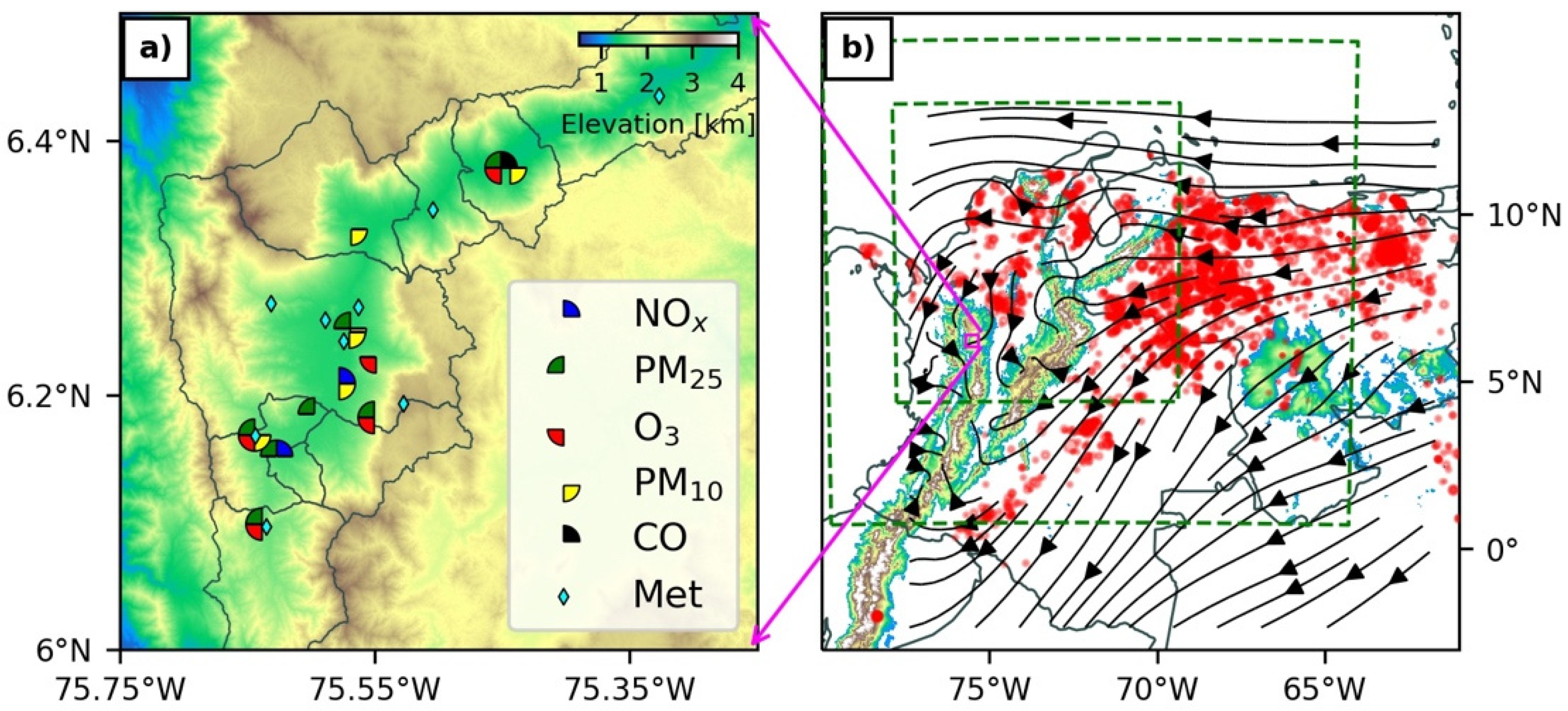
2.1. Surface Stations

Surface data come from the air quality and meteorological ground-level networks managed by the local Early Warning System in AMVA (SIATA for its Spanish acronym; https://siata.gov.co, accessed on 30 August 2021). All available air quality data that satisfy the condition of having less than 25% missing data for the period from January 2016 to June 2020 were considered for the analyses. After removing spurious data using the control flags provided by SIATA, seven stations for PM2.5, five for PM10 and O3, two for NOx (nitric oxide—NO—and NO2), and one for carbon monoxide (CO) at hourly frequency were considered for the analyses (Figure 1).
The same screening was applied to the meteorological network, leaving nine stations to analyze surface temperature, relative humidity, and precipitation, and seven stations for wind speed. The meteorological network data (one-minute frequency) were averaged to the hourly resolution of the air quality data.
Details about the percentage of no-data voids, gaps, and sample size of the final datasets are presented in Supplementary Tables S1 and S2.

2.2. Traffic Data

Local traffic information was used to determine the effect of the lockdown on vehicle intensity (total number of vehicles per hour). We obtained mean daily vehicle intensity from the local mobility authority (SIMM, Spanish acronym; https://www.medellin.gov.co/simm/, accessed on 30 August 2021), which is derived from 80 closed-circuit television cameras distributed around the main municipality (Supplementary Figure S1). The cameras are located around different road types, mainly in trunk, primary, and secondary roads. The information is not discretized by vehicle type, but allows the determination of changes in total traffic volumes. The percent variations in traffic during March and April 2020 were determined using the mean vehicle intensity of March–April 2016–2019 as a reference (data are available from 2016).
Changes in traffic intensity are used as a measure of the effectiveness and stringency of the implemented lockdown measures. Traffic variations are relevant for pollution levels as the transport sector largely dominates the emissions of PM, NOx, and CO, with contributions larger than 80% [24]. In addition, changes in traffic are also indicative of the effectiveness of the lockdown measures on various sectors, given that the closure of industries, schools, or universities also influences traffic volumes. However, variations in traffic intensity do not necessarily result in a proportional (linear) variation in traffic emissions, and the lockdown measures affected many sectors that also contribute to pollutant emissions. To determine changes in emissions for various sectors requires information that is not available, is difficult to obtain, and is highly uncertain under lockdown conditions. The use of traffic variation is thus not intended to explain all the changes in pollutant levels, but is just an indicator of the lockdown measures that is determined with high confidence.

2.3. Fire Activity

Fire activity data are based on the Moderate Resolution Imaging Spectroradiometer (MODIS) Collection 6 active fire products, with a horizontal resolution of 1 km [25]. We analyzed daily total fire radiative power (FRP) and active fire (“hotspots”) counts in the domain (Figure 1b), using measurements with detection confidence levels (provided in the data) of 90% or larger (high confidence of being real fires). The MODIS active fire product has been previously used for air quality analysis in the region [9,20,26].
In addition, the VIIRS (Visible Infrared Imaging Radiometer Suite) active fire product, with a resolution of 375 m [27], was used for dispersion modeling (described below). We included data with high and nominal detection confidence and removed low confidence data, i.e., detections with potential daytime sun glint contamination and low relative temperature anomalies. The VIIRS product was selected for dispersion modeling as it has a better spatial resolution, which has been identified as important for having lower fire detection errors than MODIS in other areas of the world [28]. Further details of the use of VIIRS FRP for dispersion modeling are provided below. MODIS and VIIRS data were obtained from the Fire Information for Resource Management System platform (FIRMS; https://firms.modaps.eosdis.nasa.gov/, accessed on 30 August 2021).

2.4. Effects of Lockdown on Pollutant Levels

The analyses of the lockdown effects on air quality around the world have been conducted with different approaches, including comparisons of lockdown with pre-lockdown periods of weeks (e.g., [29]), months (e.g., [30]), and years (e.g., [20]), using both satellite and surface data sources (e.g., [12]). The use of previous years as a reference to determine lockdown impacts aims to account for the effects of meteorological conditions and trends on air quality, although anomalous weather conditions during the periods of interest are not completely incorporated. In order to disentangle the actual effects of the lockdown on pollution levels, a variety of methods have been applied, including multivariate regression analysis methods and machine learning [11]. Although there are uncertainties in these methods and the effects of meteorology may not be fully taken into account, methods such as multiple linear regression and random forest regression have been proven satisfactory for such a purpose (e.g., [12,23]).
To account for the effects of meteorology while considering the underlying assumptions and uncertainties of different methods, we used three different methods to determine pollutant variations during the periods of interest.
First is a comparison with previous years to explore interannual variability: variations for the periods of interest are determined relative to the same season of the lockdown (March–April) during the previous four years (2016–2019).
Second, the machine-learning algorithm random forest regression (RF; [31]) was used to predict the “business as usual” (without the lockdown) pollution levels for the periods of interest. RF approaches have been used for analyzing the effects of the COVID-19 lockdown on air quality [23,32,33] and for taking into account the effects of meteorology on different air quality data analyses (e.g., [34,35,36]).
The following predictive variables were included to train the RF: relative humidity, temperature, precipitation (afternoon and nighttime), atmospheric pressure, wind velocity and direction, incoming solar radiation, Julian day, year, weekday, and days since 1 January 2000 (as a trend term). Meteorological and air quality data were resampled from hourly to daily values using daily averages (except from precipitation that was accumulated), removing days with less than 75% valid data. The nearest meteorological station was assigned to air quality stations without meteorological data.
In addition, regional fire information from the MODIS active fire product was included as an explanatory variable to account for the variability associated with the regional transport of biomass burning emissions. We performed a preliminary analysis of the total number of daily detected fires (“hotspots”) and the daily sum of FRP, considering lags from 1 up to 5 days for representing the transport time of regional biomass burning emissions. Based on the importance of the predictive variables in the RF algorithm (not shown), only the daily sums of FRP for lags of 3, 4, and 5 days were used as explanatory variables.
A forest (RF) was constructed for each pollutant of interest as a target variable: PM2.5, PM10, NO2, NO, O3, and CO. Following previous studies, 300 trees were used in the RF algorithm. The selected training period is from January 2016 to December 2019, and a random sample of 20% of the data was extracted for validation. The trained RF regression was used to predict the pollution levels from January 2020 to June 2020. Finally, to determine variations in pollution levels associated with the lockdown, the predicted “business as usual” pollution levels of the RF model (expected levels) were compared to the observed levels (actual levels).
Third, a multiple linear regression (MLR) model was also implemented to account for the effects of meteorology, following Venter et al. [12]. Individual MLR models were built for each pollutant and monitoring station, using the same explanatory variables and data used in the RF regression models. The variations in pollution levels using the MLR models were determined as those with the RF regression model.

2.5. Transport of Biomass Burning Emissions

The transport of biomass burning emissions is studied using a Lagrangian Stochastic Particle Dispersion Model (LSPDM), in which particles released from active fires detected by VIIRS are dispersed using forward trajectories. The implemented modeling framework (described below) is integrated from April 10 to 20, a period of reduced vehicle intensity related to lockdown measures and relatively high fire activity in the region.
Meteorological fields for driving the dispersion model were obtained with the Weather Research and Forecasting (WRF) model version 4.1.1, using two one-way nested domains with horizontal grid spacings of 12 km in the outer domain (D1; 146 × 136 grid cells) and 4 km in the inner domain (D2; 235 × 250 grid cells). D1 extends from about 1–15 North and 64–80 West, and D2 from 4–13 North and 69–78 West. The model top is fixed at 50 hPa with 65 full sigma vertical levels. Initial and boundary conditions (updated every 3 h) come from the European Center for Medium-Range Weather Forecasts’ ERA5 reanalysis, at 0.25° grid sizes [37,38]. The chosen physical parameterization schemes are: MYJ for planetary boundary layer; Dudhia and RRTM for shortwave and longwave radiation, respectively; Thompson for microphysics; Grell–Devenyi for convection; Janjic Eta for surface layer; and the Noah-MP land surface model.
For the dispersion of biomass burning emissions, we used the LSPDM developed at the Desert Research Institute [39], which has been previously adapted to receive meteorological fields from WRF [8]. Emissions are generated for all grid cells that present active fires in the VIIRS data using the FRP. FRP has been widely used to estimate biomass burning emissions, including the Quick Fire Emissions Dataset (QFED; [40]) and the Global Fire Assimilation System (GFAS; [41]), assuming a direct relationship between FRP and biomass burning rate [42].
From the 35,649 fires detected by VIIRS during the modeling period, 30,761 that had nominal or high confidence are considered, mainly occurring between April 13 and 16 (Supplementary Table S3). As the resolution of VIIRS is higher than that of WRF, the total FRP from all fires detected inside a WRF grid cell is computed. FRP values for every grid cell are updated at each satellite overpass over the study area (12 h), occurring around 05 and 17 UTC. Particles are released from emitting grid points (non-zero FRP) with an injection function using a histogram of 10 equally spaced classes. The total numbers of particles released during the simulations are 311,130 and 380,900 for domains D1 and D2, respectively. Particle injection height, essential for the simulation of biomass burning emissions transport [43], is determined using the plume rise model of Sofiev et al. [44] for wild-land fires. The method is based on energy balance and dimensional analysis, using satellite data to constrain the developed equation. The predicted injection height uses the FRP to describe the buoyant source, readily available from VIIRS, and meteorological conditions at the place of the fire, derived from WRF: the Brunt–Vaisälä frequency and the boundary layer height. Gravitational settling and deposition processes are not considered in this version of the model.

3. Results

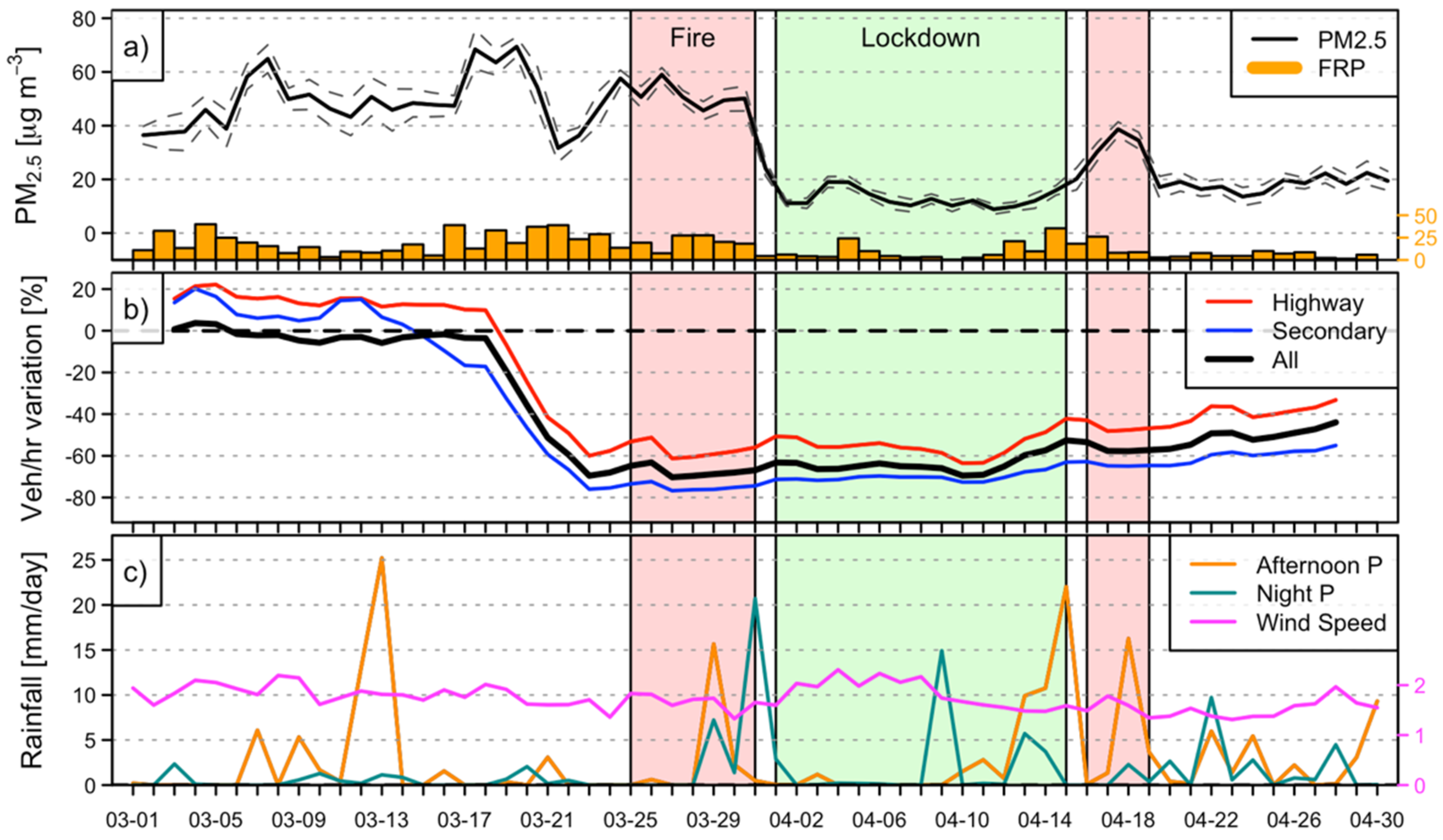
3.1. Lockdown and Fire Periods

To disentangle the effects of the implemented lockdown restrictions from those related to fire activity during the lockdown, we defined periods of interest considering the legislative measures, the resulting traffic variations (vehicle intensity), regional fire activity, and concentrations of fine particulate matter (the critical pollutant in AMVA) during March and April 2020.
Figure 2 shows the average PM2.5 concentrations, the vehicle intensity variation, the total daily fire counts, precipitation, and wind speed for March and April 2020. Vehicle intensity remained comparable to previous years for the first two weeks of March. A mild reduction in mean vehicle intensity is observed from 13 March for lower-order roads (blue line), when the closure of schools and universities was declared. A larger reduction in mean vehicle intensity (~70%) occurred for the weekend of 20 to 23 March, when a regional lockdown was declared. This lockdown was relaxed on 24 March before the national lockdown that started on 25 March, at 00:00 h local time. During the last week of March, at the beginning of the lockdown, PM2.5 concentrations remained high despite the large reduction in vehicle intensity (~70%), coinciding with a period of high fire activity. High PM levels were also reported in Bogotá for that period [20]. Accordingly, we defined a lockdown period from April 1 to 14 (green in Figure 2) when fire activity was relatively low and the vehicle intensity reduction was relatively steady around 70%; hereafter, we refer to this period as “Lockdown” and we use it to determine the effects of the lockdown on pollutant levels. A second period with approximately the same traffic variations of the lockdown, but when PM2.5 levels were much larger and with a higher variability, is defined from 25 to 30 March and 16 to 19 April (red in Figure 2), hereafter referred to as the “Fire” period. As suggested by Mendez-Espinosa et al. [20] and the regional fire activity data, this period can be used to analyze the effects of the regional transport of biomass burning emissions on local air quality. Although traffic counts are slightly larger for the second part of the Fire period than during the Lockdown period (~60% vs. ~70% reduction), traffic variation of about 10–15% alone and meteorological conditions (Figure 2c) cannot explain the variability in pollution levels between periods.

3.2. Meteorological Conditions and Fire Activity

We analyzed meteorological variables and regional fire activity for the periods of interest compared to the 2016–2019 March–April reference. Surface temperature and relative humidity during the Lockdown period present similar values to the reference (Supplementary Figure S2). However, there are statistically significant differences between the periods of interest and the reference. Only precipitation during the Lockdown period and wind speed during the Fire period do not show statistically significant differences (Supplementary Table S4).
The distribution of surface wind speed, mean daily rainfall rates, and total FRP is shown in Figure 3. The 2020 periods are characterized by: (1) slightly larger wind speeds relative to 2017–2019 and similar values to 2016, resulting in a mean increase between 0.1 and 0.2 m/s for the 2020 periods relative to the reference period (Figure 3a); (2) less rainfall as compared to 2017–2019, with mean daily rainfall rates comparable to 2016, the driest year from the reference (Figure 3b); and (3) an enhanced fire activity, especially before and several days after the lockdown declaration (Figure 3c), which affects air quality. Some variability can be expected from the drier conditions in 2020, but the potential effects on air quality are difficult to assess and depend on the pollutant analyzed. For example, enhanced radiation from the drier conditions could increase ozone production, but at the same time, it favors the development of a deeper boundary layer, enhancing pollutant ventilation out of AMVA [6]. The drier conditions also reduce the sink of PM2.5 by wet deposition, although the net effect depends (in AMVA) on the timing of rainfall [7].

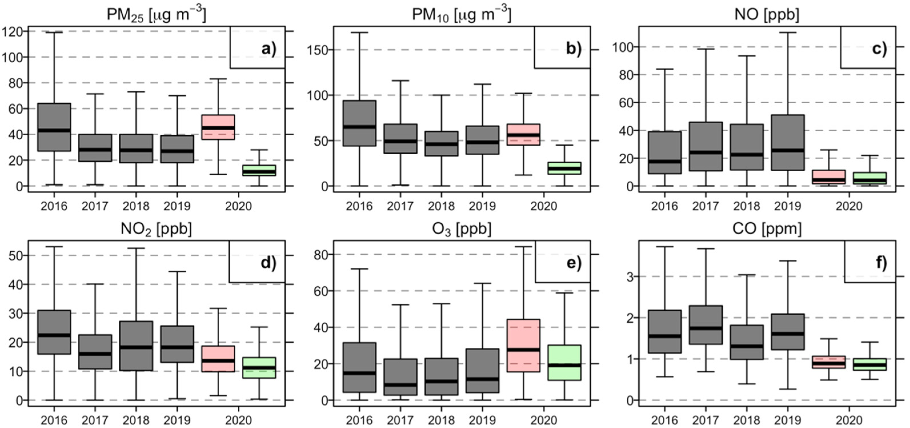
3.3. Changes in Pollutant Concentrations

Figure 4 presents the distribution of pollutant concentrations for the 2016–2019 reference period and the 2020 Lockdown and Fire periods. Relative to the reference, all pollutants but ozone showed reductions during the Lockdown period (green boxplots), with the increase in ozone mainly occurring for values in the lower range. During the Fire period, there are reductions in NOx and CO (red boxplots), but with slightly larger values as compared to the Lockdown period. However, despite the large reduction in vehicle intensity during the Fire period, there is no change in PM10 and relatively large increases in PM2.5 and O3, as compared to the reference period. All pollutants had statistically significant differences between the reference period and the Lockdown and Fire periods (Supplementary Table S4).
Three different methods were implemented to determine variations in pollution levels to account for both the uncertainty inherent to each method and the role of meteorology on air quality. First, we present the results of the ability of MLR models and RF regression to predict pollution levels during the periods of interest.
The performance of the RF and MLR models is presented in Table 1, using the root mean square error (RMSE) and the coefficient of determination (R2), which are calculated for the validation subset. In general, the RF models perform better than the MLR models for all predicted pollutants (lower RMSE and higher R2). Previous studies using both methods have also reported better performances for the RF method [45,46], related to the ability of RF to represent non-linear relationships, making multiple predictions using multiple combinations of the dependent variables. However, a better performance for MLR has also been reported [12].
The RF models have R2 scores larger than 0.5 (Table 1 and Supplementary Table S5), with higher values for O3 and PM and lower values for CO and NOx. Lower scores for CO and NOx can be explained by the locations of the measuring sites in traffic-loaded sites, which also resulted in lower scores in Lovric et al. (2021). The moderate R2 scores indicate that the models are not able to explain all the temporal variability, but are comparable to previous studies [12,23,35] and are considered reasonable to obtain reliable “business as usual” predictions during the periods of interest. Despite the larger RMSE values and the lower R2 scores in the MLR models, the average predicted values obtained with the RF and MLR models are similar for the periods of interest (Figure 5 and Table 2). However, for different applications where predictions are performed for longer periods and with larger variability in meteorological parameters, the differences in performance are expected to have a significant impact on predictions.
The results of the RF and MLR modeling suggest that the implemented measures during the Lockdown period, with a major reduction in vehicle intensity (~70%), resulted in large reductions in the mean concentrations of particulate matter, nitrogen oxides, and carbon monoxide, but ozone concentrations increased (Table 2 and Figure 6). The largest reduction occurred for NO (−76%), suggesting a proportional relationship with the reduction in traffic. The reductions in PM2.5 were between −50 and −63%, and between −59% and −64% for PM10, depending on the method. For PM, lower reductions were obtained when accounting for the effects of meteorology compared to the reductions with the reference of previous years. CO and NO2 had lower reductions, between −40% and 47% and between −43% and −47%, respectively. In contrast, O3 concentrations increased by 19% to 22%.
During the Lockdown period, NO, NO2, O3, and PM10 showed small sensitivity to the method used to calculate the variations (<5%), but larger differences occur for PM2.5 and CO. Importantly, the sensitivity between methods seems to be unrelated to the scores and errors obtained by the models (e.g., lower scores for NO than for PM2.5 in Table 1).
For the Fire period, as the idea is to explore the effects of fire activity on pollutant concentrations, the FRP values were replaced with the median of the entire dataset in the MLR and RF models. During this period, with large reductions in vehicle intensity (~60%) but relevant fire activity, mean PM2.5 concentrations were between 31% and 143% larger than the expected values under no lockdown (Figure 6b). The variations in PM2.5 are much lower when calculated with the reference of previous years, as this reference considers values for March and April, a period with significant fire activity (Figure 3c). In contrast, the larger increases when using the RF and MLR values are due to removing the fire influence for the Fire period. Similarly, PM10 concentrations showed little variation using the reference of previous years (+1%), but increased by 24% and 27% when using the RF and MLR models, respectively. O3 also increased by between 79% and 102%, despite reductions in ozone precursors: NO (−71 to −75%), NO2 (−31 to −35%), and CO (−35% to −45%) (Figure 6b). Again, variations with the MLR and RF methods are larger than with the reference of previous years due to removing the fire influence in these models, which highlights the importance of accounting for meteorological effects.
The sensitivity of the percent variation to the selected method is larger during the Fire than during the Lockdown period, probably due to the complications of the added variance from the fire activity and the absence of the actual fire conditions in the models for the Fire period. In particular, PM2.5, PM10, and O3 show, in that specific order, larger sensitivities to the selected method.
In addition, we trained another RF model for PM2.5 that does not include fire-related explanatory variables (RF-NoFire) and compared it with the standard RF model (RF-Fire) to examine the influence of fire activity on pollutant levels during the Fire period.
Figure 7 shows the time series of observed PM2.5 and the predictions with both RF models. Values are standardized (subtracting the mean and dividing by the standard deviation) to better compare lockdown observations and “business as usual” predictions. An interesting result is that when the RF model includes fire as a dependent variable, the peak in the observations during the latter part of the Fire period is also present in the predictions, whereas the predictions with the model that does not consider fire miss this peak, suggesting a direct effect of long-range biomass burning emissions in modulating pollution levels in AMVA.

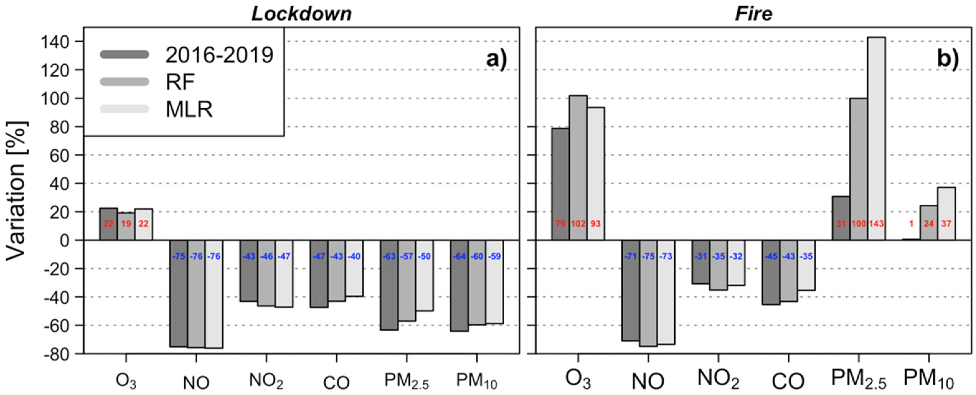
3.4. Attribution of Fire Effects on Pollutant Levels

During the Fire period, the results shown above suggest that despite the lockdown measures, with large decreases in traffic levels and, therefore, in emissions, PM2.5 (the critical pollutant in AMVA) concentrations were above normal levels (business as usual). To better identify the influence of regional biomass burning emissions, we performed a trajectory analysis using an LSPDM model. Particles were released from active fires (“hotspots”) proportionally to the FRP and later dispersed using forward trajectories. This modeling framework allows the quantification of the number of particles emitted from active fires that reach AMVA and their source location.
An evaluation of the meteorological model performance was carried out for surface wind speed and wind direction at five locations, and for upper air (500 and 700 hpa) at one location (Supplementary Figures S3 and S4). The model presented an adequate performance of surface wind speed, with a good representation of the day-to-day variability and the diurnal cycles, with an RMSE between 1.2 and 2.2 m/s (exceeding 2 m/s only at one location). For surface wind direction, there are relatively larger errors at some locations, with mean-absolute errors (MAE) between 28 and 90 degrees.
Figure 8 shows the time series of observed PM2.5 surface concentrations and fire-related particle number concentrations reaching AMVA’s air basin for dispersion simulations using the two domains shown in Figure 9. Of note is that the dispersion of particles from active fires in domain D2 shows a peak in the number of particles that reach AMVA on April 15, which coincides with an increase in observed PM2.5 concentrations. However, the modeled trajectories arrive 1–2 days earlier and last shorter than the observations. The dispersion simulation for the bigger domain (D1) shows a peak in the number of particles reaching AMVA collocated with the maximum of PM2.5 observations (April 17), suggesting that areas further away also contribute to pollution in AMVA (domain D1 is bigger than D2). However, this simulation presents an earlier and more prominent peak that was not observed in the monitoring stations.
Figure 9 shows the particle contribution of each fire episode reaching AMVA and the accumulated particle number concentration for both simulations. For D2, the largest contribution comes from the northeast of AMVA, near Venezuela, accounting for about 15% of all particles reaching AMVA (red circle in Figure 9a). There are important contributions from the lowlands north of AMVA, southeast of AMVA in the Andes, and across the border with Venezuela, near Lake Maracaibo. For domain D1 and focusing on the period where PM2.5 observations increase (April 15–20), there are many sources at longer distances to the east, across the border with Venezuela (Figure 9b), highlighting the role of long-range transport in adding variability to air quality in AMVA.
The accumulated particle number concentrations (Figure 9c,d) are largest for the lowlands, close to the areas where most fires occurred. For areas located at higher elevations, including AMVA and other inter-Andean valleys, there are much lower particle number concentrations. Although particles released from fires at long distances can reach AMVA´s air basin and contribute to pollution (shown above), smoke transport from the sources is challenging, with the Andes mountains providing a natural barrier. For example, most of the smoke from the large fires in Venezuela (maximum concentrations in Figure 9d) is transported to the southeast by the Orinoco low-level jet (recall Figure 1b) and remains east of the Andes foothills, consistent with previous studies [47,48]. However, as shown before, vegetation fires from this area can also contribute to pollution in AMVA and help explain the higher concentrations for the larger domain D1, relative to D2 (Figure 9c,d).

4. Discussion

Our results show that, during the Lockdown period, large average reductions occurred in almost all the analyzed pollutants (PM2.5: −50% to −63%, PM10: −59% to −64%, NO: −75% to −76%, NO2: −43% to −47%, and CO: −40% to −47%), but the average O3 concentration increased (19% to 22%). The range in values corresponds to variations being calculated using three different methods, which resulted in relatively similar variations for most pollutants, especially between calculations with the RF and MLR models. These results agree with those of Lovric et al. [23], who found similar variations for calculations using historical (reference) data and RF predictions for the city of Graz, Austria.
The variations reported in Mendez-Espinosa et al. [20] for AMVA, relative to this study, are larger for NO2, as their results show reductions of 69%, but are smaller for particulate matter: 6% to 36% for PM2.5, and 33% for PM10. These differences arise from the definition of the lockdown period, as they defined the lockdown from March 20 to April 26, the fact that there were less stations included in their case, and the methods used for the variation calculations. Relative to other studies in South America, our results show larger reductions in PM2.5 and PM10 [15,17,19], relatively close to those reported in Lima (PM2.5: −43%; PM10: −58%) [16], but the variations for O3 reported here were lower, only relatively close to the 30% increase for Sao Paulo [19] and far from the 60% increase in Santiago and Lima [15,16].
The variations in pollutants reported here are not only related to the described changes in traffic, but are also influenced by all sectors contributing to emissions, which were also impacted by the implemented measures. However, the contributions by other sectors should be much lower than those of transportation, which largely dominates emissions (over 80% for PM and NOx) [24]. Another relevant consideration for the calculated variations is that the Lockdown period (April 1 to 14) falls between the two Fire periods (March 25 to 30 and April 16 to 19), and pollution levels during the first Fire period may have had an effect in the lockdown period (background concentrations).
The large reductions in particulate matter during the Lockdown period indicate that much healthier levels are reachable in AMVA, with an average PM2.5 (PM10) concentration of 13 (20) μg/m3. PM concentrations reached values close to the World Health Organization annual mean guidelines (10 and 20 μg/m3 for PM2.5 and PM10, respectively). However, reductions in emissions that are comparable to the lockdown require significant efforts from decision-makers and society.
In the case of ozone, it is of particular importance that despite the large reduction in NOx during the Lockdown period, mean daily concentrations increased. This ozone increase is related to the weakening of ozone titration by NO, the large reduction in PM2.5 that can reduce the sink of hydroperoxy radicals (see, e.g., [49]), or even due to higher emissions of VOCs from increases in the use of household cleaning products [14]. Given that reductions in NOx are probable in the future, it is necessary to further investigate the ozone regime in AMVA and consider, for example, the potential effects of urban vegetation in the production of biogenic VOCs and, hence, on air quality (see, e.g., [50]).
The Fire period highlighted the large effect that regional biomass burning emissions have on the air quality of AMVA, especially for particulate matter and ozone, which resulted in larger concentrations despite a considerable reduction in mobile emissions (~70% reduction in mean vehicle intensity). Biomass burning emissions have been observed to cause a high impact on ozone and particulate matter in urban areas at large distances from fires in different regions of the world [51,52,53,54,55]. An important reason is that vegetation fires are major sources of organic carbon and black carbon particles, and NOx and VOCs (e.g., [56]). Dispersion modeling with the LSPDM shows that emissions from fires over 1000 km away in Venezuela can reach AMVA and increase pollution levels. This is evident when comparing simulations for both domains, as the more extensive D1 domain results in a larger number of particles reaching AMVA. However, differences between simulations can also be related to the horizontal resolution of each domain, which is known to influence the simulation of smoke transport [21], as it results in a smoother topography for D1 and also affects model meteorology in inter-Andean valleys [8,22]. Differences between simulations and observations in AMVA can be related to limitations in the dispersion model, such as the lack of interactions with clouds and rainfall, chemical processes, uncertainties in modeled meteorology, among others. Even though relationships between fire-related emissions and detrimental air quality conditions have been suggested for the region, we have shown that establishing direct connections to day-to-day variability is challenging. Further research is needed to understand the smoke pathways and depositional processes, together with the emissions and lifespan of the smoke constituents and their chemical and physical interaction with AMVA pollutant precursors. These challenges for the simulation and forecast of smoke transport are consistent with the state of the art [21].
The significant influence of regional fire activity on air quality in AMVA, even under conditions of large reductions in local emissions, implies that air pollution cannot be treated locally alone, highlighting the importance of biomass burning emissions on transboundary air quality management, as discussed in Bergin et al. [51]. Measures to reduce emissions and improve air quality in urban areas in Colombia need to be accompanied by measures for monitoring and managing fire activity in Northern South America and the Amazon [10]. The long-range transport of pollutants affecting AMVA, related to Saharan dust aerosols and fire plumes [20,55], is a trackable and observable characteristic that can be monitored and predicted for producing early warnings of air quality and informing management strategies.

5. Conclusions

The lockdown measure was intended as a strategy to contain or reduce the spread of the COVID-19 pandemic. However, its restrictions on transportation provided a unique opportunity to study the impacts on air quality in a metropolitan and highly urbanized area such as Medellín and its metropolitan area, Colombia. We determined variations in pollution levels using three different methods, a reference of previous years, and predictions of “business as usual conditions” with multiple linear regression models and random forest models, which are largely independent of meteorological conditions and interannual variability. The implemented lockdown largely reduced economic and social activities, showing a reduction in mean vehicle intensity of 70%. As a result of the lockdown, the random forest method produced percent variations for PM2.5, PM10, NO, NO2, CO, and O3 of −57%, −60%, −76%, −46%, −43%, and +19%, respectively, when regional fire activity exerted a low influence on local air quality conditions. However, high fire activity during the lockdown resulted in particulate matter and ozone levels larger than the reference and predicted “business as usual” values, shadowing the effects of the lockdown and highlighting the important role of regional fire activity and the long-range transport of biomass burning emissions in adding variability to air quality in AMVA.
The natural opportunity created by government responses to the pandemic proved that the necessity to achieve healthier air pollution levels is possible in AMVA, but important challenges remain: (1) effective measures do not only require significant reductions in the emissions from transportation and industry, but should also consider the effects of regional fire activity; (2) while municipal authorities in AMVA can decide about these restrictions at the local level, they can barely decide about important factors affecting fire activity at the regional level, which poses challenges in the context of transboundary air quality management; and (3) effective measures to reduce ozone levels should not be expected from measures that are effective in reducing nitrogen oxides and particulate matter; further studies of chemical pathways for secondary pollutants are required.

Supplementary Materials

The following are available online at https://www.mdpi.com/article/10.3390/atmos12091137/s1, Figure S1: Location of the 80 traffic cameras used and the main road network, Figure S2: Boxplots of (a) relative humidity (RH) and (b) temperature (T) for March–April 2016–2019 (gray) and the 2020 Fire (pink) and Lockdown (green) periods, Figure S3: Time series of modeled and observed 10-m wind speed (left panels) and wind direction (right panels) for different locations in the dispersion model domain. The location of the stations is shown in Figure S5. Model values for the closest model pixel. Annotated text values in blue show the RMSE for wind speed and the MAE for wind direction, respectively, Figure S4: Time series of modeled wind speed and wind direction at 500 and 700 hpa, at the grid cell closest to El Dorado Airport (Figure S5). Black points (stars) show observations from radiosondes launched from the airport daily at 12Z, Figure S5: Location of the stations used for the model evaluation of Supplementary Figure S3, Table S1: Characteristics of the air quality dataset after data processing (January 2016 to June 2020). Samples indicate the number of valid hourly values (included in the analysis); NA % represents the percentage of no-data voids (NA); and Gaps indicate the largest three consecutive values of NA (hourly values), Table S2: As Table S1 but for meteorological variables. RH: relative humidity; T temperature; P: precipitation; Pres: atmospheric pressure; WS: wind speed; WD: wind direction, Table S3: Details about the final dataset of FRP and fire (hotspots) counts, Table S4: Kolmogorov–Smirnov test for meteorological and air quality variables, Table S5: Metrics calculated for the validation set, i.e., random sample of 20% of the 2016–2019 dataset.

Author Contributions

Conceptualization, J.J.H., J.F.M., J.F.S. and A.M.R.; methodology, J.J.H., with contributions by all authors; software, J.F.M., J.J.H. and K.S.H.; validation, J.J.H., J.F.M., K.S.H. and P.A.G.-R.; formal analysis, J.J.H., K.S.H., P.A.G.-R. and V.R.; investigation, J.J.H., K.S.H. and P.A.G.-R.; resources, J.F.M.; data curation, J.J.H. and K.S.H.; writing—original draft preparation, J.J.H.; writing—review and editing, J.J.H. with contributions by all authors; visualization, J.J.H. with contributions by all authors; supervision, J.F.M., J.F.S. and A.M.R. All authors have read and agreed to the published version of the manuscript.

Funding

J.J.H. was funded by the Colombian Ministry of Science & Technology and Innovation (MINCIENCIAS), under the national doctoral grant 727-2015. J.F.M. was supported by the Desert Research Institute. J.A.P.-M. was funded by the Colombian Ministry of Science, Technology and Innovation (MINCIENCIAS) through program “Excelencia doctoral del Bicentenario” grant 20230017-25-2020.

Institutional Review Board Statement

Not applicable.

Informed Consent Statement

Not applicable.

Data Availability Statement

Air quality and meteorological data were obtained from SIATA: https://siata.gov.co/descarga_siata/index.php/index2 (accessed on 30 August 2021). Vehicle intensity data were obtained from SIMM: https://www.medellin.gov.co/simm/ (accessed on 30 August 2021). MODIS and VIIRS data were obtained from the FIRMS: https://firms.modaps.eosdis.nasa.gov/ (accessed on 30 August 2021).

Acknowledgments

We thank two anonymous reviewers for providing comments that significantly improved this paper.

Conflicts of Interest

The authors declare no conflict of interest.

References

  1. Forouzanfar, M.H.; Afshin, A.; Alexander, L.T.; Anderson, H.R.; Bhutta, Z.A.; Biryukov, S.; Brauer, M.; Burnett, R.; Cercy, K.; Charlson, F.J.; et al. Global, Regional, and National Comparative Risk Assessment of 79 Behavioural, Environmental and Occupational, and Metabolic Risks or Clusters of Risks, 1990–2015: A Systematic Analysis for the Global Burden of Disease Study 2015. Lancet 2016, 388, 1659–1724. [Google Scholar] [CrossRef] [Green Version]
  2. Lelieveld, J.; Pozzer, A.; Pöschl, U.; Fnais, M.; Haines, A.; Münzel, T. Loss of Life Expectancy from Air Pollution Compared to Other Risk Factors: A Worldwide Perspective. Cardiovasc. Res. 2020, 116, 1910–1917. [Google Scholar] [CrossRef] [PubMed]
  3. Chowdhury, S.; Pozzer, A.; Dey, S.; Klingmueller, K.; Lelieveld, J. Changing Risk Factors That Contribute to Premature Mortality from Ambient Air Pollution between 2000 and 2015. Environ. Res. Lett. 2020, 15, 074010. [Google Scholar] [CrossRef]
  4. Gerten, C.; Fina, S.; Rusche, K. The Sprawling Planet: Simplifying the Measurement of Global Urbanization Trends. Front. Environ. Sci. 2019, 7, 140. [Google Scholar] [CrossRef]
  5. Crippa, M.; Guizzardi, D.; Muntean, M.; Schaaf, E.; Dentener, F.; van Aardenne, J.A.; Monni, S.; Doering, U.; Olivier, J.G.J.; Pagliari, V.; et al. Gridded Emissions of Air Pollutants for the Period 1970–2012 within EDGAR v4.3.2. Earth Syst. Sci. Data 2018, 10, 1987–2013. [Google Scholar] [CrossRef] [Green Version]
  6. Herrera-Mejía, L.; Hoyos, C.D. Characterization of the Atmospheric Boundary Layer in a Narrow Tropical Valley Using Remote-Sensing and Radiosonde Observations and the WRF Model: The Aburrá Valley Case-Study. Q. J. R. Meteorol. Soc. 2019, 145, 2641–2665. [Google Scholar] [CrossRef]
  7. Roldán-Henao, N.; Hoyos, C.D.; Herrera-Mejía, L.; Isaza, A. An Investigation of the Precipitation Net Effect on the Particulate Matter Concentration in a Narrow Valley: Role of Lower-Troposphere Stability. J. Appl. Meteorol. Climatol. 2020, 59, 401–426. [Google Scholar] [CrossRef]
  8. Henao, J.J.; Mejía, J.F.; Rendón, A.M.; Salazar, J.F. Sub-Kilometer Dispersion Simulation of a CO Tracer for an Inter-Andean Urban Valley. Atmos. Pollut. Res. 2020, 11, 928–945. [Google Scholar] [CrossRef]
  9. Mendez-Espinosa, J.F.; Belalcazar, L.C.; Morales Betancourt, R. Regional Air Quality Impact of Northern South America Biomass Burning Emissions. Atmos. Environ. 2019, 203, 131–140. [Google Scholar] [CrossRef]
  10. Ballesteros-González, K.; Sullivan, A.P.; Morales-Betancourt, R. Estimating the Air Quality and Health Impacts of Biomass Burning in Northern South America Using a Chemical Transport Model. Sci. Total Environ. 2020, 739, 139755. [Google Scholar] [CrossRef]
  11. Gkatzelis, G.I.; Gilman, J.B.; Brown, S.S.; Eskes, H.; Gomes, A.R.; Lange, A.C.; McDonald, B.C.; Peischl, J.; Petzold, A.; Thompson, C.R.; et al. The Global Impacts of COVID-19 Lockdowns on Urban Air Pollution: A Critical Review and Recommendations. Elem. Sci. Anthr. 2021, 9. [Google Scholar] [CrossRef]
  12. Venter, Z.S.; Aunan, K.; Chowdhury, S.; Lelieveld, J. COVID-19 Lockdowns Cause Global Air Pollution Declines. Proc. Natl. Acad. Sci. USA 2020, 117, 18984–18990. [Google Scholar] [CrossRef] [PubMed]
  13. Chauhan, A.; Singh, R.P. Decline in PM2.5 Concentrations over Major Cities around the World Associated with COVID-19. Environ. Res. 2020, 187, 109634. [Google Scholar] [CrossRef]
  14. Kroll, J.H.; Heald, C.L.; Cappa, C.D.; Farmer, D.K.; Fry, J.L.; Murphy, J.G.; Steiner, A.L. The Complex Chemical Effects of COVID-19 Shutdowns on Air Quality. Nat. Chem. 2020, 12, 777–779. [Google Scholar] [CrossRef]
  15. Toro, A.R.; Catalán, F.; Urdanivia, F.R.; Rojas, J.P.; Manzano, C.A.; Seguel, R.; Gallardo, L.; Osses, M.; Pantoja, N.; Leiva-Guzman, M.A. Air Pollution and COVID-19 Lockdown in a Large South American City: Santiago Metropolitan Area, Chile. Urban Clim. 2021, 36, 100803. [Google Scholar] [CrossRef] [PubMed]
  16. Rojas, J.P.; Urdanivia, F.R.; Garay, R.A.; García, A.J.; Enciso, C.; Medina, E.A.; Toro, R.A.; Manzano, C.; Leiva-Guzmán, M.A. Effects of COVID-19 Pandemic Control Measures on Air Pollution in Lima Metropolitan Area, Peru in South America. Air Qual. Atmos. Health 2021, 14, 925–933. [Google Scholar] [CrossRef]
  17. Zalakeviciute, R.; Vasquez, R.; Bayas, D.; Buenano, A.; Mejia, D.; Zegarra, R.; Diaz, V.; Lamb, B. Drastic Improvements in Air Quality in Ecuador during the COVID-19 Outbreak. Aerosol Air Qual. Res. 2020, 20, 1783–1792. [Google Scholar] [CrossRef]
  18. Zambrano-Monserrate, M.A.; Ruano, M.A. Has Air Quality Improved in Ecuador during the COVID-19 Pandemic? A Parametric Analysis. Air Qual. Atmos. Health 2020, 13, 929–938. [Google Scholar] [CrossRef]
  19. Nakada, L.Y.K.; Urban, R.C. COVID-19 Pandemic: Impacts on the Air Quality during the Partial Lockdown in São Paulo State, Brazil. Sci. Total Environ. 2020, 730, 139087. [Google Scholar] [CrossRef]
  20. Mendez-Espinosa, J.F.; Rojas, N.Y.; Vargas, J.; Pachón, J.E.; Belalcazar, L.C.; Ramírez, O. Air Quality Variations in Northern South America during the COVID-19 Lockdown. Sci. Total Environ. 2020, 749, 141621. [Google Scholar] [CrossRef]
  21. Ye, X.; Arab, P.; Ahmadov, R.; James, E.; Grell, G.A.; Pierce, B.; Kumar, A.; Makar, P.; Chen, J.; Davignon, D.; et al. Evaluation and Intercomparison of Wildfire Smoke Forecasts from Multiple Modeling Systems for the 2019 Williams Flats Fire. Atmos. Chem. Phys. Discuss. 2021, 1–69. [Google Scholar] [CrossRef]
  22. Posada-Marín, J.A.; Rendón, A.M.; Salazar, J.F.; Mejía, J.F.; Villegas, J.C. WRF Downscaling Improves ERA-Interim Representation of Precipitation around a Tropical Andean Valley during El Niño: Implications for GCM-Scale Simulation of Precipitation over Complex Terrain. Clim. Dyn. 2019, 52, 3609–3629. [Google Scholar] [CrossRef]
  23. Lovrić, M.; Pavlović, K.; Vuković, M.; Grange, S.K.; Haberl, M.; Kern, R. Understanding the True Effects of the COVID-19 Lockdown on Air Pollution by Means of Machine Learning. Environ. Pollut. 2021, 274, 115900. [Google Scholar] [CrossRef]
  24. AMVA. Plan Integral De Gestion De La Calidad Del Aire Para El Area Metropolitana Del Valle de Aburra—PIGECA. Area Metropolitana Del Valle de Aburra—Clean Air Institute—Universidad Pontificia Bolivariana. 2017. Available online: https://www.metropol.gov.co/ambiental/calidad-del-aire/Documents/PIGECA/PIGECA-Aprobado-Dic-2017.pdf (accessed on 30 August 2021).
  25. Giglio, L.; Schroeder, W.; Justice, C.O. The Collection 6 MODIS Active Fire Detection Algorithm and Fire Products. Remote Sens. Environ. 2016, 178, 31–41. [Google Scholar] [CrossRef] [PubMed] [Green Version]
  26. Rincón-Riveros, J.M.; Rincón-Caro, M.A.; Sullivan, A.P.; Mendez-Espinosa, J.F.; Belalcazar, L.C.; Quirama Aguilar, M.; Morales Betancourt, R. Long-Term Brown Carbon and Smoke Tracer Observations in Bogotá, Colombia: Association with Medium-Range Transport of Biomass Burning Plumes. Atmos. Chem. Phys. 2020, 20, 7459–7472. [Google Scholar] [CrossRef]
  27. Schroeder, W.; Oliva, P.; Giglio, L.; Csiszar, I.A. The New VIIRS 375m Active Fire Detection Data Product: Algorithm Description and Initial Assessment. Remote Sens. Environ. 2014, 143, 85–96. [Google Scholar] [CrossRef]
  28. Fu, Y.; Li, R.; Wang, X.; Bergeron, Y.; Valeria, O.; Chavardès, R.D.; Wang, Y.; Hu, J. Fire Detection and Fire Radiative Power in Forests and Low-Biomass Lands in Northeast Asia: MODIS versus VIIRS Fire Products. Remote Sens. 2020, 12, 2870. [Google Scholar] [CrossRef]
  29. Tobías, A.; Carnerero, C.; Reche, C.; Massagué, J.; Via, M.; Minguillón, M.C.; Alastuey, A.; Querol, X. Changes in Air Quality during the Lockdown in Barcelona (Spain) One Month into the SARS-CoV-2 Epidemic. Sci. Total Environ. 2020, 726, 138540. [Google Scholar] [CrossRef]
  30. Wang, X.; Zhang, R. How Did Air Pollution Change during the COVID-19 Outbreak in China? Bull. Am. Meteorol. Soc. 2020, 101, E1645–E1652. [Google Scholar] [CrossRef]
  31. Breiman, L. Random Forests. Mach. Learn. 2001, 45, 5–32. [Google Scholar] [CrossRef] [Green Version]
  32. Wang, Y.; Wen, Y.; Wang, Y.; Zhang, S.; Zhang, K.M.; Zheng, H.; Xing, J.; Wu, Y.; Hao, J. Four-Month Changes in Air Quality during and after the COVID-19 Lockdown in Six Megacities in China. Environ. Sci. Technol. Lett. 2020, 7, 802–808. [Google Scholar] [CrossRef]
  33. Zheng, H.; Kong, S.; Chen, N.; Yan, Y.; Liu, D.; Zhu, B.; Xu, K.; Cao, W.; Ding, Q.; Lan, B.; et al. Significant Changes in the Chemical Compositions and Sources of PM2.5 in Wuhan since the City Lockdown as COVID-19. Sci. Total Environ. 2020, 739, 140000. [Google Scholar] [CrossRef]
  34. Grange, S.K.; Carslaw, D.C. Using Meteorological Normalisation to Detect Interventions in Air Quality Time Series. Sci. Total Environ. 2019, 653, 578–588. [Google Scholar] [CrossRef]
  35. Grange, S.K.; Carslaw, D.C.; Lewis, A.C.; Boleti, E.; Hueglin, C. Random Forest Meteorological Normalisation Models for Swiss PM10 Trend Analysis. Atmos. Chem. Phys. 2018, 18, 6223–6239. [Google Scholar] [CrossRef] [Green Version]
  36. Vu, T.V.; Shi, Z.; Cheng, J.; Zhang, Q.; He, K.; Wang, S.; Harrison, R.M. Assessing the Impact of Clean Air Action on Air Quality Trends in Beijing Using a Machine Learning Technique. Atmos. Chem. Phys. 2019, 19, 11303–11314. [Google Scholar] [CrossRef] [Green Version]
  37. Copernicus Climate Change Service (C3S) ERA5: Fifth Generation of ECMWF Atmospheric Reanalyses of the Global Climate. Available online: https://www.ecmwf.int/en/forecasts/dataset/ecmwf-reanalysis-v5 (accessed on 30 August 2021).
  38. Hersbach, H.; Bell, B.; Berrisford, P.; Hirahara, S.; Horányi, A.; Muñoz-Sabater, J.; Nicolas, J.; Peubey, C.; Radu, R.; Schepers, D.; et al. The ERA5 Global Reanalysis. Q. J. R. Meteorol. Soc. 2020, 146, 1999–2049. [Google Scholar] [CrossRef]
  39. Mejia, J.F.; Gillies, J.A.; Etyemezian, V.; Glick, R. A Very-High Resolution (20m) Measurement-Based Dust Emissions and Dispersion Modeling Approach for the Oceano Dunes, California. Atmos. Environ. 2019, 218, 116977. [Google Scholar] [CrossRef]
  40. Darmenov, A.S.; da Silva, A.M. The Quick Fire Emissions Dataset (QFED): Documentation of Versions 2.1, 2.2 and 2.4; NASA: Washington, DC, USA, 2015. [Google Scholar]
  41. Kaiser, J.W.; Heil, A.; Andreae, M.O.; Benedetti, A.; Chubarova, N.; Jones, L.; Morcrette, J.-J.; Razinger, M.; Schultz, M.G.; Suttie, M.; et al. Biomass Burning Emissions Estimated with a Global Fire Assimilation System Based on Observed Fire Radiative Power. Biogeosciences 2012, 9, 527–554. [Google Scholar] [CrossRef] [Green Version]
  42. Li, F.; Zhang, X.; Roy, D.P.; Kondragunta, S. Estimation of Biomass-Burning Emissions by Fusing the Fire Radiative Power Retrievals from Polar-Orbiting and Geostationary Satellites across the Conterminous United States. Atmos. Environ. 2019, 211, 274–287. [Google Scholar] [CrossRef]
  43. Paugam, R.; Wooster, M.; Freitas, S.; Val Martin, M. A Review of Approaches to Estimate Wildfire Plume Injection Height within Large-Scale Atmospheric Chemical Transport Models. Atmos. Chem. Phys. 2016, 16, 907–925. [Google Scholar] [CrossRef] [Green Version]
  44. Sofiev, M.; Ermakova, T.; Vankevich, R. Evaluation of the Smoke-Injection Height from Wild-Land Fires Using Remote-Sensing Data. Atmos. Chem. Phys. 2012, 12, 1995–2006. [Google Scholar] [CrossRef] [Green Version]
  45. Xie, X.; Wu, T.; Zhu, M.; Jiang, G.; Xu, Y.; Wang, X.; Pu, L. Comparison of Random Forest and Multiple Linear Regression Models for Estimation of Soil Extracellular Enzyme Activities in Agricultural Reclaimed Coastal Saline Land. Ecol. Indic. 2021, 120, 106925. [Google Scholar] [CrossRef]
  46. Yuchi, W.; Gombojav, E.; Boldbaatar, B.; Galsuren, J.; Enkhmaa, S.; Beejin, B.; Naidan, G.; Ochir, C.; Legtseg, B.; Byambaa, T.; et al. Evaluation of Random Forest Regression and Multiple Linear Regression for Predicting Indoor Fine Particulate Matter Concentrations in a Highly Polluted City. Environ. Pollut. 2019, 245, 746–753. [Google Scholar] [CrossRef]
  47. Hernandez, A.J.; Morales-Rincon, L.A.; Wu, D.; Mallia, D.; Lin, J.C.; Jimenez, R. Transboundary Transport of Biomass Burning Aerosols and Photochemical Pollution in the Orinoco River Basin. Atmos. Environ. 2019, 205, 1–8. [Google Scholar] [CrossRef]
  48. Rodríguez-Gómez, C.; Echeverry, G.; Jaramillo, A.; Ladino, L.A. The Negative Impact of Biomass Burning and the Orinoco Low-Level Jet on the Air Quality of the Orinoco River Basin. Available online: https://www.revistascca.unam.mx/atm/index.php/atm/article/view/52979 (accessed on 30 August 2021).
  49. Li, K.; Jacob, D.J.; Liao, H.; Shen, L.; Zhang, Q.; Bates, K.H. Anthropogenic Drivers of 2013–2017 Trends in Summer Surface Ozone in China. Proc. Natl. Acad. Sci. USA 2019, 116, 422–427. [Google Scholar] [CrossRef] [Green Version]
  50. Taha, H. Modeling Impacts of Increased Urban Vegetation on Ozone Air Quality in the South Coast Air Basin. Atmos. Environ. 1996, 30, 3423–3430. [Google Scholar] [CrossRef]
  51. Bergin, M.S.; West, J.J.; Keating, T.J.; Russell, A.G. Regional Atmospheric Pollution and Transboundary Air Quality Management. Annu. Rev. Environ. Resour. 2005, 30, 1–37. [Google Scholar] [CrossRef]
  52. Larsen, A.E.; Reich, B.J.; Ruminski, M.; Rappold, A.G. Impacts of Fire Smoke Plumes on Regional Air Quality, 2006–2013. J. Expo. Sci. Environ. Epidemiol. 2018, 28, 319–327. [Google Scholar] [CrossRef] [PubMed] [Green Version]
  53. Spichtinger, N.; Wenig, M.; James, P.; Wagner, T.; Platt, U.; Stohl, A. Satellite Detection of a Continental-Scale Plume of Nitrogen Oxides from Boreal Forest Fires. Geophys. Res. Lett. 2001, 28, 4579–4582. [Google Scholar] [CrossRef]
  54. Hodzic, A.; Madronich, S.; Bohn, B.; Massie, S.; Menut, L.; Wiedinmyer, C. Wildfire Particulate Matter in Europe during Summer 2003: Meso-Scale Modeling of Smoke Emissions, Transport and Radiative Effects. Atmos. Chem. Phys. 2007, 7, 4043–4064. [Google Scholar] [CrossRef] [Green Version]
  55. Pope, R.J.; Arnold, S.R.; Chipperfield, M.P.; Reddington, C.L.S.; Butt, E.W.; Keslake, T.D.; Feng, W.; Latter, B.G.; Kerridge, B.J.; Siddans, R.; et al. Substantial Increases in Eastern Amazon and Cerrado Biomass Burning-Sourced Tropospheric Ozone. Geophys. Res. Lett. 2020, 47, e2019GL084143. [Google Scholar] [CrossRef]
  56. Dreessen, J.; Sullivan, J.; Delgado, R. Observations and Impacts of Transported Canadian Wildfire Smoke on Ozone and Aerosol Air Quality in the Maryland Region on June 9–12, 2015. J. Air Waste Manag. Assoc. 2016, 66, 842–862. [Google Scholar] [CrossRef] [PubMed]
Figure 1. Study area. (a) Color shades show terrain elevation, pie charts show the used air quality stations, cyan diamonds show the meteorological stations, and the gray line shows the AMVA municipal limits. (b) Location of AMVA in the tropical Andes, active fires (“hotspots”) detected between 16 March and 18 April 2020 from MODIS Collection 6 at the 99% confidence level (red circles whose diameter indicates fire radiative power), and ERA5 850 hPa wind streamlines in black. Dotted rectangles show the modeling domains. Terrain elevations >1 km are shown in color shades with the color bar of panel (a).
Atmosphere 12 01137 g001
Figure 2. (a) AMVA mean daily PM2.5 in black lines (24-h moving average with ±1 standard deviations) and daily total FRP (orange bars, in GW). (b) Daily traffic intensity variation in 2020 relative to the 2016–2019 March–April mean for all cameras (black line) and selected cameras located in highways (red line) and secondary roads (blue line). (c) Mean daily wind speed (magenta) and accumulated rainfall during the afternoon (orange) and night (green). The Lockdown (Fire) period is highlighted in green (red).
Atmosphere 12 01137 g002
Figure 3. (a) Boxplots of wind speed (WS) for March–April 2016–2019 (gray) and the 2020 periods of interest in colors; (b) mean daily rainfall rate for March–April in bars (with ±1 standard error), and the Fire (pink) and Lockdown (green) periods; (c) daily total FRP (in GW) during March–April for 2016–2020 (7-day moving averages).
Atmosphere 12 01137 g003
Figure 4. Boxplots for (a) PM2.5, (b) PM10, (c) NO, (d) NO2, (e) O3, and (f) CO during the 2016–2019 March–April reference period (gray) and the Lockdown (green) and Fire (red) periods.
Atmosphere 12 01137 g004
Figure 5. Time series of daily observed and predicted values from 1 January to 31 May 2020. (a) PM2.5; (b) O3. Predictions with the random forest (RF) and multiple linear regression (MLR) models. Values averaged over all available stations.
Atmosphere 12 01137 g005
Figure 6. Mean percent variations for the (a) Lockdown and (b) Fire periods with respect to the reference and the MLR and RF models.
Atmosphere 12 01137 g006
Figure 7. Time series (3-day moving averages) of observed and predicted PM2.5 concentrations during April 2020, standardized by subtracting the mean and dividing by the standard deviation. Predictions come from the RF model with (RF_Fire) and without (RF_NoFire) including fire data as explanatory variables.
Atmosphere 12 01137 g007
Figure 8. Time series (April 2020) of (a) network-averaged daily PM2.5; (b) daily number of particles reaching AMVA with elevations lower than 3500 masl.
Atmosphere 12 01137 g008
Figure 9. (a) Percent contribution of grid pixels to the total number of particles reaching AMVA for domain D2, full simulation; (b) as (a) but for domain D1, from 15–20 April. (c) Accumulated particle number concentrations (temporal and vertical column sums) for domain D2; (d) as (c) but for D1. Black contour lines show terrain elevations between 1.5 and 4.5 km, every 1 km. Note the nonlinear scale in panels (c,d).
Atmosphere 12 01137 g009
Table 1. RF and MLR models’ performance calculated for the validation set. Values are averaged for all available stations.
PollutantRFMLR
RMSE (R2)RMSE (R2)
O33.10 (0.65)3.67 (0.50)
PM108.49 (0.66)12.01 (0.41)
PM2.55.82 (0.65)8.18 (0.43)
CO0.27 (0.50)0.30 (0.58)
NO9.25 (0.54)10.80 (0.37)
NO23.65 (0.62)5.69 (0.15)
Table 2. Mean observed and predicted (“business as usual”) pollutant concentrations during the periods of interest, and the 2016–2019 reference period. Values averaged over all available stations.
PollutantLockdownFireRef
ObsRFMLRObsRFMLR2016–2019
O3 (ppb)20.9517.5917.1830.5715.1515.8117.11
PM10 (μg/m3)20.3350.4449.3256.9645.8341.5356.80
PM2.5 (μg/m3)12.7529.6225.4145.4522.7318.7134.80
CO (ppm)0.901.581.490.941.651.451.72
NO (ppm)8.2834.0534.649.6838.4736.3733.31
NO2 (ppm)11.5421.5021.8514.0521.6720.6220.28
Publisher’s Note: MDPI stays neutral with regard to jurisdictional claims in published maps and institutional affiliations.

