Article

Evaluating the Applicability of a Quantile–Quantile Adjustment Approach for Downscaling Monthly GCM Projections to Site Scale over the Qinghai-Tibet Plateau

1
Key Laboratory of Ministry of Education on Virtual Geographic Environment, Nanjing Normal University, Nanjing 210023, China
2
Jiangsu Center for Collaborative Innovation, Geographical Information Resource Development and Application, Nanjing 210023, China
*
Author to whom correspondence should be addressed.
Atmosphere 2021, 12(9), 1170; https://doi.org/10.3390/atmos12091170
Submission received: 23 July 2021 / Revised: 5 September 2021 / Accepted: 8 September 2021 / Published: 12 September 2021
(This article belongs to the Section Climatology)

Abstract

:
In the context of global climate change, the Qinghai-Tibetan plateau (QTP) has experienced unprecedented changes in its local climate. While general circulation models (GCM) are able to forecast global-scale future climate change trends, further work needs to be done to develop techniques to apply GCM-predicted trends at site scale to facilitate local ecohydrological response studies. Given the QTP’s unique altitude-controlled climate pattern, the applicability of the quantile–quantile (Q-Q) adjustment approach for this purpose remains largely unknown and warrants investigation. In this study, this approach was evaluated at 36 sites to ensure the results are representative of different climatic and surface conditions on the QTP. Considering the practical needs of QTP studies, the study aims to assess its capability for downscaling monthly GCM simulations of major variables onto the site scale, including precipitation, air temperature, wind speed, relative humidity, and air pressure, based on two GCMs. The calibrated projections at the sites were verified against the observations and compared with those from two commonly used adjustment methods—the quantile-mapping method and the delta method. The results show that the general trends of most variables considered are well adjusted at all sites, with a quantile pair of 25–75% for all the variables except precipitation where 10–90% is used. The calibrated results are generally close to the observed values, with the best performance in air pressure, followed by air temperature and relative humidity. The performance is relatively limited in adjusting wind speed and precipitation. The accuracies decline as the adjustment extends into the future; a wider adjustment window may help increase the performance for the variables subject to climate changes. It is found that the performance of the adjustment is generally independent of the locations and seasons, but is strongly determined by the quality of GCM simulations. The Q-Q adjustment works better for the meteorological variables with fewer fluctuations and daily extremes. Variables with more similarities in probability density functions between the observations and GCM simulations tend to perform better in adjustment. Generally, this approach outperforms the two peer methods with broader applicability and higher accuracies for most major variables.

1. Introduction

As one of the greatest challenges we confront in the 21st century, climate change is already manifest in changes to climatic, coastal, oceanic, and land surface systems, giving rise to agricultural, political, economic and energy-related issues [1,2,3,4,5]. The warming effect of the greenhouse gas emissions has taken us far away from pre-industrial climatic conditions. Reliable climate predictions provide the scientific foundations for decision making, disaster warnings and infrastructure construction, and ensure that human and property risks can be minimized and sustainable development secured [6,7,8,9,10]. One important method to obtain future climate trends is the use of general circulation models (GCMs) capable of representing complex nonlinear interactions between the atmosphere and its underlying surfaces [11,12,13].
Many GCMs incorporating the ocean, atmosphere, cryosphere and land surface have been established in the current Coupled Model Intercomparison Project Phase 6 (CMIP6) era [14,15,16]. However, although GCMs are important, practicable tools to create projections on global and continental scales, their performances are generally limited by the coarse spatial resolutions for regional, sub-regional and site-scale predictions [12,17]. A prevailing approach for obtaining finer spatial resolution climate information is to apply techniques for downscaling GCM outputs [18,19]. Dynamical downscaling, or regional climate modeling (RCM), also relies on output from GCM simulations. However, many local studies such as hydrology [20,21], permafrost [22,23] and ecological [24] studies require site-scale future climate change information. For those purposes, empirical downscaling methods have been developed to adjust GCM/RCM simulations to site scale [25,26], including statistical regression approaches [27,28], the quantile-mapping (Q-M) method [29,30,31] and the delta downscaling (Delta) method [32]. Most of them are univariate approaches without considering correlations between variables [33]. Recently, some multivariate approaches, such as statistical asynchronous regression [34] and the distribution-free shuffle approach [35], were proposed to address those weaknesses by considering the associations between variables and allowing the cross correlations to be preserved [36]. In addition, machine learning methods such as support vector machine [37] and others [38] have also been trialed.
One empirical method is the quantile–quantile (Q-Q) adjustment approach capable of downscaling GCM/RCM simulations to site scales by involving a transfer function with its parameters calculated from both the mean values and the selected quantiles of the observations and model simulations [39,40]. Despite being a univariate method, this approach has been widely applied in different areas all over the world to obtain site-scale GCM/RCM variables such as precipitation [41,42], air temperature [43,44], and others [45,46,47].
The Qinghai-Tibetan Plateau (QTP) is the largest and highest plateau on Earth and extensively underlain by permafrost. It has unique climatic features, regulating climatic circulations and water cycles both in Asia and all over the globe [48]. In recent decades, it has undergone significant changes in local climatic conditions [49]. Forecasted future changes in the cryosphere, biosphere and hydrosphere on the plateau in response to climate change have received widespread attention, and thus there have been calls for reliable tools to establish future projections of meteorological drivers. In many previous studies related to predicting permafrost distributions, thermal states and active layer thickness [50,51], as well as studies concerning hydrological responses [52,53], future projections of climate variables at meteorological sites on the QTP were demanded as input. Due to the ready availability of GCM outputs, limited performance of publicly available Coordinated Regional Climate Downscaling Experiment RCMs on the QTP [54] and complexity in setting up an RCM, these studies are often based on the GCM outputs thanks to their plausible performances in predicting climate change trends on the QTP [55,56,57,58]. In these studies, regression models, the delta method and the Q-M method were commonly used to correct monthly GCM simulations at site scale without preliminary analyses on the applicability and uncertainties associated.
Although the Q-Q adjustment approach has manifested favorable performance in various parts of the world, no evaluation study of this approach has been carried out on the QTP. On this basis, its performance in the context of the QTP is still largely unknown and worthy of further investigation, given the QTP’s unique topographical and climate characteristics. Considering the practical needs of ecohydrological researches on the QTP, our study provides a comprehensive evaluation of the applicability of the Q-Q adjustment approach for monthly meteorological variables based on GCM simulations over the QTP, with respect to its spatiotemporal performance for major variables, dependency on the GCM quality, and competence over two peer methods, namely, the Delta method and the Q-M method.

2. Materials and Methods

2.1. Study Area

The QTP covers an area of approximately 2.5 × 10⁶ km2 with most elevations being above 4000 m (Figure 1). The vast mountains and widespread alpine lakes that feed most of the major rivers in Asia, together with the distribution of glaciers and permafrost, endow the plateau with one of the most complex terrains and climates in the world [59,60]. The main vegetation types are alpine meadow and steppe [61]. Distinct zonality of soil types exists on the QTP, and the dominant types change from Cambosol in the east to Aridisol in the west [62]. Annual air temperatures vary from −11.2 to 23.5 °C in space, with the coldest and warmest months being January and July, respectively [63]. Permafrost and seasonal frozen soils underlie the major areas of the QTP [64]. Precipitation is inhomogeneously distributed across the QTP, with an annual mean around 120 mm, mostly occurring in summer, especially from June to September, and spatially declining from the southeast to northwest [65]. The QTP’s climate has undergone tremendous change in recent decades [66,67]. Historical observations indicate prominent increasing trends in annual air temperature [68]. Meanwhile, the QTP has become wetter in recent decades, albeit in a rather complicated spatial pattern [69]. Wind speed has generally been decreasing and relative humidity has experienced a decline since the 1970s [70,71]. Air pressure shows an increasing trend on the QTP aligned with increasing surface air temperatures [72].

2.2. Data

2.2.1. Meteorological Observations

Over 100 national meteorological stations are located within the boundaries of the QTP. Of these, 36 reference stations (as shown in Figure 1) were selected in our study for analysis. These stations were selected in consideration of their representativeness in a dry-wet climate zone and the topographies where they are located. At these sites, standard meteorological variables, as well as radiation variables (only available at partial sites), are measured. Rather than testing the approach over all of the variables, we chose five of them, including air temperature, wind speed, air pressure, relative humidity and precipitation as they have undergone obvious changes in the past decades on the QTP and are available in both the site observations and the GCM simulations [49,66,70]. The data at the selected sites were extracted from the daily meteorological dataset of basic meteorological elements provided by China Meteorological Administration. The daily data were aggregated to obtain monthly data, among which precipitation is an accumulative variable while the others are mean variables. After processing, the monthly data cover the period of 1970–2014. However, it should be noted that data for the years 1970–1972 is missing for the Pulan site, and for the Naqu site, the 1955–1969 data are additionally included to form a more extended time series in the experiments of varying adjustment windows and error propagation.

2.2.2. GCM Data

According to a recent study [58], the CMIP6 models are generally able to capture the spatial and temporal patterns of atmospheric variables on the QTP, although there is a persistent overestimation of precipitation and cold biases in winter and spring. Over 100 models are included in the project. The simulation data [16] are accessible via the World Climate Research Program (WCRP) CMIP6 Search Interface. The simulations cover the period of 1850–2100, of which the 1850–2014 period is deemed as the historical period [16]. While different outputs have been provided in these simulations, fundamental variables, such as the ones we selected for the present analysis, are all provided. To better evaluate the potential impact of GCM quality on the adjustment results, we chose two different simulations rather than one single GCM: the Earth System Model (ESM) collaboratively developed by the European consortium (EC-Earth 3, or EC for short) and a higher-resolution version of the Max Planck Institute ESM (MPI-ESM1.2-HR, or MPI for short). EC is an ESM combining the feedback from and processes of diverse climatic components including atmosphere, ocean, sea ice, land surface, dynamic vegetation, atmospheric composition, ocean biogeochemistry and the Greenland ice sheet with boundary data exchange with other components allowed. The horizontal resolution of its atmospheric components is ~78 km and the vertical resolution is 91 layers [73,74]. MPI (0.9° spatial resolution) is an improved version based on its lower-resolved version MPI-ESM1.2-LR (1.9° spatial resolution), which is the baseline for CMIP6. Its horizontal resolution is ~100 km and its vertical resolution is 95 layers [75,76]. Though overestimation in temperature mean values and variations tend to be unavoidable, the MPI model showed a generally satisfactory performance in most scenarios [77].

2.3. The Quantile–Quantile Adjustment Approach

The Q-Q approach was originally developed to adjust the simulated results of a future period based on the daily observations and RCM simulations in a control period [39]. In this study, this approach was adapted to adjust monthly GCM simulations in consideration of the practical needs of climate change studies on the QTP. It employs a nonparametric function characterizing the differences between the distributions of the monthly observations and GCM simulations, which is then applied to remove the GCM biases in the projected period. The adjustment is performed in two successive periods of the same length. The first period is the control period, in which both the site observations and the GCM simulations are available. The second period is a projection period where only the GCM simulations are available and the site projection is unknown. Calibration is thus made to estimate the site-scale projection by adjusting the GCM simulations in the projection period. For a long time series divided into successive equal-length periods where the observations in the first period are known, the Q-Q approach operates for the next period by taking the first period as the control period, and iterates along the time series by moving one period forward.
The process for adjusting a certain GCM variables can be described by the following equation (Equation (1)):
p i = o i + g Δ ¯ + f Δ i ,
where o denotes the observations known in the control period, and p is the adjusted site-scale projections in the second period (i.e., calibrated future projection) with the same length as the control period. Subscript i indicates the i th month in both periods. The second term in the right-hand side represents the effect of the difference between the GCM simulations in the control and projection periods, where Δ ¯ is the mean difference between the pair-wise GCM simulations across the two periods, and g is a parameter used to correct the systematic error by redressing the biases between the observed mean and the simulated mean in the same control period. The right-hand third term considers monthly variabilities with respect to the mean variability, where Δ i is the difference anomaly for the i th month with respect to the mean difference ( Δ ¯ ), and f is an adjusting factor considering both distributions of observations and GCM simulations in the same control period.
The variables in Equation (1) can be given by the following equations (Equations (2)–(5)):
Δ i = s f i s c i ,
Δ ¯ = i = 1 N Δ i N = i = 1 N ( s f i s c i ) N = s f ¯ s c ¯ ,
Δ i = Δ i Δ ¯ ,
g = ( i = 1 N o i ) N ( i = 1 N s c i ) N = O ¯ s c ¯ ,
f = σ 0 σ s c = I Q R | o I Q R | s c ,
where s f i and s c i are the GCM simulation values for the i th month in the projection (denoted by the subscript f) and control (denoted by subscript c) periods (i.e., raw future simulation and raw control simulation), respectively. Δ i is the difference between the future simulation and control simulation for the i th month. s f ¯ and s c ¯ denote the means of the future and control simulation values respectively. N is the total number of monthly values of a certain climatic variable in either period. N equals 180 for a 15-year time window and 360 for a 30-year window. f can be approximated as the quotient of the standard deviation of the observation distribution ( σ 0 ) in the control period over the standard deviation of the raw control simulation ( σ s c ) in the same period. As standard deviations are more sensitive to outliers, they can be substituted by I Q R | o and I Q R | s c , which are the interquantile ranges on the observation and raw control simulation distributions. Figure 2 illustrates the intuitive meanings of the variables involved in the Q-Q approach given the known distributions of the observations (control observed) and the known simulations in both periods (raw control simulation and raw future simulation). The variable of air temperature is used for example and the percentile pair of 25th and 75th is used as the interquantile range.
The adjustment results depend on two important factors, g and f , which serve as weights to modify the impact of the average difference between the periods and of the specific differences. When no systematic biases exist between the observations and GCM simulations, g equals 1. Otherwise, g is altered to reflect the GCM biases. Equation (5) assumes proportionality between the GCM simulations and the observations in the control and projection periods. In the case of adjusting air temperature, however, g in Equation (5) may cause problems because as an interval variable, the ratio of air temperatures makes no sense. Meanwhile, when the denominator ( s c ¯ ) comes to zero, g will go astray. On the other hand, f is highly related to the distribution characteristics of the simulations and the observations. In order to reduce the impact of extreme values, I Q R is used to estimate this factor. In the previous study [39] the 25th and 75th percentiles are recommended for all variables except precipitation, for which the 10th and 90th percentiles are taken.

2.4. Experimental Design

The recommendation of the quantile ranges in the original study [39] is not based on rigid mathematics. Therefore, it is critical to conduct extensive verifications using sites that are distinct in topography and climate type. A few technical questions require clarification:
  • How does this approach perform when applied to inhomogeneous sites with the recommended settings? Does the performance vary by individual variable, in space and time?
  • How do factors such as the GCM quality, length of adjustment window, quantile pair, etc., influence performance? How do errors propagate when the approach iterates into the future?
  • What is the underlying mechanism that impacts performance?
  • Can it compete with other commonly used peers in terms of adjustment accuracy and effectiveness?
These questions outline the technical aspects of the motivation for this study. The evaluation processes include an overall assessment of the performance of the approach and analyses of possible influencing factors, as well as comparisons with peer downscaling methods to further prove its advantages. In order to assess the applicability of the approach on the QTP, adjustments at all reference sites on the QTP were conducted. The performance on different meteorological variables and in various seasons was examined and its spatial variations were analyzed.
To test how the performance changes as the calibration extends into the future, the temporal spanning of the selected 36 reference sites from 1970 to 2014 was divided into three successive 15-year periods. The first adjustment was targeted at GCM simulations in the second period (1985 to 1999). In this process, observations and GCM simulations from 1970–1984 served as control observed (control) values ( o i ) and raw control simulated values ( s c i ), respectively, while GCM simulations from 1985 to 1999 were used as the simulated raw future ( s f i ). Upon completion, the results of the first adjustment serve as the control for the second adjustment, whose results correspond to the 2000–2014 window. Note that for calibrated values of a specific variable exceeding the value domain during an adjustment, the values closest to the domain boundary were used as substitutions before entering the subsequent adjustment. For example, if the precipitation calibration results return values below zero in the first calibration, o i at the i-th month during the second adjustment would be set as 0. This problem is inherent to this approach [79] as the difference terms (both the second and third terms) on the right-hand side of Equation (1) can be potentially negative, thus leading to unrealistic values after the adjustment. Moreover, when calculating the performance metrics, the same substitution processes were conducted to ensure the physical sense of the results, while for figures showing the adjusted results, we intentionally leave the values as is in order to better show the direct results after the adjustment.
Potential influencing factors were analyzed and assessed. Two GCMs are both employed to test whether the quality of the original GCM affects the adjustment results. The influence of time window length was analyzed by selecting two different time windows (15-year and 30-year) and comparing the results of the same projection period. To support this, we carried out the analysis using a longer time series of observations at Naqu from 1955–2014, which is divided into four periods using a 15-year window and two periods using a 30-year window. Note that except for this purpose, the data span at Naqu as one of the 36 selected sites starts from 1970, unless otherwise stated. Different interquantile ranges were tested and compared to analyze whether quantile ranges exert a sizeable influence on the results and whether the recommended quantiles by [39] are the optimized choices as well for use on the QTP. Finally, possible statistical explanations contributing to performance differences were investigated through the PDF and CDF curves of each variable. Two univariate downscaling methods commonly found in the QTP studies, the quantile mapping method (Q-M method) [80] and the delta downscaling method [26], serve as comparisons for adjustment to further assess the performance of the Q-Q approach in terms of accuracy and effectiveness.
Two special experiments were designed for precipitation and air temperature. Precipitation is reported to be overestimated in GCM simulations and the quality is considerably affected by the failure in predicting extreme events. Thus, in order to assess the impacts of precipitation extremes in the adjustment, we designed a contrasting experiment where daily precipitation extremes are removed. Specifically, based on the site observations, we removed those daily precipitation observations that were larger than the yearly 95th percentile, which is decided from the indices recommended by the Expert Team on Climate Change Detection and Indices (ETCCDI) [81,82,83], before adding them up as a monthly value, and on the other side, we multiplied monthly GCM simulation values [84] by 0.95 to address the overestimation problem in the GCM. After this processing, we obtained a statistical relationship for the Q-Q approach with daily extreme rainfalls removed from the monthly data serving as the control observations, using which, all GCM simulations in the projection periods were adjusted, in contrast to those without the removal of daily extremes. Air temperature differs from other variables considered by its domain covering both negative and positive values. By its definition, the factor g becomes abnormally large when the mean simulated air temperature in the control period ( S c ¯ ) in Equation (5) equals or is very close to zero, thus causing discrepancies in the adjusted results. To verify this issue, we conducted an extra experiment where g is best fitted via a least-square method using the data of two preceding periods, in contrast to that which follows Equation (5).

2.5. Peer Methods for Comparison

  • Quantile mapping (Q-M) method
The Q-M method employs a transformation function to establish the exact relationship between the CDFs of GCM simulation on a macroscale and the observation of the site scale during the control period, which can be described as:
G ( F ( S c ) ) = F ( o ) ,
where F ( S c ) is the CDF of GCM simulation in the control period and F ( o ) is the CDF of the observation during the same period. G ( ) is the transformation function for the adjustment. Assuming that this relationship constantly works for the projection period, the inverse function can be applied to the future simulation to the site scale so that biases between site projections and GCM simulations can be adjusted [84,85,86,87].
2.
Delta downscaling method
The adjustment term of the delta downscaling method is a fixed value determined by calculating the discrepancy between the mean observation ( X o ¯ , where X denotes any variables except precipitation) and the mean GCM simulation ( X s c ¯ ) during the control period [26,88].
x f ( t ) = x s f ( t ) + ( X ¯ o X ¯ s c ) ,
where x f ( t ) is the calibration result in the t -th month of the projection period and x s f ( t ) is the future GCM simulation at the corresponding month. Let Z denote precipitation. Equation (8) is transformed as Equation (9) by using a multiplicative form to restrict unnecessary overestimation.
z f ( t ) = z s f ( t ) ( Z ¯ o / Z ¯ s c ) ,  
where z c ( t ) , z s f ( t ) , Z ¯ o and Z ¯ s c are precipitation counterparts of Equation (8).

2.6. Evaluation Metrics

The performance metrics used in this study include Pearson’s correlation coefficient, root mean square error (RMSE), mean absolute error (MAE) and normalized mean absolute error (NMAE).
The Pearson’s correlation coefficient (r) measures the association between two variables [89,90] and in this study is measured between the calibrated results/the GCM simulations and the corresponding observations following Equation (10):
r = N i = 1 N Y i Y ^ i i = 1 N Y i i = 1 N Y ^ i N i = 1 N Y i 2 ( i = 1 N Y i ) 2 N i = 1 N Y ^ i 2 ( i = 1 N Y ^ i ) 2 ,
where Y i is a value of the i-th month in the validation dataset and Y ^ i is the value in the prediction dataset (the GCM simulations or the calibrated results) in the corresponding month. N is the total number of values of a certain climatic variable. The range of the correlation coefficient is [−1, 1]. The closer the coefficient is to 0, the less correlated the predictions are to the validations. Positive coefficient means positive association between the two variables, while negative corresponds to inverse association.
RMSE is defined as follows:
R M S E = 1 N i = 1 N ( Y i Y ^ i ) 2 ,
where the same variable notations as Equation (10) are used. The RMSE is highly sensitive to outliers and can be advantageous when assessing model performance [91].
MAE and NMAE are computed using the following equations:
M A E = 1 N i = 1 N | Y i Y ^ i | ,
N M A E = M A E 1 N i = 1 N | Y i | ,
The MAE is an explicit and unambiguous measure of model errors and can best represent the intercomparisons of model performances [92]. To enable cross-variable comparisons, the MAEs are normalized as NMAE [93], as in Equation (13).

3. Results

3.1. Performance Variations in Space and Seasonality

3.1.1. Performance per Atmospheric Variable

Figure 3 shows the calibrated results of the first adjustment (1970–1984 as the control period and 1985–1999 as the projection period) validated by the corresponding observations in the same period at all the 36 selected QTP sites. The calibrated results for the majority of variables show good agreement with the observations irrespective of any GCM that it is based on, with most points surrounding the 1:1 line, which indicates a perfect agreement. The exception is precipitation with points scattering on the figures (Figure 3c,d). The gains of the adjustments over the raw GCM simulations are further quantified in terms of RMSE and MAE/NMAE (Table 1), as well as Pearson’s correlation coefficient ( r ) (Table 2). In Table 1, the average metrics measured against the observations over the 36 reference sites are present for the raw GCM simulations before the adjustment and the calibrated results of the first and second adjustments. The raw GCM simulations here and the results of the first adjustment, correspond to the same 1985–1999 period. By comparing them, for all the variables except precipitation and EC wind speed, RMSE, MAE and NMAE are considerably reduced after the adjustments. Meanwhile, higher r values have been measured for all the variables except air temperature in the calibrated results against the observations than the raw simulations (Table 1). Although the median of r for air temperature is slightly lower (marked by the downward arrow in Table 2) in the calibrated results than the raw GCM simulations, the minimum values have greatly increased from 0.44 (EC) and 0.47 (MPI) in the raw GCM simulations to 0.90 and 0.84, respectively. It means the adjustment of air temperature works well for all the sites, while the raw GCM simulations are not equally good at those sites. These results consistently indicate that the Q-Q adjustment approach can be well applied for most variables on the QTP.
The best calibrated results come from air pressure, as can be seen in Figure 3e,f, where the patterns indicated by both the GCMs are roughly the same, with both R-squares close to one. The errors of raw GCM simulations of air pressure are over 300 hPa, and are reduced to one hundredth by the adjustment (Table 1). The r values increase from negative ones (−0.41 in EC and −0.22 in MPI) to about 0.60. The projections of relative humidity from both GCMs shown in Figure 3a,b are relatively well-calibrated, with RMSE and MAE/NMAE reduced by two-thirds and correlation increased from −0.60 to 0.60 for both GCMs. As for the results of air temperature, the calibrations of GCM MPI illustrate better consistency with the observations than GCM EC validations, with a coefficient of determination (R-square) value of 0.9, as shown in Figure 3h,g. Meanwhile, Figure 3g (corresponding to GCM EC) shows an apparent overestimation for the temperatures higher than −10 °C and underestimation below this temperature by the adjustment. Table 1 also demonstrates a better adjustment for the MPI temperature, with only half of the RMSE and MAE/NMAE values of the EC temperature. As shown in Table 2, the adjustment achieves no obvious improvements on air temperature at most sites, although at some sites with low-quality GCM simulations, the improvements become significant. For wind speed, as indicated by Figure 3i,j, the calibrated projections are not good enough, with the R-square values of the fitting lines for both GCMs falling well below 0.5, although the aggregating patterns of the results implied by the densities are normal. Moreover, while the value of wind speed is always positive, a small proportion of the points have been adjusted to negative. Poor performance of adjustment is found on precipitation as presented in Figure 3c,d, where only the points with positive values after the adjustment are displayed. After the adjustment, considerable quantities of the calibrated values of precipitation are wrongly adjusted to below zero, which should be post-corrected. However, the adjustment does improve to a certain degree the agreement between the two GCM projections with the observations with respect to the correlation coefficient (Table 2). For some variables, such as wind speed and precipitation, the correlation coefficients measured are not really statistically significant, though all negative values of the coefficient become positive after the adjustment. Overall, the best performance of the adjustment comes from air pressure, followed by relative humidity and air temperature. The improvements in wind speed are limited and those in precipitation are relatively poor.
Figure 3 and the metrics still cannot provide a comprehensive view of the behaviors of the adjustment. Therefore, we looked into the calibrated results at a specific site. Figure 4 exhibits the time series of the GCM variables before and after the adjustment at the Naqu site in the 2000–2014 period. Note that three adjustments were made at Naqu using 1955–1969 as the initial control observations. The results for the 2000–2014 period corresponds to the last iteration of the adjustment, with most uncertainties due to error propagation through the three adjustments. The closer the solid lines in Figure 4, the better the performance of adjustment is made for the variable. Similar to the previous findings, the approach’s best performance at this site comes from air pressure. The obviously overestimated raw GCM simulations are satisfactorily corrected to the observation level (Figure 4e). The next comes to air temperature. It is clear that the raw GCM simulations match well with the observations in trend, albeit varying in magnitude. The adjustments succeed in reducing the peaks of the raw GCM simulations down close to the observations. The results based on EC are subject to underestimation and those based on MPI well approach the observations. In the case of relative humidity, the patterns of the two GCMs’ original simulations do not agree with the observations. However, after adjustment, the patterns of the calibrated results became much more synchronized with the observations despite amplitude discrepancies preserved. While the approach works satisfactorily even in the third adjustment for these three variables at Naqu, it fails to work effectively for precipitation and wind speed. The adjustment to precipitation roughly captures major peaks and valleys of the observations, whereas it apparently overestimates the precipitation peaks in summers and wrongly calibrates low precipitation in falls and winters. Relatively poor performance is also seen on wind speed, with large discrepancies throughout the time series, although similar change trends are observed.

3.1.2. Spatial Variations of Performance

Figure 5 illustrates the spatial distribution of the NMAE values of different climatic variables before and after the first adjustment (projection period being 1985–1999) at the 36 selected sites on the QTP, together with the 15-year mean of each variable. NMAE is used to clarify the inter-variable comparability. Generally, the accuracies of the projections significantly improve after the adjustment, as indicated by the small circle sizes spreading out in Figure 5. In this figure, the values of NMAE are divided into five classes, and columns 2 and 3 have consistent divisions. According to the circle sizes on the maps, the ranking from the most to least accurate is air pressure, relative humidity/MPI air temperature, wind speed/EC air temperature, and precipitation, which is in consistence with the performance ranking revealed in the previous section.
In space, the small circles on the air pressure (Figure 5n,o) and relative humidity (Figure 5k,l) maps are almost uniform in size, meaning the adjustment for the two variables performs equally well everywhere, independent from the GCM simulation used. However, the MPI air temperature map (Figure 5f) highly differs from the EC air temperature map (Figure 5e) in circle size, although on each map itself the circle sizes are roughly the same. It suggests that no spatial variation exists in the adjustment performance of air temperature, and the resulting accuracies based on MPI are better than those based on EC. For EC air temperatures, the approach tends to generate better results in low-temperature areas on the northern plateau and in high-altitude areas as can be seen in Figure 5d. Wind speed exhibits relatively good spatial uniformity before the adjustment, as indicated by the most majority of circles being in dark blue in the EC wind speed map (Figure 5h) and in light blue in the MPI map (Figure 5i). The circle sizes show some spatial variations, indicative of inhomogeneous adjustment performance in space. Such inhomogeneity is more evident on the EC map (Figure 5h) than in the MPI map (Figure 5i). Errors in the calibrated results are greater on the northern plateau than those on the southern, probably because of the existence of westerlies in the north QTP [94].
As seen in Figure 5b,c showing precipitation, huge errors exist in the raw simulations (indicated by orange and red) as well as the calibrated results (indicated by the large size of circles) throughout all sites. Before adjustment, precipitation NMAE values range from 1.26 to 13.37 and after the adjustment, they are reduced to a range between 0.45 and 0.95. In the EC map (Figure 5b), the largest errors occur only in the Qaidam Basin on the north QTP, while in the MPI map (Figure 5c), the largest ones pervade the majority of the QTP, apart from the southeast portion. Despite huge errors persisting through the adjustment process and widespread throughout the entire region, the performance of the approach on precipitation seems unrelated to the spatial locations.

3.1.3. Seasonal Variations of Performance

Table 3 shows the RMSE and MAE values averaged over the 36 sites on the QTP before and after the first adjustment (projection period being 1985–1999) stratified by season based on the GCM EC simulations. We also include the seasonal changes of errors based on the GCM MPI in Table A1 (Appendix A). Similar to the whole year case, for relative humidity, air pressure and air temperature, the errors in the raw GCM simulations have been significantly reduced by the adjustment in the four seasons, while for wind speed and precipitation, the errors remain at the same level or even become larger.
For relative humidity, the largest errors exist in winter, followed by summer, spring and autumn for both GCMs before adjustment. Although after adjustment the sequence became winter, autumn, spring and summer, differences between errors for different seasons are paltry. For air pressure, the adjustment results are highly consistent with the observations all year, and differences between seasons are minor. For air temperature, the greatest errors are found in winter both before and after adjustment. Spring and summer follow. Generally, differences between seasons after adjustment are much less conspicuous than the raw GCM data.
Both GCMs indicate maximum RMSE and MAE values for precipitation in summer, followed by autumn, spring, and winter. After adjustment, the ordering has slightly changed. Autumn precedes spring for EC, whereas it was reversed for MPI, although the maximum and minimum errors retain in summer and winter, respectively. As expected, summer holds errors far exceeding those of other seasons in any GCMs after the adjustment. The failure of the adjustment in summer may link to the occurrence of extreme precipitation events in this season. Despite this, the similar finding as relative humidity that biases between seasons are reduced can still be made.
The RMSE and MAE values of wind speed from the two GCMs are significantly larger in winter and spring than those in summer and autumn, when wind speed on the QTP is apparently smaller than the previous two seasons, as can be seen from Table 3. Note that in some cases, such as calibrated winter results from EC, the RMSE and MAE values after adjustment are larger than the raw simulations. It can probably be related to the presence of strong westerly winds on the QTP in winter [94], which might cause more extremes and variabilities in wind events, adversely affecting the performance.
Overall, the Q-Q approach effectively reduces the errors in the projection periods and is applicable to different variables from the GCM simulations in all seasons. In terms of seasonal variations in performance, the seasonal distinction of errors in the calibrated results is more likely attributed to the raw GCM simulation qualities and extreme events than to the approach itself. Similar findings can be obtained based on the GCM MPI simulations as presented in Table A1.

3.2. Error Propagation along the Proceeding of Adjustment

Figure 6 illustrates the calibrated results for the second adjustment (projection period corresponding to 2000–2014), with the same notations applied as in Figure 3, which shows the results of the first adjustment (1985–1999). By comparing the two figures, the same patterns can still be observed after the second adjustment. Generally, the approach demonstrates good performance for multiple successive adjustments. For relative humidity, the clustering characteristics of points become less prominent after the second adjustment. The decreases in R-squared for wind speed are more significant, while for air pressure, the best agreements still maintain in the results of the second adjustment. For air temperature, the over- and under-estimations of high and low temperatures in GCM EC become more obvious in the results for the second adjustment, whereas an underestimation trend of low temperature appears in GCM MPI. For precipitation from both GCMs, the performance further deteriorates.
As shown in Table 1, the errors for the second adjustment are generally greater than those of the first adjustment in terms of RMSE and MAE, indicating that errors accumulate through the iteration of the adjustments as the process extends into the future, though the accumulation of errors through the adjustments is not much and the overall performance for the second adjustment is acceptable. It is attributed to the dependence of succeeding adjustments on the calibrated results of the preceding adjustment as the control. It might also be partially related to the changes in the future climate, leading to an altered distribution of the atmospheric variable of interest.
An individual site, Naqu, which has a longer series of observations (1955–2014), is chosen to further investigate the error propagation in a third adjustment. The results are shown in Table 4. Compared with the second adjustment, the errors further increase in the third adjustment, indicating that the results indeed worsen with the proceeding of adjustment. Note that for some variables such as wind speed, the errors of the third adjustment decrease to the contrary, probably due to the compensation effect of the accumulation of errors related to the climate change on the way. Air pressure and humidity are more stable than other variables, allowing the adjustment to rely less on the first control. In contrast, precipitation and air temperature projections obviously deteriorate along the adjustments.

3.3. Factors Influencing Performance

3.3.1. Length of Adjustment Window

Table 4 also presents the calibrated results using a 15-year adjustment time window versus a 30-year window at the Naqu site. The 15-year adjustments are based on the 1955–1969 observation data as its first control, while the 30-year adjustment makes use of the observations from 1955 to 1984 as its control. The projection period of the 30-year adjustment is 1985–2014, which temporally covers the second and third adjustments using a 15-year window.
As indicated in Table 4, the approach is effective regardless of the time window selected, and in most circumstances, the two GCMs demonstrate similar patterns with respect to the variations in error metrics. For air pressure, both projections based on the 15-year and 30-year windows are highly accurate and the differences between the calibrated results are negligible. For precipitation from both GCMs, air temperature and wind speed from MPI, the errors using the 30-year window are noticeably smaller than those from the second and third adjustments using a 15-year window, the third adjustment especially suffering from the accumulated error. For EC temperature, although the second adjustment for 15-year-window adjustments outperforms the 30-year-window adjustment, the performance in the third adjustment becomes worse. Relative humidity is the only variable that exhibits smaller RMSE and MAE values in the consecutive adjustments using the 15-year time window rather than the 30-year window.
Generally speaking, for variables apparently influenced by climate changes, including precipitation, air temperature and wind speed, the performance of the approach can be improved by extending the time window, for instance, from 15-years to 30-years. This is possibly because the longer control period contains more information for potential climate change and helps alleviate error propagation and accumulation. Meanwhile, variables that are relatively stable during the study period already show good performance in the 15-year-window adjustments, and using longer adjustment windows may bring forth more uncertainties and lead to mismatches between the control and the simulated data.

3.3.2. Impacts of Extreme Events

In order to inspect whether extreme climatic events influence the performance of the Q-Q approach, we examined the results of contrasting experiments of precipitation as an example. Due to the influence of the South Asian Summer Monsoon and the East Asian Summer Monsoon, most extreme precipitation events happen in summer [95]. From Table 3, it can be seen that errors in both the raw and adjusted simulations are the biggest in summer. As shown in Figure 4a, both GCMs have the largest discrepancies in the summer months from the observations on the Naqu site, and EC looks worse than MPI in summer precipitation, with larger error metric values as in Table 5. The adjustments imposed on both GCMs are not much help in removing these discrepancies in the summer months. It suggests that the occurrence of extreme events in the summer months can undermine the adjustment results. We compared the errors obtained from the contrasting experiment, i.e., whether daily extreme rainfalls were removed from the monthly data in the control period, with the results shown in Table 5. The results show obvious decreases in RMSE and MAE at all three sites after the removal, which implies that the exclusion of daily extremes from the aggregate monthly data as the control can help build a more robust statistical relationship, which further reduces the errors. Due to the inability of GCMs to predict extreme climatic events, it is likely that the relationship established upon observations and GCM simulations in the control period cannot be preserved in the future period, resulting in considerable errors after the adjustment. Therefore, necessary pre-processing, such as excluding daily extreme values from the aggregate monthly data as the control, can help improve the performance of adjustment.

3.3.3. Impacts of Parameter g on Adjusting Air Temperature

We selected five sites as representative sites for the investigation (Table 6). Naqu, Gaize and Geermu represent the sites holding a negative g, a value approaching to g = 1 from the left, and a value from the right, respectively. Langkazi and Maduo are the sites with the largest (g = 12.56) and smallest (g = −4.39) values in the original form of g. The control period is 1970–1984 and the projection period is 1985–1999. The fitted g values were obtained via the least square method using the observations in the projection period and the MPI GCM simulations. It can be clearly observed that in most cases the RMSE values are reduced to a certain degree after using optimal g values. While the differences in g are not significant at Naqu, Gaize and Geermu, the optimized g values greatly differ from the original g values at the two sites with extreme g values (Langkazi and Maduo). At the Langkazi site, the optimal g for adjusting air temperature is found to be 0.66 and the resulting RMSE value has been considerably reduced from 7.50 °C to 3.71 °C. It indicates that the original form of g may occasionally fail to work in some cases, although it is generally applicable for most sites. Though a close-to-zero denominator seems to exacerbate the bias, it is not the full answer at the Langkazi and Maduo sites. In theory, this problem is related to the fact that g takes the form of a ratio, whereas air temperature is actually an interval variable. An interval variable is one where the difference between two values is meaningful, while the ratio of the two is not. A possible resolution is to optimize g values using observations in the first projection period, albeit at a cost of extra inclusion of one more period of observations than the original form. In Table 6, we also present the results of the Q-M as a reference to the experiment.

3.3.4. Choice of Quantile Range

Different quantile ranges were tested to assess the impacts of the quantile range and to determine an optimal pair of quantiles for the site on the QTP. The changes in NMAE for all the variables due to applying different quantile pairs based on the two GCMs are present in Figure 7. We also calculated the changes in RMSE and MAE and enclosed them in Appendix A (Table A2, Table A3 and Table A4). The 25th and 75th quantile division (shortened as (25,75)) is recommended in the reference [39] for the variables, and except for that of precipitation, the 10th and 90th quantiles (shortened as (10,90)) are suggested. Quantile pairs (5,95) and (15,85) for precipitation and (15,85) and (30,70) for the other four variables were tested, and the results on three sites: Naqu, Wushaoling and Shiquan River, situated far from each other (Figure 1), are presented as examples. The sites include Naqu in the center of the QTP, Wushaoling in the north-eastern low-land mountain area, and the Shiquan River, which lies in the high-land river valley in the western part of the QTP. Overall, the differences in NMAE caused by the various choices of quantile pairs are relatively small (Figure 7). For both GCM simulations, no apparent superiority is found over the recommend quantile pair (25,75) for relative humidity, air pressure, air temperature and wind speed. Some differences in NMAE can be caused for precipitation, but their relative changes are still small. The choice of (15,85) looks a bit better than (10,90) for adjusting precipitation as for both GCMs, the values of NMAE (Figure 7), as well as RMSE and MAE (Table A2, Table A3 and Table A4), slightly decline at all the three sites. In contrast, the choice of (5,95) is likely to result in performances varying at sites and with the GCM data used. However, compared to the huge discrepancies in the precipitation projection inherent in the GCM simulations, the gains by using (5,95) in place of (10,90) are rather marginal.
Therefore, the recommended pair of 25%–75% works well for adjusting relative humidity, air pressure, air temperature and wind speed across all sites on the QTP. The quantile division 10%–90% for precipitation is also acceptable, although in our test, (15,85) works slightly better than (10,90) using either GCM data on the study sites.

3.3.5. GCM Quality

All our analyses are conducted based on both EC and MPI simulations. As seen from Table 1, both GCM simulations are greatly biased in projecting precipitation (NMAE exceeding 1), followed by air temperature (NMAE close to 1), and are better in the rest variables (about 0.5 in NMAE). The differences between EC and MPI in terms of the error metrics are not obvious. However, MPI looks better in projecting air temperature, as illustrated in Figure 3g,h, where points in MPI are more concentrated around the 1:1 line. It is clear that the accuracies of the calibrated results are highly controlled by the quality of the raw GCM simulations. For precipitation, because of huge biases in the raw GCM simulations, the adjustment seems in no way to eliminate those errors and thus leaves considerable errors in the calibrated results. In the analysis of seasonal differentiations in Table 3, it is clear that the performance of the approach in itself does not display many differences between the four seasons. The main cause of seasonal variances in RMSE and MAE values is the large differences in the raw GCM qualities. As revealed through the spatial analysis, the prevalent distributions of the largest circles in orange and red in Figure 5b,c and small circles in dark blue in Figure 5n,o further confirm the decisive influences of the quality of GCM simulations on the adjustment accuracies. Those results indicate that the more accurate the raw GCM simulation is, the better the adjustment results will be.

3.4. Dependence on the Variable Distribution

The Q-Q adjustment approach uses the inter-quantile range to replace standard deviations (Equation (6)), and applies different quantile ranges for precipitation and other variables. Therefore, we investigated the changes in PDF and CDF curves during the successive adjustment process using the Naqu observations and MPI simulations as an example. The results are displayed in Figure 8 with a good case of adjusting air pressure and in Figure 9 with a bad case of adjusting precipitation. In addition, the changes in CDF for all the variables concerned are provided in Figure 10. The PDFs for the rest variables: air temperature (Figure A1), relative humidity (Figure A2), and wind speed (Figure A3), can be found in Appendix A.
As seen from the figures, for variables showing good performance using the approach, distribution patterns of GCM simulations are generally in good agreement with the control observations. For example, the PDF patterns of air pressure shown in the bottom row of Figure 8 (MPI simulations) and Figure 8a (control observations) are largely similar. For variables with relatively bad performances, obvious differences exist between the control observation patterns and simulation distributions. For instance, in Figure 9, the control observations of precipitation show that the number of zero rainfalls far exceeds other values, and a small peak exists at approximately 60 mm. In GCM simulations of precipitation shown in the bottom row of Figure 9, however, the peak is around 30 mm and the proportion of zeros is considerably smaller. A similar mismatch can be observed in the case of wind speed (Figure A3), which also has a relatively bad adjustment performance using this approach.
In addition, it is important for the representativeness of the PDF in the control period to the future PDFs. In the case of relative humidity (Figure A2), the match in PDF between the control and the GCM simulations is good, but according to the validation data (the middle row, Figure A2), the control PDF pattern cannot well represent the patterns in the future periods. In other words, relative humidity is subject to long-term climate change, which alters its PDF pattern in each subsequent period. Because all the future adjustments depend on the statistic characteristics of the first control observations, the performance becomes worse when the future does not hold the same statistic characteristics. Therefore, variables subject to obvious climate changes suffer such penalties when using this approach. In the case of air temperature (Figure A1), it looks like a result of the combined effects of the two aspects.
From CDFs in Figure 10, it can be observed that for variables showing good performances like relative humidity and air pressure, the control CDFs (dashed green line) and GCM simulations (dashed purple line and solid red line) are basically parallel to each other, while for variables with inferior performance like precipitation and wind speed, the curves show the different shapes and crossings of the curves that exist in the plots, indicating varied distributions from the control and the GCM simulations. For air temperature, the parallelism between curves is present at high temperatures, while in low-temperature ranges, the curves are somehow intersected. It can also explain the findings in Figure 3 and Table 3 that the approach shows greater errors when applied in low-temperature cases (in winter).

3.5. Comparisons with Peer Methods

The calibrated results at the 36 QTP sites using the Q-M method and delta method are displayed in Figure 11 and Figure 12 as scattering points. Table 7 shows the RMSEs and MAEs of the results averaged over the entire plateau for the first adjustment (1970–1984 as the control period and 1985–1999 as the projection period) separately using the three methods, with errors after the second adjustment listed in Table A5 (Appendix A). By checking the two figures with Figure 3 generated by the Q-Q approach, as well as the corresponding columns in Table 7, it can be seen that the Q-M method (Figure 11a,b) and the delta method (Figure 12a,b) are ineffective for relative humidity on the QTP, whereas the Q-Q approach demonstrates relatively good performance on this variable. For precipitation (Figure 11c,d and Figure 12c,d) and wind speed (Figure 11i,j and Figure 12i,j), the Q-Q approach also outperforms the two peer methods, though its overall performance is not yet satisfactory. In terms of air pressure, the Q-Q approach has a narrower range of points distribution along the 1:1 line than the two peers, implying a better performance, which is also evidenced by smaller values of RMSE and MAE than the two peers (Figure 11e,f and Figure 12e,f, Table 7), although all the methods are well performed.
The exception is air temperature. The Q-M method (Figure 11g,h) is superior in adjusting this variable over the Q-Q approach (Figure 3g,h) and the Delta method (Figure 12g,h) for any GCM data. This superiority is especially outstanding in adjusting the EC projections (Figure 11g), as the Q-M method provides better calibration of temperature with no apparent over- or under-estimations. However, the original form of the factor g in Equation (5) may seriously influence the performance of the Q-Q approach in adjusting air temperature. As presented in Table 6, by optimizing g values, the resulting RMSEs of the Q-Q approach at the five exemplified sites turn out to be comparable to or even better than those of the Q-M method. Therefore, caution is required when using the original form of g for any interval variables and further research is needed. The calibrated results of the two GCM simulations by the delta method (Figure 12g,h) seem to be the worst of the three, since the trend lines in Figure 12g,h appear to more severely deviate from the 1:1 line, though their R-squared values are quite comparable and both performances are acceptable.
All the methods suffer from the propagation of errors (the first adjustment in Table 7 and the second adjustment in Table A5) as the adjustments proceed over multiple periods, with decline rates in accuracy do not vary much from each other. This indicates that the dependence on the initial observations of the successive adjustments of those statistical methods is roughly the same. Overall, the Q-Q approach is advantageous in the majority of aspects, whereas in other cases its performances are also acceptable. These results suggest that the Q-Q adjustment approach has a more stable performance when handling variables of different distribution patterns. For most variables on the QTP, it shows stronger adaptability than the two peer methods.
The Q-M method depends on the exact matching of CDFs and quantiles to provide adjustments without considering long-term change trends of the variable, which is, however, very important in the context of climate change, while the delta method merely involves the mean values of the variables, which might increase the method’s susceptibility to extreme events and varied statistical distributions. The unsatisfying adaptability and vulnerability of the Q-M method are attributable to the strong dependence of the Q-M result on the exact relationship of the CDFs of observation and simulation in the control period; such an overfitting inclination undermines the extrapolation ability of the method. The Q-Q approach combines both features considering the long-term trends and the CDF characteristics of the variables in the simulation datasets, which allows the adjustment to not only preserve the general tendencies and patterns of the climatic variables, but also to avoid any overfitting problems that undermine the extrapolation capability of the method, ensuring its effectiveness for variables with different types of distributions. To do so, the Q-Q approach employs the quantile range ( I Q R | o and I Q R | s c for f ) instead of the exact CDF transfer function to improve the extrapolation ability and considers both internal average ( Δ ¯ , s c ¯ and O ¯ for g ) and differential ( Δ i ) characteristics in an attempt to deal with more extremes, variations and fluctuations.

4. Conclusions

This study has provided a comprehensive evaluation of the quantile–quantile (Q-Q) adjustment approach proposed by Amengual, A., et al. [39] for adjusting monthly general circulation model (GCM) simulations to the site scale at 36 sites across the Qinghai-Tibetan Plateau (QTP). The analyses of performance on different atmospheric variables in space and seasonality, as well as various influencing factors such as GCM quality, choice of quantile ranges, and length of adjustment window, are included. Two commonly used downscaling methods are selected as peer methods to compare with this approach. The conclusions drawn from this study are as follows:
  • The approach has proven applicable for a wide range of monthly meteorological variables based on two GCMs (EC-Earth3 and MPI-ESM1.2-HR). It shows the best performance on air pressure, followed by air temperature and relative humidity. The performance is limited in adjusting wind speed and precipitation. When working with air temperature, the factor g as a ratio of two temperatures is likely to cause problems in some cases and thus limits the performance. However, the Q-Q approach outperforms the quantile-mapping method and the delta downscaling method, with broader applicability and higher accuracies in most of the major variables.
  • By examining the performance of the Q-Q approach across 36 sites and using different quantile ranges, it can be found that the choice of quantile range exerts relatively small influences on the calibrated results for all the variables considered. The quantile pair 25–75% works well for air pressure, temperature, relative humidity, and wind speed, while the 10–90% works for precipitation across all sites. The use of other quantile pairs does not bring significant gains over the recommended ones. No significant spatial and seasonal variations in performance are found.
  • Due to the dependence of the adjustment on the previous adjusted projection as the control along a series of adjustments, the accuracy of the results generally declines due to the accumulation of errors as the adjustment process extends into the future and with the impacts of climate change in the projection periods. Moreover, the lengths of the adjustment time window will influence the performance of the approach. A wider window can reduce the iteration times and include more climate change information, and is specifically helpful to improve the performance when variables with changing trends are projected.
  • Accuracies of the calibrated results are highly influenced by the quality of the raw GCM simulations. The Q-Q adjustment works more effectively for the atmospheric variables with milder fluctuations and fewer extremes, since GCMs are generally limited in simulating future extremes and are thus unable to provide precise probability density function (PDF) and cumulative density function (CDF) curves, which reduces the performance. Our test shows that the weakened performance is highly related to mismatches of PDF/CDFs between the GCM simulations and the observations.
In general, the Q-Q adjustment approach is capable of providing site-scale GCM downscaling results and is generally advantageous compared to other univariate statistical adjustment methods. The main errors are sourced from the mismatching of statistical traits between raw GCM simulations and the observations, which is a common drawback of any statistical adjustment method. In addition, as a univariate statistical downscaling approach, the Q-Q approach is inherently limited in considering correlations between variables and the disadvantages of causing physical inconsistencies. There is space for further improvement, such as handling extreme events, especially for precipitation, optimizing the g factor when working with air temperature, and minimizing the influence of original GCM qualities; and multivariate adjustment approaches are worth exploring in future studies. Despite these limitations, the approach is overall recommended for the QTP studies where projections of monthly meteorological variables at sites are required.

Author Contributions

Conceptualization, Z.N.; methodology, Z.Y., Z.N. and G.Z.; formal analysis, Z.Y., Z.C. and Z.N.; writing—original draft preparation, Z.Y.; writing—review and editing, Z.N., Z.Y., Z.C. and G.Z.; supervision, Z.N.; funding acquisition, Z.N. All authors have read and agreed to the published version of the manuscript.

Funding

This study was supported by National Natural Science Foundation of China (41971074).

Institutional Review Board Statement

Not applicable.

Informed Consent Statement

Not applicable.

Data Availability Statement

The daily meteorological dataset of elemental meteorological variables of China National Surface Weather Station (V3.0) is available at China Meteorological Data Service Centre (https://data.cma.cn, accessed on 5 September 2021). The topography data of the QTP are from National Tibetan Plateau Data Center (http://data.tpdc.ac.cn, accessed on 5 September 2021) and National Cryosphere Desert Data Center (https://ncdc.ac.cn, accessed on 5 September 2021). The GCM data is available at Earth System Grid Federation WCRP Coupled Model Intercomparison Project (Phase 6) Search Interface (https://esgf-index1.ceda.ac.uk/projects/cmip6-ceda, accessed on 5 September 2021). The MPI-M MPI-ESM1.2-HR model output prepared for CMIP6 HighResMIP highresSST is presented by von Storch, Jin-Song; Putrasahan, Dian; Lohmann, Katja et al. (2017) (http://doi.org/10.22033/ESGF/CMIP6.6584, accessed on 5 September 2021) and EC-Earth-Consortium EC-Earth3 model output prepared for CMIP6 ScenarioMIP ssp126 by EC-Earth Consortium (EC-Earth) (2019) (http://doi.org/10.22033/ESGF/CMIP6.4874, accessed on 5 September 2021).

Acknowledgments

The authors would like to express their gratitude to China Meteorological Data Service Centre, National Tibetan Plateau Data Center (http://data.tpdc.ac.cn, accessed on 5 September 2021) and National Cryosphere Desert Data Center (https://ncdc.ac.cn, accessed on 5 September 2021) for providing the QTP data. We are also grateful to the Earth System Grid Federation (https://esgf-index1.ceda.ac.uk, accessed on 5 September 2021) for providing CMIP6 GCM data. We are very grateful to the editor and anonymous reviewers.

Conflicts of Interest

The authors declare no conflict of interest.

Appendix A

Table A1. Performance of this adjustment approach averaged over the 36 QTP sites stratified by seasons in terms of RMSE and MAE values before (raw) and after (calibrated) the first adjustment based on the GCM MPI data. The metrics are measured against the site observations. Same as Table 3 but using GCM MPI data.
VariableSpring (MAM)Summer (JJA)Autumn (SON)Winter (DJF)
RawCalibratedRawCalibratedRawCalibratedRawCalibrated
Relative humidity (%)RMSE34.8111.1020.588.6728.9112.0247.9111.39
MAE29.619.1117.877.1425.379.6946.779.12
Precipitation (mm)RMSE32.5644.3568.5669.8547.0842.7427.4831.37
MAE25.8831.3256.2156.3937.2530.7223.4618.07
Air pressure (hPa)RMSE330.043.32320.732.50327.063.28333.925.30
MAE329.092.73320.722.03327.022.65333.874.55
Temperature (°C)RMSE6.903.277.442.016.062.927.624.08
MAE5.732.526.971.645.192.276.743.28
Wind speed (m/s)RMSE1.941.401.420.891.521.231.971.49
MAE1.641.131.240.721.260.981.651.18
Table A2. RMSE and MAE values measured at Naqu between the calibrated results and the monthly observations in the 1985–1999 period using different pairs of quantiles: (25,75), (20,80), (30,70), except for precipitation where (10,90), (15,85) and (5,95) were compared. N = 180.
VariableGCMRMSEMAERMSEMAERMSEMAE
(25,75)(20,80)(30,70)
Relative humidity (%)EC16.2612.9917.2013.6416.5713.18
MPI16.8913.2117.4014.2217.0913.98
Air pressure (hPa)EC2.591.962.641.932.431.79
MPI3.742.823.482.593.172.37
Air temperature (°C)EC4.123.423.062.333.032.30
MPI3.022.392.912.322.832.25
Wind speed (m·s−1)EC2.051.531.701.311.551.20
MPI1.551.201.381.061.270.98
(10,90)(15,85)(5,95)
Precipitation (mm)EC52.0035.0553.5434.6560.6239.11
MPI44.2429.1344.7230.8748.3533.53
Table A3. RMSE and MAE values measured at Wushaoling between the calibrated results and the monthly observations in the 1985–1999 period using different pairs of quantiles: (25,75), (20,80), (30,70), except for precipitation where (10,90), (15,85) and (5,95) were compared. Same as Table A2 but at Wushaoling.
VariableGCMRMSEMAERMSEMAERMSEMAE
(25,75)(20,80)(30,70)
Relative humidity (%)EC10.858.9211.048.6410.628.32
MPI11.919.4511.679.3411.218.97
Air pressure (hPa)EC2.551.942.261.632.141.54
MPI3.382.663.102.362.932.23
Air temperature (°C)EC3.272.553.242.513.092.41
MPI3.202.433.372.643.172.47
Wind speed (m·s−1)EC1.321.051.411.141.321.08
MPI1.040.820.980.780.920.73
(10,90)(15,85)(5,95)
Precipitation (mm)EC49.8834.0551.6133.3848.6731.55
MPI41.8228.0947.0331.6643.0129.05
Table A4. RMSE and MAE values measured at the Shiquan River site between the calibrated results and the monthly observations in the 1985–1999 period using different pairs of quantiles: (25,75), (20,80), (30,70), except for precipitation where (10,90), (15,85) and (5,95) were compared. Same as Table A2 but at the Shiquan River site.
VariableGCMRMSEMAERMSEMAERMSEMAE
(25,75)(20,80)(30,70)
Relative humidity (%)EC10.137.5410.738.1210.517.86
MPI10.868.0310.517.9010.337.71
Air pressure (hPa)EC2.371.772.291.712.161.62
MPI2.832.152.822.162.632.01
Air temperature (°C)EC3.852.763.572.723.522.68
MPI3.792.743.752.853.652.76
Wind speed (m·s−1)EC1.701.311.551.201.491.16
MPI1.401.071.290.991.250.97
(10,90)(15,85)(5,95)
Precipitation (mm)EC18.0711.0116.119.4314.928.50
MPI17.9610.6816.0410.2114.859.20
Table A5. Comparison of performance of the three comparative adjustment methods in terms of mean RMSE and MAE over the 36 QTP sites after the second adjustment (2000–2014) of adjustment based on two GCM simulations (EC and MPI). Same as Table 7 except for the second adjustment (2000–2014).
VariableThis ApproachQ-M MethodDelta Method
RMSEMAERMSEMAERMSEMAE
Relative humidity (%)EC11.378.9419.6117.0023.9921.27
MPI11.238.8720.1717.5526.5523.40
Precipitation (mm)EC57.0438.4851.7537.4040.3628.97
MPI56.6238.9151.3437.3840.3428.56
Air pressure (hPa)EC3.132.474.714.019.548.03
MPI3.492.764.583.837.115.79
Temperature (°C)EC8.177.622.912.247.506.42
MPI3.002.302.682.066.075.03
Wind speed (m/s)EC1.681.321.271.021.471.17
MPI1.481.141.261.011.611.28
Figure A1. Changes in PDF during the successive adjustments of monthly air temperature based on the GCM MPI simulations at the Naqu site. The upper row indicates the control observations ((a), 1955–1969)) and the calibrated results of the three adjustments (bd). The center row (eg) indicates the observations for validating the calibrated results for the corresponding projection periods. The bottom row (hk) indicates the raw GCM simulations in the corresponding periods. The first column: control period (1955–1969); the second to fourth columns: the first (1970–1984), second (1985–1999) and third (2000–2014) adjustments, respectively. The solid line indicates a distribution fit to the data.
Atmosphere 12 01170 g0a1
Figure A2. Changes in PDF during the successive adjustments of relative humidity based on the GCM MPI simulations at the Naqu site. The upper row indicates the control observations ((a), 1955–1969)) and the calibrated results of the three adjustments (bd). The center row (eg) indicates the observations for validating the calibrated results for the corresponding projection periods. The bottom row (hk) indicates the raw GCM simulations in the corresponding periods. The first column: control period (1955–1969); the second to fourth columns: the first (1970–1984), second (1985–1999) and third (2000–2014) adjustments, respectively. The solid line indicates a distribution fit to the data.
Atmosphere 12 01170 g0a2
Figure A3. Changes in PDF during the successive adjustments of wind speed based on the GCM MPI simulations at the Naqu site. The upper row indicates the control observations ((a), 1955–1969)) and the calibrated results of the three adjustments (bd). The center row (eg) indicates the observations for validating the calibrated results for the corresponding projection periods. The bottom row (hk) indicates the raw GCM simulations in the corresponding periods. The first column: control period (1955–1969); the second to fourth columns: the first (1970–1984), second (1985–1999) and third (2000–2014) adjustments, respectively. The solid line indicates a distribution fit to the data.
Atmosphere 12 01170 g0a3

References

  1. Nelson, G.C.; Valin, H.; Sands, R.D.; Havlík, P.; Ahammad, H.; Deryng, D.; Elliott, J.; Fujimori, S.; Hasegawa, T.; Heyhoe, E. Climate change effects on agriculture: Economic responses to biophysical shocks. Proc. Natl. Acad. Sci. USA 2014, 111, 3274–3279. [Google Scholar] [CrossRef] [Green Version]
  2. Grant, P.R. Evolution, climate change, and extreme events. Science 2017, 357, 451–452. [Google Scholar] [CrossRef]
  3. Karl, T.R.; Trenberth, K.E. Modern global climate change. Science 2003, 302, 1719–1723. [Google Scholar] [CrossRef] [PubMed] [Green Version]
  4. Tol, R.S. The economic effects of climate change. J. Econ. Perspect. 2009, 23, 29–51. [Google Scholar] [CrossRef] [Green Version]
  5. McNutt, M. Climate change impacts. Science 2013, 341, 435. [Google Scholar] [CrossRef] [PubMed] [Green Version]
  6. Brown, A.; Milton, S.; Cullen, M.; Golding, B.; Mitchell, J.; Shelly, A. Unified modeling and prediction of weather and climate: A 25-year journey. Bull. Am. Meteorol. Soc. 2012, 93, 1865–1877. [Google Scholar] [CrossRef]
  7. Patrinos, A.; Bamzai, A. Policy needs robust climate science. Nature 2005, 438, 285. [Google Scholar] [CrossRef]
  8. Dessai, S.; Hulme, M.; Lempert, R.; Pielke, R., Jr. Climate prediction: A limit to adaptation. Adapt. Clim. Chang. Threshold. Values Gov. 2009, 64, 78. [Google Scholar]
  9. Shukla, J.; Hagedorn, R.; Hoskins, B.; Kinter, J.; Marotzke, J.; Miller, M.; Palmer, T.; Slingo, J. Revolution in climate prediction is both necessary and possible: A declaration at the World Modelling Summit for Climate Prediction. Bull. Am. Meteorol. Soc. 2009, 90, 175–178. [Google Scholar] [CrossRef] [Green Version]
  10. King, D.A. Climate change science: Adapt, mitigate, or ignore? Science 2004, 303, 176–177. [Google Scholar] [CrossRef] [Green Version]
  11. Murphy, J.M.; Sexton, D.M.; Barnett, D.N.; Jones, G.S.; Webb, M.J.; Collins, M.; Stainforth, D.A. Quantification of modelling uncertainties in a large ensemble of climate change simulations. Nature 2004, 430, 768–772. [Google Scholar] [CrossRef]
  12. Wigley, T.; Jones, P.; Briffa, K.; Smith, G. Obtaining sub-grid-scale information from coarse-resolution general circulation model output. J. Geophys. Res. Atmos. 1990, 95, 1943–1953. [Google Scholar] [CrossRef]
  13. Hansen, J.W. Realizing the potential benefits of climate prediction to agriculture: Issues, approaches, challenges. Agric. Syst. 2002, 74, 309–330. [Google Scholar] [CrossRef]
  14. Meehl, G.A.; Boer, G.J.; Covey, C.; Latif, M.; Stouffer, R.J. The coupled model intercomparison project (CMIP). Bull. Am. Meteorol. Soc. 2000, 81, 313–318. [Google Scholar] [CrossRef] [Green Version]
  15. Meehl, G.A. Global coupled general circulation models. Bull. Am. Meteorol. Soc. 1995, 76, 951–957. [Google Scholar] [CrossRef] [Green Version]
  16. Eyring, V.; Bony, S.; Meehl, G.A.; Senior, C.A.; Stevens, B.; Stouffer, R.J.; Taylor, K.E. Overview of the coupled model intercomparison project phase 6 (CMIP6) experimental design and organization. Geosci. Model Dev. 2016, 9, 1937–1958. [Google Scholar] [CrossRef] [Green Version]
  17. Wilby, R.L.; Wigley, T.M. Downscaling general circulation model output: A review of methods and limitations. Prog. Phys. Geogr. 1997, 21, 530–548. [Google Scholar] [CrossRef]
  18. Hewitson, B.C.; Crane, R.G. Climate downscaling: Techniques and application. Clim. Res. 1996, 7, 85–95. [Google Scholar] [CrossRef]
  19. Pielke, R.A., Sr.; Wilby, R.L. Regional climate downscaling: What’s the point? EOS Trans. Am. Geophys. Union 2012, 93, 52–53. [Google Scholar] [CrossRef]
  20. Liu, L.; Liu, Z.; Ren, X.; Fischer, T.; Xu, Y. Hydrological impacts of climate change in the Yellow River Basin for the 21st century using hydrological model and statistical downscaling model. Quat. Int. 2011, 244, 211–220. [Google Scholar] [CrossRef]
  21. Chen, H.; Xu, C.-Y.; Guo, S. Comparison and evaluation of multiple GCMs, statistical downscaling and hydrological models in the study of climate change impacts on runoff. J. Hydrol. 2012, 434, 36–45. [Google Scholar] [CrossRef]
  22. Levavasseur, G.; Vrac, M.; Roche, D.; Paillard, D.; Martin, A.; Vandenberghe, J. Present and LGM permafrost from climate simulations: Contribution of statistical downscaling. Clim. Past 2011, 7, 1225–1246. [Google Scholar] [CrossRef] [Green Version]
  23. Cao, B.; Zhang, T.; Wu, Q.; Sheng, Y.; Zhao, L.; Zou, D. Permafrost zonation index map and statistics over the Qinghai–Tibet Plateau based on field evidence. Permafr. Periglac. Process. 2019, 30, 178–194. [Google Scholar] [CrossRef]
  24. Pourmokhtarian, A.; Driscoll, C.T.; Campbell, J.L.; Hayhoe, K.; Stoner, A.M. The effects of climate downscaling technique and observational data set on modeled ecological responses. Ecol. Appl. 2016, 26, 1321–1337. [Google Scholar] [CrossRef]
  25. Frost, A.J.; Charles, S.P.; Timbal, B.; Chiew, F.H.; Mehrotra, R.; Nguyen, K.C.; Chandler, R.E.; McGregor, J.L.; Fu, G.; Kirono, D.G. A comparison of multi-site daily rainfall downscaling techniques under Australian conditions. J. Hydrol. 2011, 408, 1–18. [Google Scholar] [CrossRef]
  26. Wilby, R.L.; Wigley, T.; Conway, D.; Jones, P.; Hewitson, B.; Main, J.; Wilks, D. Statistical downscaling of general circulation model output: A comparison of methods. Water Resour. Res. 1998, 34, 2995–3008. [Google Scholar] [CrossRef]
  27. Devis, A.; van Lipzig, N.P.; Demuzere, M. A new statistical approach to downscale wind speed distributions at a site in northern Europe. J. Geophys. Res. Atmos. 2013, 118, 2272–2283. [Google Scholar] [CrossRef] [Green Version]
  28. Chen, J.; Brissette, F.P.; Leconte, R. Assessing regression-based statistical approaches for downscaling precipitation over North America. Hydrol. Process. 2014, 28, 3482–3504. [Google Scholar] [CrossRef]
  29. Chen, Y.D.; Li, J.; Zhang, Q. Changes in site-scale temperature extremes over China during 2071–2100 in CMIP5 simulations. J. Geophys. Res. Atmos. 2016, 121, 2732–2749. [Google Scholar] [CrossRef] [Green Version]
  30. Sangelantoni, L.; Russo, A.; Gennaretti, F. Impact of bias correction and downscaling through quantile mapping on simulated climate change signal: A case study over Central Italy. Theor. Appl. Climatol. 2019, 135, 725–740. [Google Scholar] [CrossRef]
  31. Casati, B.; Yagouti, A.; Chaumont, D. Regional climate projections of extreme heat events in nine pilot Canadian communities for public health planning. J. Appl. Meteorol. Climatol. 2013, 52, 2669–2698. [Google Scholar] [CrossRef]
  32. Choi, W.; Moore, A.; Koenig, K.; Rasmussen, P. Response of hydrological systems to statistically downscaled GCM output in the northern Manitoba (Canada) boreal forest region. In Proceedings of the 13th World Water Congress, Montpellier, France, 1–4 September 2008. [Google Scholar]
  33. Meyer, J.; Kohn, I.; Stahl, K.; Hakala, K.; Seibert, J.; Cannon, A.J. Effects of univariate and multivariate bias correction on hydrological impact projections in alpine catchments. Hydrol. Earth Syst. Sci. 2019, 23, 1339–1354. [Google Scholar] [CrossRef] [Green Version]
  34. He, X.; Yang, Y.; Zhang, J. Bivariate downscaling with asynchronous measurements. J. Agric. Biol. Environ. Stat. 2012, 17, 476–489. [Google Scholar] [CrossRef]
  35. Eum, H.-I.; Gupta, A.; Dibike, Y. Effects of univariate and multivariate statistical downscaling methods on climatic and hydrologic indicators for Alberta, Canada. J. Hydrol. 2020, 588, 125065. [Google Scholar] [CrossRef]
  36. Bhowmik, R.D.; Sankarasubramanian, A.; Sinha, T.; Patskoski, J.; Mahinthakumar, G.; Kunkel, K.E. Multivariate downscaling approach preserving cross correlations across climate variables for projecting hydrologic fluxes. J. Hydrometeorol. 2017, 18, 2187–2205. [Google Scholar] [CrossRef]
  37. Srinivas, V.; Basu, B.; Kumar, D.N.; Jain, S.K. Multi-site downscaling of maximum and minimum daily temperature using support vector machine. Int. J. Climatol. 2014, 34, 1538–1560. [Google Scholar] [CrossRef]
  38. Xu, R.; Chen, N.; Chen, Y.; Chen, Z. Downscaling and projection of multi-CMIP5 Precipitation using machine learning methods in the upper Han River Basin. Adv. Meteorol. 2020, 2020, 8680436. [Google Scholar] [CrossRef]
  39. Amengual, A.; Homar, V.; Romero, R.; Alonso, S.; Ramis, C. A statistical adjustment of regional climate model outputs to local scales: Application to Platja de Palma, Spain. J. Clim. 2012, 25, 939–957. [Google Scholar] [CrossRef] [Green Version]
  40. Amengual, A.; Homar, V.; Romero, R.; Brooks, H.E.; Ramis, C.; Gordaliza, M.; Alonso, S. Projections of heat waves with high impact on human health in Europe. Glob. Planet. Chang. 2014, 119, 71–84. [Google Scholar] [CrossRef]
  41. Osca, J.; Romero, R.; Alonso, S. Precipitation projections for Spain by means of a weather typing statistical method. Glob. Planet. Chang. 2013, 109, 46–63. [Google Scholar] [CrossRef]
  42. N’Tcha M’Po, Y.; Lawin, E.A.; Yao, B.K.; Oyerinde, G.T.; Attogouinon, A.; Afouda, A.A. Decreasing past and mid-century rainfall indices over the Ouémé River Basin, Benin (West Africa). Climate 2017, 5, 74. [Google Scholar] [CrossRef] [Green Version]
  43. Amengual, A.; Homar, V.; Romero, R.; Ramis, C.; Alonso, S. Projections for the 21st century of the climate potential for beach-based tourism in the Mediterranean. Int. J. Climatol. 2014, 34, 3481–3498. [Google Scholar] [CrossRef] [Green Version]
  44. Martins, J.; Fraga, H.; Fonseca, A.; Santos, J.A. Climate projections for precipitation and temperature indicators in the Douro Wine Region: The importance of bias correction. Agronomy 2021, 11, 990. [Google Scholar] [CrossRef]
  45. Peleg, N.; Bartov, M.; Morin, E. CMIP5-predicted climate shifts over the East Mediterranean: Implications for the transition region between Mediterranean and semi-arid climates. Int. J. Climatol. 2015, 35, 2144–2153. [Google Scholar] [CrossRef]
  46. Bai, K.; Chang, N.-B.; Yu, H.; Gao, W. Statistical bias correction for creating coherent total ozone record from OMI and OMPS observations. Remote Sens. Environ. 2016, 182, 150–168. [Google Scholar] [CrossRef] [Green Version]
  47. Bafaluy, D.; Amengual, A.; Romero, R.; Homar, V. Present and future climate resources for various types of tourism in the Bay of Palma, Spain. Reg. Environ. Chang. 2014, 14, 1995–2006. [Google Scholar] [CrossRef]
  48. Chen, B.; Zhang, X.; Tao, J.; Wu, J.; Wang, J.; Shi, P.; Zhang, Y.; Yu, C. The impact of climate change and anthropogenic activities on alpine grassland over the Qinghai-Tibet Plateau. Agric. For. Meteorol. 2014, 189, 11–18. [Google Scholar] [CrossRef]
  49. Bibi, S.; Wang, L.; Li, X.; Zhou, J.; Chen, D.; Yao, T. Climatic and associated cryospheric, biospheric, and hydrological changes on the Tibetan Plateau: A review. Int. J. Climatol. 2018, 38, e1–e17. [Google Scholar] [CrossRef] [Green Version]
  50. Zhao, D.; Wu, S. Projected changes in permafrost active layer thickness over the Qinghai-Tibet Plateau under climate change. Water Resour. Res. 2019, 55, 7860–7875. [Google Scholar] [CrossRef]
  51. Ni, J.; Wu, T.; Zhu, X.; Hu, G.; Zou, D.; Wu, X.; Li, R.; Xie, C.; Qiao, Y.; Pang, Q. Simulation of the present and future projection of permafrost on the Qinghai-Tibet Plateau with statistical and machine learning models. J. Geophys. Res. Atmos. 2021, 126, e2020JD033402. [Google Scholar] [CrossRef]
  52. Zhang, L.; Nan, Z.; Yu, W.; Ge, Y. Modeling land-use and land-cover change and hydrological responses under consistent climate change scenarios in the Heihe River Basin, China. Water Resour. Manag. 2015, 29, 4701–4717. [Google Scholar] [CrossRef]
  53. Zhang, M.; Wang, J.; Lai, Y. Hydro-thermal boundary conditions at different underlying surfaces in a permafrost region of the Qinghai-Tibet Plateau. Sci. Total Environ. 2019, 670, 1190–1203. [Google Scholar] [CrossRef] [PubMed]
  54. Guo, D.-L.; Sun, J.-Q.; Yu, E.-T. Evaluation of CORDEX regional climate models in simulating temperature and precipitation over the Tibetan Plateau. Atmos. Ocean. Sci. Lett. 2018, 11, 219–227. [Google Scholar] [CrossRef] [Green Version]
  55. Su, F.; Duan, X.; Chen, D.; Hao, Z.; Cuo, L. Evaluation of the global climate models in the CMIP5 over the Tibetan Plateau. J. Clim. 2013, 26, 3187–3208. [Google Scholar] [CrossRef] [Green Version]
  56. Jia, K.; Ruan, Y.; Yang, Y.; Zhang, C. Assessing the performance of CMIP5 global climate models for simulating future precipitation change in the Tibetan Plateau. Water 2019, 11, 1771. [Google Scholar] [CrossRef] [Green Version]
  57. Xu, J.; Gao, Y.; Chen, D.; Xiao, L.; Ou, T. Evaluation of global climate models for downscaling applications centred over the Tibetan Plateau. Int. J. Climatol. 2017, 37, 657–671. [Google Scholar] [CrossRef]
  58. Lun, Y.; Liu, L.; Cheng, L.; Li, X.; Li, H.; Xu, Z. Assessment of GCMs simulation performance for precipitation and temperature from CMIP5 to CMIP6 over the Tibetan Plateau. Int. J. Climatol. 2021, 41, 3994–4018. [Google Scholar] [CrossRef]
  59. Fu, Y.; Ma, Y.; Zhong, L.; Yang, Y.; Guo, X.; Wang, C.; Xu, X.; Yang, K.; Xu, X.; Liu, L. Land-surface processes and summer-cloud-precipitation characteristics in the Tibetan Plateau and their effects on downstream weather: A review and perspective. Natl. Sci. Rev. 2020, 7, 500–515. [Google Scholar] [CrossRef] [Green Version]
  60. Immerzeel, W.W.; van Beek, L.P.; Bierkens, M.F. Climate change will affect the Asian water towers. Science 2010, 328, 1382–1385. [Google Scholar] [CrossRef]
  61. Chen, J.; Yan, F.; Lu, Q. Spatiotemporal variation of vegetation on the Qinghai–Tibet Plateau and the influence of climatic factors and human activities on vegetation trend (2000–2019). Remote Sens. 2020, 12, 3150. [Google Scholar] [CrossRef]
  62. Fang, H.-B.; Zhao, L.; Wu, X.-D.; Zhao, Y.-G.; Zhao, Y.-H.; Hu, G.-J. Soil taxonomy and distribution characteristics of the permafrost region in the Qinghai-Tibet Plateau, China. J. Mt. Sci. 2015, 12, 1448–1459. [Google Scholar] [CrossRef]
  63. Ding, J.; Cuo, L.; Zhang, Y.; Zhu, F. Monthly and annual temperature extremes and their changes on the Tibetan Plateau and its surroundings during 1963–2015. Sci. Rep. 2018, 8, 11860. [Google Scholar] [CrossRef] [Green Version]
  64. Wu, X.; Zhao, L.; Fang, H.; Zhao, Y.; Smoak, J.M.; Pang, Q.; Ding, Y. Environmental controls on soil organic carbon and nitrogen stocks in the high-altitude arid western Qinghai-Tibetan Plateau permafrost region. J. Geophys. Res. Biogeosci. 2016, 121, 176–187. [Google Scholar] [CrossRef] [Green Version]
  65. You, Q.; Fraedrich, K.; Ren, G.; Ye, B.; Meng, X.; Kang, S. Inconsistencies of precipitation in the eastern and central Tibetan Plateau between surface adjusted data and reanalysis. Theor. Appl. Climatol. 2012, 109, 485–496. [Google Scholar] [CrossRef]
  66. Kuang, X.; Jiao, J.J. Review on climate change on the Tibetan Plateau during the last half century. J. Geophys. Res. Atmos. 2016, 121, 3979–4007. [Google Scholar] [CrossRef]
  67. Kang, S.; Xu, Y.; You, Q.; Flügel, W.-A.; Pepin, N.; Yao, T. Review of climate and cryospheric change in the Tibetan Plateau. Environ. Res. Lett. 2010, 5, 015101. [Google Scholar] [CrossRef]
  68. Song, C.; Pei, T.; Zhou, C. The role of changing multiscale temperature variability in extreme temperature events on the eastern and central Tibetan Plateau during 1960–2008. Int. J. Climatol. 2014, 34, 3683–3701. [Google Scholar] [CrossRef]
  69. Gao, Y.; Cuo, L.; Zhang, Y. Changes in moisture flux over the Tibetan Plateau during 1979–2011 and possible mechanisms. J. Clim. 2014, 27, 1876–1893. [Google Scholar] [CrossRef]
  70. Yang, K.; Wu, H.; Qin, J.; Lin, C.; Tang, W.; Chen, Y. Recent climate changes over the Tibetan Plateau and their impacts on energy and water cycle: A review. Glob. Planet. Chang. 2014, 112, 79–91. [Google Scholar] [CrossRef]
  71. Yin, Y.; Wu, S.; Zhao, D.; Zheng, D.; Pan, T. Modeled effects of climate change on actual evapotranspiration in different eco-geographical regions in the Tibetan Plateau. J. Geogr. Sci. 2013, 23, 195–207. [Google Scholar] [CrossRef]
  72. Moore, G. Surface pressure record of Tibetan Plateau warming since the 1870s. Q. J. R. Meteorol. Soc. 2012, 138, 1999–2008. [Google Scholar] [CrossRef] [Green Version]
  73. Davini, P.; Hardenberg, J.V.; Corti, S.; Christensen, H.M.; Juricke, S.; Subramanian, A.; Watson, P.A.; Weisheimer, A.; Palmer, T.N. Climate SPHINX: Evaluating the impact of resolution and stochastic physics parameterisations in the EC-Earth global climate model. Geosci. Model Dev. 2017, 10, 1383–1402. [Google Scholar] [CrossRef] [Green Version]
  74. Wyser, K.; Noije, T.V.; Yang, S.; Hardenberg, J.V.; O’Donnell, D.; Döscher, R. On the increased climate sensitivity in the EC-Earth model from CMIP5 to CMIP6. Geosci. Model Dev. 2020, 13, 3465–3474. [Google Scholar] [CrossRef]
  75. Müller, W.A.; Jungclaus, J.H.; Mauritsen, T.; Baehr, J.; Bittner, M.; Budich, R.; Bunzel, F.; Esch, M.; Ghosh, R.; Haak, H. A Higher-resolution version of the max planck institute earth system model (MPI-ESM1. 2-HR). J. Adv. Modeling Earth Syst. 2018, 10, 1383–1413. [Google Scholar] [CrossRef]
  76. Sein, D.V.; Koldunov, N.V.; Danilov, S.; Sidorenko, D.; Wekerle, C.; Cabos, W.; Rackow, T.; Scholz, P.; Semmler, T.; Wang, Q. The relative influence of atmospheric and oceanic model resolution on the circulation of the North Atlantic Ocean in a coupled climate model. J. Adv. Model. Earth Syst. 2018, 10, 2026–2041. [Google Scholar] [CrossRef]
  77. Karim, R.; Tan, G.; Ayugi, B.; Babaousmail, H.; Liu, F. Evaluation of Historical CMIP6 Model Simulations of Seasonal Mean Temperature over Pakistan during 1970–2014. Atmosphere 2020, 11, 1005. [Google Scholar] [CrossRef]
  78. Yang, H.; Jiang, Z.; Li, Z.; Wang, X.; Cui, C. Applicability of a quantile-quantile (QQ) bias-correction method for climate dynamical downscaling at Beijing station. Acta Meteorol. Sin. 2017, 75, 460–470. [Google Scholar]
  79. Grenier, P. Two types of physical inconsistency to avoid with univariate quantile mapping: A case study over North America concerning relative humidity and its parent variables. J. Appl. Meteorol. Climatol. 2018, 57, 347–364. [Google Scholar] [CrossRef]
  80. Alexander, L.V.; Zhang, X.; Peterson, T.C.; Caesar, J.; Gleason, B.; Tank, A.K.; Haylock, M.; Collins, D.; Trewin, B.; Rahimzadeh, F. Global observed changes in daily climate extremes of temperature and precipitation. J. Geophys. Res. Atmos. 2006, 111, D05109. [Google Scholar] [CrossRef] [Green Version]
  81. Zhang, X.; Alexander, L.; Hegerl, G.C.; Jones, P.; Tank, A.K.; Peterson, T.C.; Trewin, B.; Zwiers, F.W. Indices for monitoring changes in extremes based on daily temperature and precipitation data. Wiley Interdiscip. Rev. Clim. Chang. 2011, 2, 851–870. [Google Scholar] [CrossRef]
  82. Hartmann, D.L.; Tank, A.M.K.; Rusticucci, M.; Alexander, L.V.; Brönnimann, S.; Charabi, Y.A.R.; Dentener, F.J.; Dlugokencky, E.J.; Easterling, D.R.; Kaplan, A. Observations: Atmosphere and surface. In Climate Change 2013 the Physical Science Basis: Working Group I Contribution to the Fifth Assessment Report of the Intergovernmental Panel on Climate Change; Cambridge University Press: Cambridge, UK, 2013; pp. 159–254. [Google Scholar]
  83. Liu, L.-L.; Ren, G.-Y. Percentile statistical downscaling method and its application in the correction of GCMs daily precipitation in China. Plateau Meteorol. 2012, 31, 715–722. [Google Scholar]
  84. Cannon, A.J.; Sobie, S.R.; Murdock, T.Q. Bias correction of GCM precipitation by quantile mapping: How well do methods preserve changes in quantiles and extremes? J. Clim. 2015, 28, 6938–6959. [Google Scholar] [CrossRef]
  85. Zhou, L.; Jiang, Z. Future changes in precipitation over Hunan province based on CMIP5 simulations using the statistical downscaling method of transform cumulative distribution function. Acta Meteorol. Sin. 2017, 75, 223–235. [Google Scholar]
  86. Cannon, A.J. Multivariate quantile mapping bias correction: An N-dimensional probability density function transform for climate model simulations of multiple variables. Clim. Dyn. 2018, 50, 31–49. [Google Scholar] [CrossRef] [Green Version]
  87. Gennaretti, F.; Sangelantoni, L.; Grenier, P. Toward daily climate scenarios for Canadian Arctic coastal zones with more realistic temperature-precipitation interdependence. J. Geophys. Res. Atmos. 2015, 120, 862–11877. [Google Scholar] [CrossRef]
  88. Lenderink, G.; Buishand, A.; Deursen, W.V. Estimates of future discharges of the river Rhine using two scenario methodologies: Direct versus delta approach. Hydrol. Earth Syst. Sci. 2007, 11, 1145–1159. [Google Scholar] [CrossRef]
  89. Legates, D.R.; McCabe, G.J., Jr. Evaluating the use of “goodness-of-fit” measures in hydrologic and hydroclimatic model validation. Water Resour. Res. 1999, 35, 233–241. [Google Scholar] [CrossRef]
  90. Malchaire, J.; Piette, A.; Kampmann, B.; Mehnert, P.; Gebhardt, H.; Havenith, G.; den Hartog, E.; Holmer, I.; Parsons, K.; Alfano, G. Development and validation of the predicted heat strain model. Ann. Occup. Hyg. 2001, 45, 123–135. [Google Scholar] [CrossRef]
  91. Chai, T.; Draxler, R.R. Root mean square error (RMSE) or mean absolute error (MAE)?—Arguments against avoiding RMSE in the literature. Geosci. Model Dev. Discuss. 2014, 7, 1525–1534. [Google Scholar]
  92. Willmott, C.J.; Matsuura, K. Advantages of the mean absolute error (MAE) over the root mean square error (RMSE) in assessing average model performance. Clim. Res. 2005, 30, 79–82. [Google Scholar] [CrossRef]
  93. Kryza, M.; Szymanowski, M.; Migała, K.; Pietras, M. Spatial information on total solar radiation: Application and evaluation of the r. sun modelf or the Wedel Jarlsberg Land, Svalbard. Pol. Polar Res. 2010, 31, 17–32. [Google Scholar]
  94. Ding, J.; Cuo, L.; Zhang, Y.; Zhang, C.; Liang, L.; Liu, Z. Annual and seasonal precipitation and their extremes over the Tibetan Plateau and its surroundings in 1963–2015. Atmosphere 2021, 12, 620. [Google Scholar] [CrossRef]
  95. He, Q.; Yang, J.; Chen, H.; Liu, J.; Ji, Q.; Wang, Y.; Tang, F. Evaluation of extreme precipitation based on three long-term gridded products over the Qinghai-Tibet Plateau. Remote Sens. 2021, 13, 3010. [Google Scholar] [CrossRef]
Figure 1. 
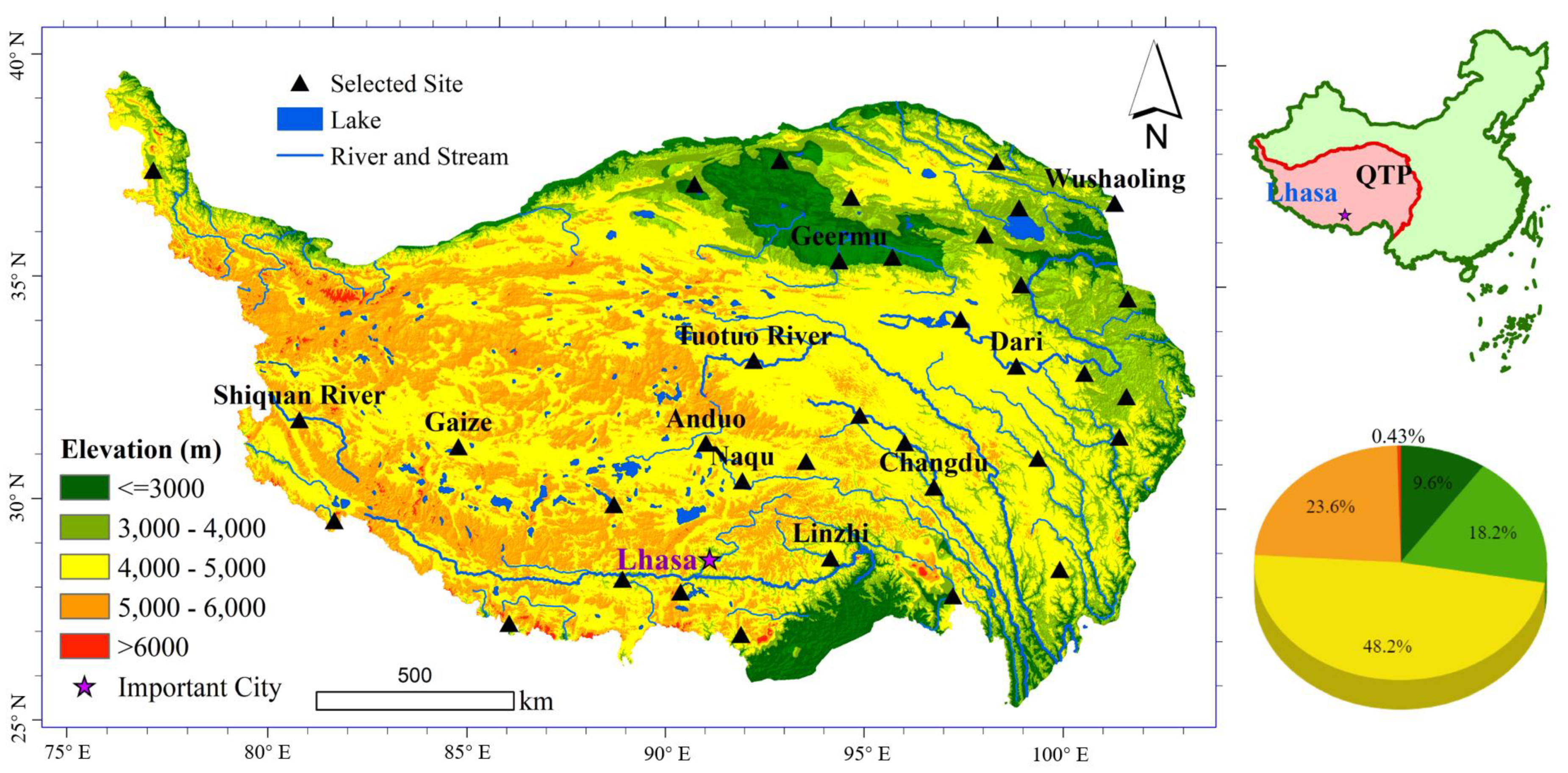
Map showing the location and topography of the Qinghai-Tibet Plateau (QTP) and the sites under investigation. The pie chart shows the proportions of different elevational zones on the QTP.
Atmosphere 12 01170 g001
Figure 2. Illustrations of the variables involved in the quantile–quantile (Q-Q) adjustment approach with an example of air temperature on the Naqu site, with the control period being 1970–1984 and projection period being 1985–1999. Left shows the probability density functions (PDF) and the right, the cumulative density functions (CDF). The notations used are consistent with those in Equations (1)–(6). The lines of calibrated future projection represent the results after the adjustment. The vertical straight lines in the PDF subplot represent the means of the observations ( O ¯ ) and raw simulations ( s c ¯ ) in the control period and the mean of the simulations in the projection period ( s f ¯ ). The percentile pairs used are the 25th and 75th and their corresponding values are described by Q ( 25 % ) and Q ( 75 % ) in the CDF subplot. Raw control simulation and raw future simulation data are from the GCM simulations; control observed data are the site observations or the calibrated results produced in the preceding adjustment; and calibrated future projection data are the results desired. The illustrative plot is created by the authors with reference to the concept of Yang et al. [78].
Atmosphere 12 01170 g002
Figure 3. Calibrated results (the ordinates) and corresponding monthly observations (the abscissas) of five major meteorological variables at the 36 QTP sites in the first adjustment (1970–1984 as the control period and 1985–1999 as the projection period). The color ramp in the figure symbolizes the kernel density. The red solid lines represent a 1:1 line. The orange dashed lines represent the linear fitting curves of the samples in the subplots with the R square of each variable marked. Subplots (a,c,e,g,i) show the results from EC-Earth 3 (EC) GCM simulations; and (b,d,f,h,j) the MPI-ESM1.2-HR (MPI) GCM simulations.
Atmosphere 12 01170 g003
Figure 4. Time series of the pre-adjustment GCM simulations, calibrated results, and the observations in the last adjustment (the results in the 2000–2014 period) for the variables at the Naqu site. Raw simulations: pre-adjustment data from the EC and MPI GCM simulations; calibrated results: post-adjustment results; validation: the corresponding observations in 2000–2014. Subplots (ae) correspond to precipitation, air temperature, relative humidity, wind speed and air pressure.
Atmosphere 12 01170 g004
Figure 5. Spatial distributions of the NMAE values of the calibrated results and the raw GCM simulations of atmospheric variables at the 36 selected QTP sites from two GCM data (middle: (b,e,h,k,n) for EC; right: (c,f,i,l,o) for MPI) for the first adjustment (results corresponding to 1985–1999), together with the 15-year means of the variables observed in the same period (left: (a,d,g,j,m)). Rows from the upper down represent precipitation (ac), air temperature (df), wind speed (gi), relative humidity (jl) and air pressure (mo), respectively. The NMAE values are broken into 5 classes. In the middle and right panels, the color of the circle represents the class of NMAE value of the raw GCM simulations (blue to red for low to high NMAE; annotated as Raw NMAE) and the size of the circle represents the magnitude of NMAE value of the calibrated results (small to large circles for low to high NMAE; annotated as Calibrated NMAE). N = 180 for each site.
Atmosphere 12 01170 g005
Figure 6. Calibrated results (the ordinates) and corresponding monthly observations (the abscissas) of five major meteorological variables at the 36 QTP sites in the second adjustment (2000–2014 as the projection period). The same notations as those applied in Figure 3. (a,c,e,g,i) show the results from EC GCM simulations; and (b,d,f,h,j) the MPI GCM simulations.
Atmosphere 12 01170 g006
Figure 7. Bar chart showing the changes in NMAE of the calibrated results of the first adjustment (1985–1999) using different pairs of percentiles at the sites of Naqu (a), Wushaoling (b) and Shiquan River (c). The left y-axis devotes to the MPI and the right y-axis to the EC data. The number appearing above or below a bar indicate the change in NMAE value of this percentile pair relative to the default pair ((10,90) for precipitation and (25,75) for the rest). The NMAE values for air pressure are all very close to zero, such that they are not clearly depicted. Note that extreme events were not excluded when processing precipitation. N = 180 on each site.
Atmosphere 12 01170 g007
Figure 8. Changes in PDF during the successive adjustments of air pressure based on the GCM MPI simulations at the Naqu site. The upper row indicates the control observations ((a), 1955–1969)) and the calibrated results of the three adjustments (bd). The center row (eg) indicates the observations for validating the calibrated results for the corresponding projection periods. The bottom row (hk) indicates the raw GCM simulations in the corresponding periods. The first column: control period (1955–1969); the second to fourth columns: the first (1970–1984), second (1985–1999) and third (2000–2014) adjustments, respectively. The solid line indicates a distribution fit to the data.
Atmosphere 12 01170 g008
Figure 9. Changes in PDF during the successive adjustments of precipitation based on the GCM MPI simulations at the Naqu site. Precipitation is displayed as an example of mismatching PDF between the observations and the GCM simulations. The upper row indicates the control observations ((a), 1955–1969)) and the calibrated results of the three adjustments (bd). The center row (eg) indicates the observations for validating the calibrated results for the corresponding projection periods. The bottom row (hk) indicates the raw GCM simulations in the corresponding periods. The first column: control period (1955–1969); the second to fourth columns: the first (1970–1984), second (1985–1999) and third (2000–2014) adjustments, respectively. The solid line indicates a distribution fit to the data.
Atmosphere 12 01170 g009
Figure 10. Changes in CDF of the five major variables during the successive adjustments at the Naqu site based on GCM MPI simulations. The abscissa is the value of the variable and the ordinate is the cumulative density. The left (a,d,g,j,m), middle (b,e,h,k,n) and right (c,f,i,l,o) columns represent the first (1970–1984), second (1985–1999) and third (2000–2014) adjustments, respectively. Rows from the upper down represent precipitation (ac), air temperature (df), relative humidity (gi), wind speed (jl) and air pressure (mo), respectively. Control observed and raw control: the site observations and the raw GCM simulations in the control period (1955–1969); future calibrated and raw future: the calibrated results and the raw GCM simulations in the projection period of the first adjustment (1970–1984); validation: the observations in 1970–1984 for validating the calibrated results. The closer the future calibrated and validation, the better the performance.
Atmosphere 12 01170 g010
Figure 11. Calibrated results (the ordinates) by the Q-M method and the corresponding monthly observations (the abscissae) of five major meteorological variables at the 36 QTP sites in the first adjustment (projection period being 1985–1999). The symbolic notations are the same as in Figure 3. Subplots (a,c,e,g,i) show the results from EC GCM simulations; and (b,d,f,h,j) those of the MPI GCM simulations.
Atmosphere 12 01170 g011
Figure 12. Calibrated results (the ordinates) by the delta downscaling method (Delta) and the corresponding monthly observations (the abscissae) of five major meteorological variables at the 36 QTP sites for the first adjustment (results corresponding to 1985–1999). The symbolic notations are the same as in Figure 3. Subplots (a,c,e,g,i) show the results from EC GCM simulations; and (b,d,f,h,j) the MPI GCM simulations.
Atmosphere 12 01170 g012
Table 1. Averaged performance of the Q-Q approach for monthly variables from EC-Earth 3 (EC) and MPI-ESM1.2-HR (MPI) GCM simulations over the 36 selected sites on the QTP against the site observations in terms of root mean square error (RMSE), mean absolute error (MAE) and normalized mean absolute error (NMAE). The results for the first and second adjustments refer to the calibrated results in the 1985–1999 and 2000–2014 periods, and the raw simulation refers to the uncalibrated GCM simulations in 1985–1999 as a reference before the adjustment. The second adjustment was made based on the results of the first adjustment. The units of RMSEs and MAEs are the same as those of the variables, while NMAE is dimensionless. N = 180 for each site.
VariableRaw SimulationFirst AdjustmentSecond Adjustment
RMSEMAENMAERMSEMAENMAERMSEMAENMAE
Relative humidity (%)EC28.9225.460.5310.658.370.1711.378.940.18
MPI35.1729.900.6311.018.770.1811.238.870.20
Precipitation (mm)EC46.3532.071.2943.0729.251.0557.0438.481.08
MPI47.6335.701.9239.4826.730.9256.6238.911.09
Air pressure (hPa)EC339.05338.920.543.032.380.003.132.470.00
MPI327.98327.900.523.782.990.003.492.760.00
Air temperature (°C)EC8.547.240.976.205.580.648.177.620.86
MPI7.366.160.843.182.430.327.847.010.81
Wind speed (m/s)EC1.571.310.531.591.250.511.681.320.54
MPI1.781.440.631.281.000.411.481.140.76
Table 2. Stats of Pearson’s correlation coefficient ( r ) at the 36 QTP sites before (Raw) and after (Calibrated) the first adjustment (1985–1999) based on two GCM simulations (EC and MPI). The coefficients are measured against the observations. The medians ahead the parentheses, and the minima and maxima within the parentheses. The upward and downward arrows indicate the gain and loss in r from the adjustment compared to the raw simulations. N = 180 for each site.
VariableGCM ECGCM MPI
RawCalibratedRawCalibrated
Relative humidity (%)−0.67(−0.82, 0.16)↑ 0.67(0.19, 0.85)−0.62(−0.78, 0.26)↑ 0.59(0.20, 0.79)
Precipitation (mm)0.16(−0.03, 0.28)↑ 0.38(0.04, 0.49)0.29(−0.18, 0.41)↑ 0.35(0.06, 0.43)
Air pressure (hPa)−0.41(−0.68, 0.58)↑ 0.64(0.29, 0.73)−0.22(−0.65, 0.63)↑ 0.58(0.22, 0.62)
Air temperature (°C)0.94(0.44, 0.97)↓ 0.93(0.90 ↑, 0.95)0.96(0.47, 0.96)↓ 0.88(0.84 ↑, 0.90)
Wind speed (m/s)−0.14(−0.28, 0.21)↑ 0.20(0.01, 0.35)−0.12(−0.40, 0.28)↑ 0.14(−0.07, 0.32)
Table 3. Performance of this adjustment approach averaged over the 36 QTP sites stratified by seasons in terms of RMSE and MAE values before (raw) and after (calibrated) the first adjustment based on the GCM EC data. The metrics are measured against the site observations. N = 45 on each site for each season.
VariableSpring (MAM)Summer (JJA)Autumn (SON)Winter (DJF)
RawCalibratedRawCalibratedRawCalibratedRawCalibrated
Relative humidity (%)RMSE28.0910.3129.1710.0222.3610.8231.2610.89
MAE24.758.1627.857.8619.298.7029.958.77
Precipitation (mm)RMSE26.8146.2475.1887.3139.5648.2913.7230.93
MAE20.4933.3866.2968.2130.1233.9811.3721.05
Air pressure (hPa)RMSE341.212.74329.261.94337.332.67348.074.19
MAE341.132.20329.251.63337.282.26348.023.41
Air temperature (°C)RMSE8.086.197.485.606.195.9710.406.83
MAE6.865.627.135.235.285.469.706.02
Wind speed (m/s)RMSE1.811.741.391.101.401.461.531.89
MAE1.561.361.220.891.181.191.271.55
Table 4. Changes of RMSE and MAE values at the Naqu site as the adjustment proceeds and the adjustment window varies. Raw simulation and the first adjustment refer to the raw GCM simulations and the calibrated results in 1970–1984, the second adjustment, 1985–1999 and the third adjustment, 2000–2014. The next adjustment depends on the calibrated results in the preceding adjustment as control or the observations in 1955–1969 as the initial control (for the first adjustment). The metrics are measured against the site observations. The column titled 30-year window is the calibrated results in 1985–2014 using a 30-year adjustment window, which temporally contains the second and third adjustments using 15-year window. N = 180 for the 15-year time window and N = 360 for the 30-year time window.
VariableRaw SimulationFirst AdjustmentSecond AdjustmentThird Adjustment30-Year Window
RMSEMAERMSEMAERMSEMAERMSEMAERMSEMAE
Relative humidity (%)EC28.7625.5215.9812.5917.8614.6417.6214.4718.1614.98
MPI35.1028.6218.0814.5220.0716.0419.4415.3617.6414.15
Precipitation (mm)EC48.0332.0452.0035.0556.9039.0274.2450.2351.4334.12
MPI44.5933.4944.2429.1357.9639.5362.1645.0744.2628.84
Air pressure (hPa)EC420.42420.302.641.822.802.062.762.032.611.94
MPI409.35409.283.202.424.273.014.032.833.472.53
Air temperature (°C)EC7.736.803.312.544.884.066.875.955.384.61
MPI7.646.413.662.664.613.314.743.563.672.79
Wind speed (m/s)EC1.411.121.190.942.201.732.501.981.741.33
MPI1.531.191.220.942.011.462.561.991.481.14
Table 5. RMSE and MAE values before and after the removal of daily precipitation extremes in the control observations at three different sites.
SiteVariableBefore Removing ExtremesAfter Removing Extremes
ECMPIECMPI
NaquRMSE (mm)52.0044.2446.1642.56
MAE (mm)35.0529.1329.8728.14
WushaolingRMSE (mm)49.8841.8238.6036.66
MAE (mm)34.0528.0926.6224.77
Shiquan RiverRMSE (mm)18.0717.9613.0013.20
MAE (mm)11.0110.686.046.04
Table 6. Comparison in adjusting air temperature by using fitted values of the g parameter over the original form of g (Equation (5)) in terms of RMSE at five representative sites. The control and projection periods correspond to 1970–1984 and 1985–1999, respectively. The GCM MPI is used. s c ¯ is the average air temperature in the control period on the site. Q-M stands for the quantile mapping method.
Site
( s c ¯ ,   ° C )
Q-Q Using Original gQ-Q Using Fitted gQ-M
RMSE (°C)gRMSE (°C)gRMSE (°C)
Naqu
(2.39)
3.02−0.122.191.082.92
Gaize
(3.20)
3.600.963.600.893.11
Geermu
(3.65)
3.591.023.150.783.21
Langkazi
(0.23)
7.5012.563.710.666.29
Maduo
(0.94)
3.58−4.393.980.763.50
Table 7. Comparison of performance of the three comparative adjustment methods in terms of mean RMSE and MAE over the 36 QTP sites after the first adjustment (1985–1999) based on two GCM simulations (EC and MPI). N = 180 for each site.
VariableThis ApproachQ-M MethodDelta Method
RMSEMAERMSEMAERMSEMAE
Relative humidity (%)EC10.658.3720.6918.0325.2822.32
MPI11.018.7720.2617.8226.6823.86
Precipitation (mm)EC43.0729.2544.7430.6141.8029.29
MPI39.4826.7342.7329.3140.4128.10
Air pressure (hPa)EC3.032.384.203.578.917.63
MPI3.782.994.713.947.326.06
Temperature (°C)EC6.205.582.602.037.796.64
MPI3.182.433.022.276.675.57
Wind speed (m/s)EC1.591.251.371.081.571.24
MPI1.281.001.170.941.511.19
Publisher’s Note: MDPI stays neutral with regard to jurisdictional claims in published maps and institutional affiliations.

