Abstract
A comparison was made of two eddy dissipation rate (EDR) estimates based on flight data recorded by commercial flights. The EDR estimates from real-time data using the National Center for Atmospheric Research (NCAR) Algorithm were compared with the EDR estimates derived using the Netherlands Aerospace Centre (NLR) Algorithm using quick assess recorder (QAR) data. The estimates were found to be in good agreement in general, although subtle differences were found. The agreement between the two algorithms was better when the flight was above 10,000 ft. The EDR estimates from the two algorithms were also compared with the vertical acceleration experienced by the aircraft. Both EDR estimates showed good correlation with the vertical acceleration and would effectively capture the turbulence subjectively experienced by pilots.
1. Introduction
Turbulence is a hazardous weather phenomenon and is the main cause of weather-related reported aircraft incidents and accidents [1]. The impact of the turbulence depends on the eddy magnitude and size, aircraft type specific parameters (such as weight, wing span, airspeed, etc.), and the phase of the flight during which the turbulence occurs. Although there are a wide range of eddy sizes in the atmosphere, aircraft mainly respond to eddies having sizes in the order of tens to hundreds of meters. Eddies of this size can be created by an energy cascade [2], i.e., a larger eddy in the atmosphere breaks up and forms a smaller eddy, which eventually dissipates as heat.
Forecasting turbulence is of great interest for scientific research. A number of Numerical Weather Prediction (NWP)-based turbulence forecast techniques have been developed in recent decades [3,4,5]. Because the scale of interest for turbulence forecasting is in the order of hundreds of meters, which is outside the current scope of state-of-the-art operational NWP, these turbulence forecasts are often still diagnostic based, i.e., forecasting the weather quantities that are prone to create an eddy of the right size to result in an impact with an aircraft [5]. As a result, parameters in these forecast techniques often need to be “calibrated” using turbulence observations.
Observations of turbulence fall into two categories, i.e., subjective and objective observations. Subjective observations mainly take the form of pilot reports. Although turbulence experienced by the pilot must be of the right eddy size to result in impact, such observations are highly aircraft-type dependent. As aircraft response decreases with wing loading and increases with altitude and airspeed [1,6], the same atmospheric eddy can result in a drastically different impact for different aircraft. The same atmospheric eddy may be reported as causing severe turbulence by pilots of smaller aircraft, whereas pilots of large aircrafts would barely feel its effect. A previous study found that pilot reports are considered inadequate for observing turbulence if used alone [7].
Turbulence can also be measured objectively, independent of the aircraft type, in turbulence metrics such as the cubic root of the eddy dissipation rate (EDR) [8] and derived equivalent vertical gust velocity (DEVG) [9,10,11,12]. Both ICAO and WMO adopted EDR as the official turbulence reporting metric. Two notable EDR estimation algorithms exist in the literature, i.e., the algorithm developed by the National Aerospace Laboratory (NLR) in the Netherlands (the NLR Algorithm), which can estimate EDR using data recorded in the quick assess recorder (QAR) [13], and the algorithm developed by NCAR (the NCAR Algorithm) [14,15], which was adopted by Boeing and is implemented on Boeing aircraft.
Although both algorithms estimate the EDR from estimates of the vertical component of wind in the flight data, differences exist in the underlining assumptions of the two algorithms. Differences in the EDR estimates, if any, can easily be misinterpreted as differences in the turbulence climatology of geographical regions due to differences in the spatial coverage of the data. The NCAR Algorithm provides a more global coverage of the EDR estimates because it is implemented in the onboard software of Boeing aircraft in a number of large airlines, and the EDR data can be shared among airlines through the IATA Turbulence Aware Program. By comparison, the EDR estimates from the NLR Algorithm are more local because the algorithm is applied on flight data recorded in the QAR, which is more dependent on the operating region of the airline. The difference in the EDR estimates can also lead to sub-optimal tuning of parameters in NWP turbulence forecasts, which can impact the confidence of the users in the forecast products.
This article compares the estimated EDR values between the two algorithms. The article is organized as follows: Section 2 provides a brief description of the two algorithms; the comparison results are shown in Section 3, with highlights of the differences between the two EDR estimates, followed by a discussion of the results in Section 4. The article is summarized in Section 5.
2. Methods and Data Sets
Although both NCAR and NLR Algorithms estimate the EDR from the wind, there are subtle differences between the two methods. The differences are discussed below.
2.1. Brief Description of the NLR Algorithm
The NLR Algorithm is a wind-based algorithm that calculates the EDR () using:
where is a low-pass filtered airspeed that represents the average flying speed, and is the running standard deviation of the band-pass-filtered vertical wind variations computed with cut-off frequencies and , which correspond to 0.1 and 2 Hz in this study. The sliding window has a length of 10 s. It is noted that the aircraft QAR does not directly record wind data and that the wind is a minimum variance estimate from the data available in the QAR. The vector of the wind data , and hence the vertical component of the wind, is estimated by:
where the inertial speed vector is in the Earth reference frame and is estimated by the ground speed and track angle. The aerodynamic speed vector is estimated by aerodynamic speed, angle of attack, and sideslip angle, and is originally calculated in the aircraft body reference frame, which needs to be transformed back to the Earth reference frame using Euler angles. Interested readers should refer to [13] for details.
2.2. Brief Description of the NCAR Algorithm
The NCAR Algorithm is a vertical wind-based algorithm that calculates the EDR () using:
where the summation is done over the frequency domain with frequencies, is the power spectrum of the vertical wind component, is the bias-correction term, and is a reference model spectrum in which the von Karman spectral model valid for an incompressible isotropic turbulent velocity field is used. The vertical wind component is estimated in a manner similar to that shown in Equation (2) except that the sideslip angle is assumed to be 0. The NCAR Algorithm is implemented by Boeing on the B777 aircraft and the authors do not have access to the details of the implementation.
The functional forms of both NCAR and NLR Algorithms match well in terms of their dependence on the vertical wind speed. However, the reference model spectrum and the assumption regarding the sideslip angle differ, and are potentially some of the sources of the differences observed in the comparison study below.
2.3. Vertical Acceleration Experienced by the Aircraft
Because pilots report the severity of turbulence based on their subjective feeling of the degree of shaking during a flight, we also examined the vertical acceleration recorded by the QAR to see how well it correlates with the EDR estimates. In this study, the root-mean-square of Acceleration (RMS-g) was computed from the B777 vertical acceleration recorded in a 10 Hz data frequency. To avoid underestimating the severity of short events while reducing the variations in the calculation, a running 5 s averaging window was used in the computation of RMS-g [16].
2.4. Data Sets in the Comparison Study
The NCAR Algorithm runs on the onboard computer of the B777 fleet of Cathay Pacific and outputs through a real-time data downlink. There is thus a trade-off between data volume and data representativeness. In the current implementation, the NCAR Algorithm outputs, at most, every minute for its 1 min mean and peak EDR estimates from its internal data. Regarding the NLR Algorithm, because the software we use runs in a post-analysis mode, there is no limitation due to the bandwidth of the real-time data downlink and the software outputs its EDR estimates in a 4 Hz data frequency. For any particular flight, significantly more data exists from the NLR Algorithm than from the NCAR Algorithm. To match the output data for the two algorithms on the flights, we down-sampled the output from the NLR Algorithm. For each datapoint from the NCAR Algorithm, we computed the past 1 min peak EDR estimates from the NLR Algorithm of the same time. The peak EDR estimates were used, due to their higher sensitivity, to highlight any discrepancy between the two algorithms. For the vertical acceleration, the past 1 min peak RMS-g was computed from the 10 Hz vertical acceleration data recorded by the B777 over the same time period.
3. Results
The NCAR Algorithm has been implemented on the B777 fleets of Cathay Pacific since early 2020 [17], and we had access to all EDR estimates from the NCAR Algorithm from Cathay Pacific B777 flights in real time. The EDR estimates from the NLR Algorithm were obtained via a specific request to Cathay Pacific for the provision of QAR data from particular flights. The EDR estimates were then computed from those QAR data. Because a significant proportion of the flights are uneventful (EDR < 0.2 from the NCAR Algorithm throughout the whole flight, referred to as “smooth flights” in the following text), we only requested QAR data of flights with at least one EDR estimate ≥0.2 in the period from April 2020 to June 2021 for this comparison study, i.e., flights that experienced at least moderate turbulence according to the ICAO definition. Due to the significant reduction in the number of flights due to travel restriction as a result of the COVID-19 pandemic, only 107 flights met this criterion and were included in this study. For these 107 flights that experienced moderate turbulence during a portion of their flights, data from the non-turbulent portion of the flight were also included in this study, and these non-turbulent data still represented the majority of data in the dataset.
3.1. Spatial Distribution of Flight Data
The spatial distribution of the flight data from the 107 flights is shown in Figure 1. There are a total of 5739 datapoints in the comparison. Most of the data are located in the Asia-Pacific region, which is due to the operational characteristics of Cathay Pacific. The dataset showed four areas where turbulence is more prominent, i.e., (1) over the western part of North Pacific, (2) over eastern China, (3) near Himalaya, and (4) over the equatorial region. The first three areas agree well with previous studies in the literature [18].
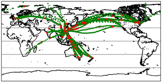
Figure 1.
Spatial distribution of the flight data used in the comparison. Green dots are for flight datapoints with estimated EDR < 0.2 by the NCAR Algorithm, whereas red dots are for those with estimated EDR ≥ 0.2.
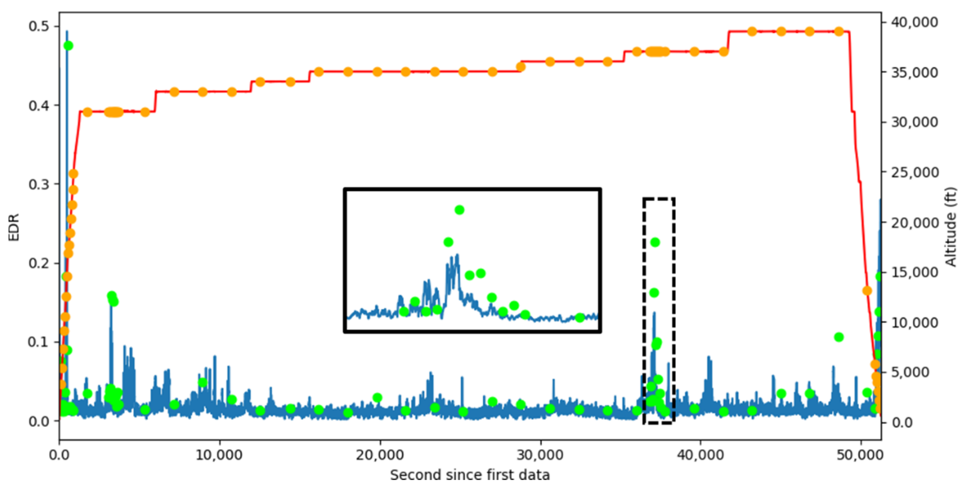
3.2. Examples of EDR Time Series from NLR and NCAR Algorithms
An example of EDR estimates from the two algorithms is shown in Figure 2. The actual time of the EDR estimates is not shown for a particular flight for confidentiality reasons. Instead, both the altitude of the flight and the EDR estimates from the two data sources are shown in Figure 2 to demonstrate the close match of the two EDR estimates. The EDR estimates from the NLR Algorithm are plotted in its full resolution of 4 Hz. Thus, the figure shows the short-term fluctuation in the EDR estimates that cannot be observed in the EDR estimates from the NCAR Algorithm due to its limited temporal resolution.
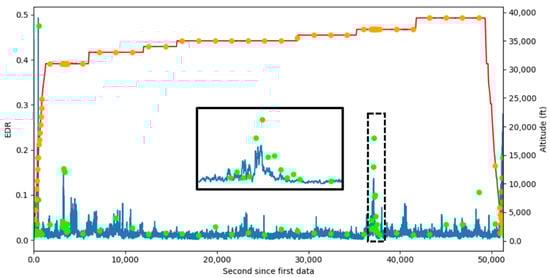
Figure 2.
An example time series of the EDR estimates from the two algorithms. Data from the NCAR Algorithm is shown in dots, whereas the data from the NLR Algorithm is shown in lines. EDR estimates are in lime and blue. The altitude of the data from the two data sources (red and orange) are also shown in the figure to validate a correct matching between the two data sources. The insert shows the magnification of the data inside the dashed black rectangle.
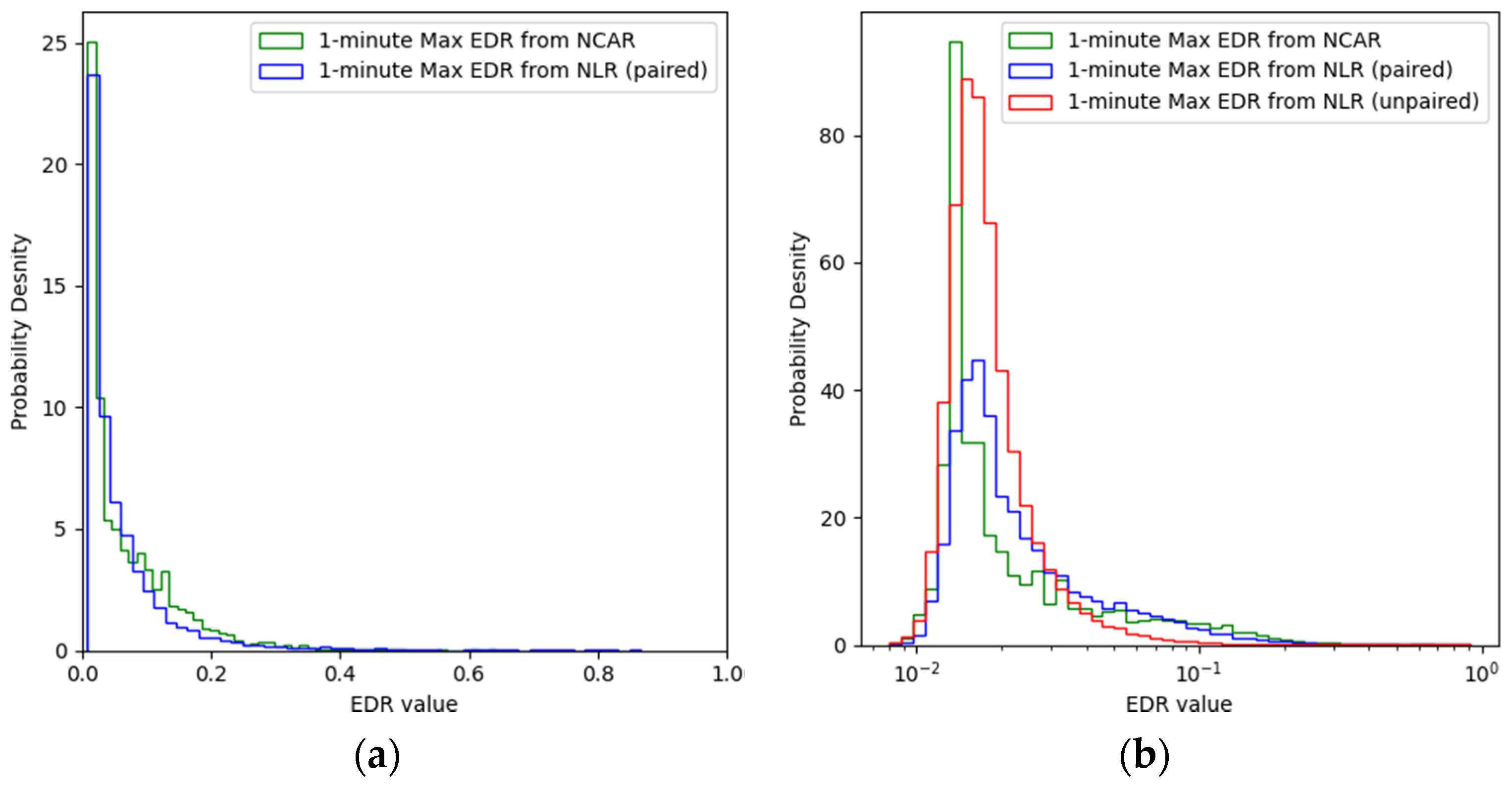
3.3. Frequency Distribution of EDR Estimates
The frequency distribution of the estimated values of the EDR is shown in Figure 3. It is noted that the frequency distribution shown in Figure 3 does not resemble the actual climatology of EDR in the atmosphere due to three reasons: (1) the EDR is only sampled along flight routes; (2) smooth flights are excluded in the dataset; and (3) the onboard software of the B777, which uses the NCAR Algorithm, outputs EDR with a variable frequency depending on the estimated EDR, i.e., during a more turbulent flight, the onboard software outputs and reports the EDR every minute, whereas during non-turbulent flight, the frequency of output is reduced to every 15 min. Although the exact criteria for the change in the reporting frequency is not known to the authors, examples of strategies for the triggering of the change in the reporting frequency are discussed in [15]. Because of the latter two reasons noted above, the sampling is inherently biased towards higher EDR. Because we paired the estimates from the NLR Algorithm with those from the NCAR Algorithm for this comparison study, the frequency distribution of the EDR estimates from the NLR Algorithm shown in Figure 3 is also biased in the same manner.
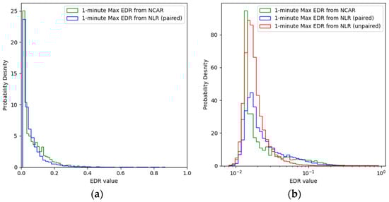
Figure 3.
The frequency distribution of the EDR data computed from the two algorithms. (a) The frequency distribution over the full range of EDR. (b) The same as (a), except that the horizontal axis is in log scale. The frequency distribution of all EDR estimates (without pairing with the reporting frequency of the EDR from the NCAR Algorithm) is shown in red.
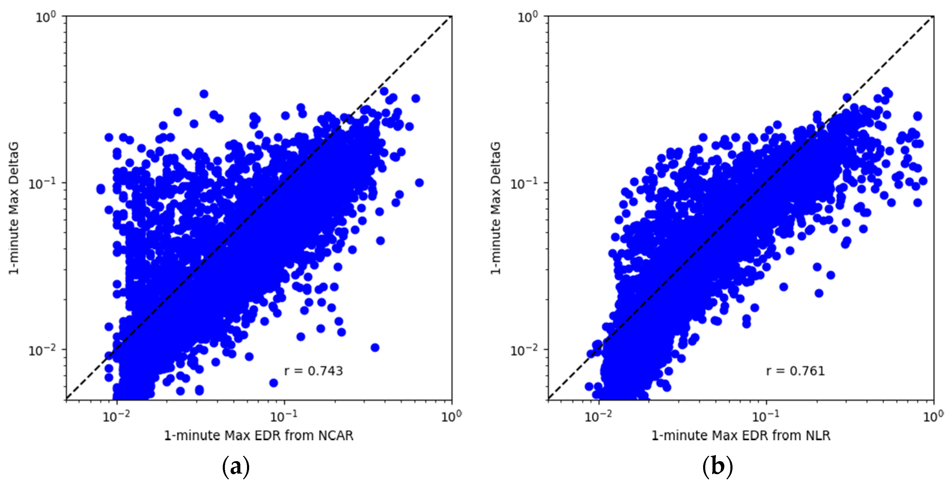
3.4. Comparisons between the EDR Estimates from the Two Algorithms
A scatter plot showing the comparison between the two algorithms is shown in Figure 4. To allow a closer look at the data, the data pairs are further partitioned based on the altitude and latitude of the data. It would be of significant interest to study if there are observable differences in the EDR estimates for the two algorithms for turbulence resulting from different sources, i.e., convection, jet stream, mountain wave, etc., due to the differences in the assumptions of the two algorithms. Ideally, such partitioning of data would be best accomplished by examining the onboard radar data and/or satellite pictures with high temporal resolution at the time. However, because this data was not available to us, an alternative simplified approach was taken in this study, i.e., partitioning the data based on their latitude. For datapoints located in the tropical region (between 30° S and 30° N), it is inferred that the main source of turbulence was convection, because most of the turbulence events are recorded close to the equator, as shown in Figure 1, whereas for datapoints in the extratropical region, the source was mixed. The data is also partitioned to isolate those captured at low levels (no greater than 10,000 ft in altitude). This is to also study if the two algorithms differ in estimating the EDR for low level terrain-induced turbulence, as those low-level data are captured during takeoff or landing of the aircraft. Because most of the Cathay Pacific flights are either taking off from or landing at the HKIA, the low-level data around HKIA are also plotted to study if the local environment at HKIA has any significant impact on the comparison. The results of this partitioning are shown in Figure 5.
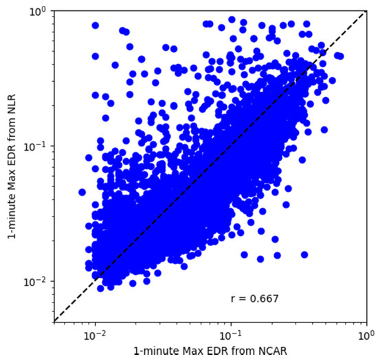
Figure 4.
Scatter plot comparing the EDR computed from the two algorithms. Although there are outliners in both algorithms, the EDR values from the two algorithms agree well.
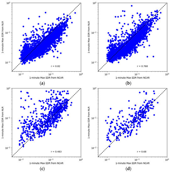
Figure 5.
A closer examine of the results shown in Figure 4 by partitioning of the data: (a) results for mid to upper levels over extratropical and polar regions (north of 30° N or south of 30° S, and over 10,000 ft in altitude); (b) results for the tropical region (between 30° N and 30° S, and over 10,000 ft in altitude); (c) results for EDR estimates at low levels (no greater than 10,000 ft in altitude); and (d) results for EDR estimates around Hong Kong International Airport.
3.5. Comparisons of the EDR Estimates with RMS-g
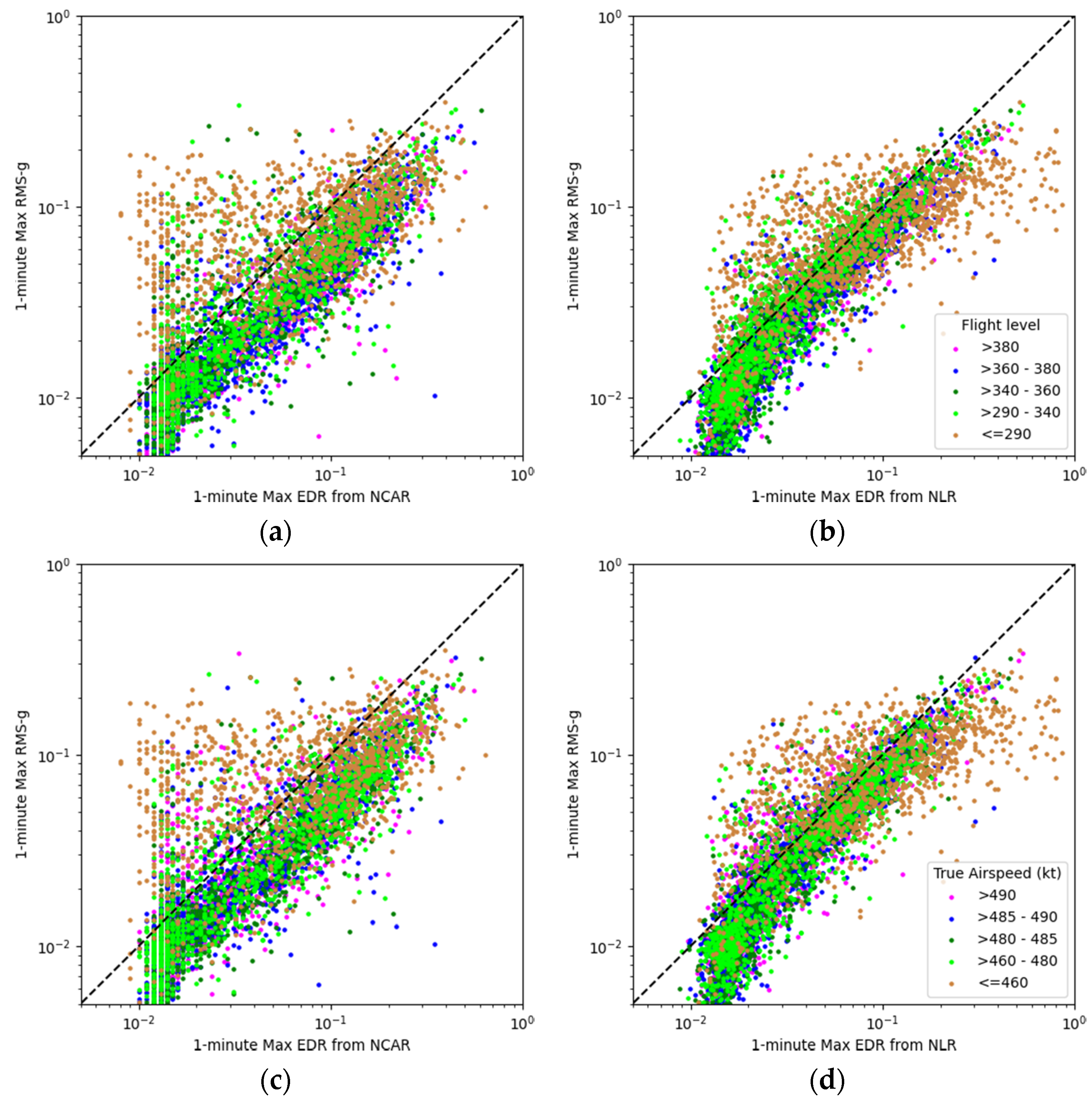
The scatter plots showing the comparisons between the EDR estimates and the RMS-g are shown in Figure 6. In theory, the relation between RMS-g and EDR should depend on airspeed and altitude. To see the dependence on these variables, the dataset was partitioned according to the altitude or true airspeed. The results of the partitioning are shown in Figure 7. The class boundaries of the partitioning were chosen so that each data category contained around 1/5 of the data of the whole dataset.
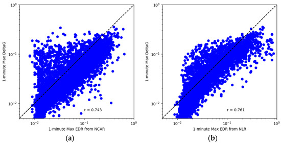
Figure 6.
Comparisons between the NCAR EDR estimates (a) and the NLR EDR estimates (b) with RMS-g recorded in the QAR data.
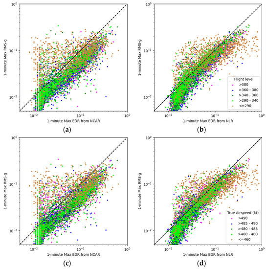
Figure 7.
Same as Figure 6, except the data is partitioned according to: (a,b) altitude t; and (c,d) true air speed. Comparisons between the NCAR EDR estimates with RMS-g are shown on the left (a,c), whereas the comparisons between the NLR EDR estimates with RMS-g are shown on the right (b,d).
4. Discussion
Figure 3 shows a close match in terms of the frequency distribution of the EDR estimates. Compared with the frequency distribution of the EDR estimates from the NCAR Algorithm, the frequency distribution of the EDR estimates from the NLR Algorithm is slightly biased to the right. However, this bias is inconsequential for the reporting of turbulence from the pilots because the turbulence severity at which this bias exists is well below the threshold for reporting any significant turbulence. There is also a slight excess in the relative frequency, compared with the NLR EDR, for the NCAR EDR estimates for EDR values around 0.1, and the origin of this excess is yet to be determined.
The frequency distribution of EDR in the atmosphere is expected to follow a log-normal distribution [15]:
However, the frequency distributions of EDR estimates from both of the algorithms shown in Figure 3b are positively skewed, whereas they are expected to be normally distributed when plotted in log scale for the horizontal axis. Hence, both EDR estimates in our dataset do not fit well to Equation (4). The derivation from the normal distribution is expected due to the bias towards higher EDR estimates caused by the sampling and reporting strategy, i.e., the inclusion of only turbulent flights in the study and the enhanced EDR reporting frequency for the NCAR Algorithm when the flight encountered turbulence. The values of and estimated by fitting the data to Equation (4) using Powell’s method are −3.59(−3.41) and 1.11(0.90), respectively, for the NCAR(NLR) algorithm, and are roughly comparable with those in [15].
The scatter plot in Figure 4 shows a good correlation between the two EDR estimates. By partitioning the EDR estimates according to the altitude and locations as shown in Figure 5, it was found that most of the disagreements between the two EDR estimates are recorded at lower altitudes (below 10,000 ft). The mean and root-mean-squared differences between the two EDR estimates for the lower altitude were found to be 0.073 and 0.140, respectively, compared with 0.031 and 0.063 for the whole dataset. For the EDR estimates in the middle and high altitude (above 10,000 ft) shown in Figure 5a,b, the distribution of the points is approximately symmetric over the diagonal line.
In addition, the scatter plots shown in Figure 5a,b closely resemble each other. The z score for testing the statistical significance for differences in the correlation is given by:
where and are the correlation and sample size of the two samples, respectively. This value was 5.10 (corresponding to a p-value of in a two-tailed test) when applied to testing the difference in the correlation shown in these two figures. However, if we limit the dataset and include only those data captured during turbulence (estimated EDR ≥0.1 from both algorithms), the corresponding z score drops to around 0.23 (corresponding to a p-value of 0.82 in a two-tailed test) because the sample size drops to almost of that of the original. The current differences in the correlation between the two algorithms mainly result from those small values of EDR estimates.
For EDR estimates of low levels (≤10,000 ft in altitude), it is clear from Figure 5c that the NLR Algorithm often estimates a higher EDR than the NCAR Algorithm. The same observations can also be deduced from Figure 5d, which focus on a single airport (Hong Kong International Airport). These low-level data are recorded during the ascent or descent of the flight. Aircraft usually operate in different settings when ascending or descending, i.e., with a higher flap and more frequent active maneuvering associated with pitching and rolling of the aircraft, than during en route flight. This difference in the aircraft operation settings may be attributed to the greater difference between the two EDR estimates at low levels. However, there are also only a limited number of flights included in this study, and no low-level en route flight is included in the dataset; hence, it is not possible to pinpoint the source of these differences.
The EDR estimates from both algorithms show similar correlations with the RMS-g (Figure 6) for the datasets as a whole, and the dependence of their correlations with the airspeed and altitude. For the data shown in Figure 7, among the five airspeed/altitude categories, the lowest one contains flight data recorded during the ascending and descending portion of the flight. It is in this data category that both EDR estimates showed the weakest correlation between the EDR estimates and the RMS-g, due to the larger variation in airspeed/altitude within this category of data. Although the relationship between the EDR, airspeed, altitude, and RMS-g is non-linear, if a multiple linear model is fitted for either EDR estimate + airspeed, or EDR estimate + altitude, against RMS-g, the coefficients of the linear model for the predictors would be similar if we compared the models fitted with NCAR and NLR EDR estimates. The fitted linear models would also suggest an increase in the RMS-g with an increase in airspeed or altitude, matching the theoretical prediction. It is not possible to fit a linear model using each of the three variables of EDR estimate, airspeed, and altitude as the predictors due to the strong correlation between airspeed and altitude.
5. Conclusions
In this study, we compared the EDR estimates from the NLR and NCAR Algorithms. In general, the EDR estimates from the two algorithms showed a good match with each other. However, the correlation of the two EDR estimates showed a dependence on both altitude and location. A further study with a larger dataset is required to pinpoint the source of these differences. A larger dataset can also allow for further partitioning of the dataset.
The NLR Algorithm is also used for estimating the EDR from QAR data recorded by other aircraft types, such as the Airbus A320 and A330. Because these aircraft usually fly shorter routes than the B777, the coverage of the EDR estimates from these aircraft would be different from those from the B777. Thus, differences between the two algorithms should be considered before pooling the EDR estimates for analysis, especially for analyzing low-level turbulence where the differences between the two algorithms is the greatest.
Author Contributions
Conceptualization, methodology, software, writing—original draft preparation, J.C.W.L.; Methodology, C.Y.Y.L.; Data acquisition and processing, communication with data provider, M.H.K.; Writing—review and editing, P.W.C. All authors have read and agreed to the published version of the manuscript.
Funding
This research received no external funding.
Institutional Review Board Statement
Not applicable.
Informed Consent Statement
Not applicable.
Data Availability Statement
Restrictions apply to the availability of these data. Data was obtained from the Boeing 777-300 and Boeing 777-300ER fleets of the Cathay Pacific Airways Ltd., Hong Kong, China and the authors are not authorized to share the data without the permission of Cathay Pacific Airways Ltd.
Acknowledgments
The authors would like to thank Cathay Pacific Airways Ltd. for the provision of the QAR data and EDR data for the study.
Conflicts of Interest
The authors declare no conflict of interest.
References
- Sharman, R. Nature of Turbulence. In Aviation Turbulence Processes, Detection, Prediction; Springer International Publishing: Cham, Switzerland, 2016; pp. 3–30. [Google Scholar]
- Kolmogorov, A.N. The local structure of turbulence in incompressible viscous fluid for very large Reynolds numbers. Proc. USSR Acad. Sci. 1941, 30, 299–303. [Google Scholar]
- Sharman, R.; Tebaldi, C.; Wiener, G.; Wolff, J. An integrated approach to mid- and upper-level turbulence forecasting. Weather Forecast. 2006, 21, 268–297. [Google Scholar] [CrossRef]
- Kim, J.H.; Chun, H.Y.; Sharman, R.; Keller, T.L. Evaluations of upper-level turbulence diagnostics performance using the Graphical Turbulence Guidance (GTG) system and pilot reports (PIREPs) over East Asia. J. Appl. Meteorol. Climatol. 2011, 50, 1936–1951. [Google Scholar] [CrossRef]
- Ellrod, G.P.; Knapp, D.L. An objective clear-air-turbulence forecasting techniques: Verification and operational use. Weather Forecast. 1992, 7, 150–165. [Google Scholar] [CrossRef] [Green Version]
- Hoblit, F.M. Gust Loads on Aircraft: Concepts and Applications; AIAA Education Series; American Institute of Aeronautics and Astronautics: Washington, DC, USA, 1988. [Google Scholar]
- Schwartz, B. The Quantitative Use of PIREPs in Developing Aviation Weather Guidance Products. Weather Forecast. 1996, 11, 372–384. [Google Scholar] [CrossRef] [Green Version]
- MacCready, P.B., Jr. Standardization of gustiness values from aircraft. J. Appl. Meteor. 1964, 3, 439–449. [Google Scholar] [CrossRef] [Green Version]
- Sherman, D.J. The Australian Implementation of AMDAR/ACARS and the Use of Derived Equivalent Gust Velocity as a Turbulence Indicator; Aeronautical Research Laboratorues Structures Rep.; Defense Technical Information Center: Fort Belvoir, VA, USA, 1985; Volume 418, p. 28. [Google Scholar]
- Truscott, B.S. EUMETNET AMDAR AAA AMDAR Software Development 2000; Technical Specification. Doc. Ref. E_AMDAR/TSC/003. Available online: ftp://ftp.wmo.int/Documents/www/amdar/standards/Final%20AAA%20Spec%202.pdf (accessed on 23 March 2021).
- Kim, S.H.; Chun, H.Y. Aviation turbulence encounters detected from aircraft observations: Spatiotemporal characteristics and application to Korean Aviation Turbulence Guidance. Meteorol. Appl. 2016, 23, 594–604. [Google Scholar] [CrossRef]
- Kim, S.H.; Chun, H.Y.; Chan, P.W. Comparison of Turbulence Indicators Obtained from In Situ Flight Data. J. Appl. Meteorol. Climatol. 2017, 56, 1609–1623. [Google Scholar] [CrossRef]
- Haverdings, H.; Chan, P.W. Quick Access Recorder Data Analysis Software for Windshear Turbulence Studies. J. Aircr. 2010, 47, 1443–1447. [Google Scholar] [CrossRef]
- Cornman, L.B.; Morse, C.S.; Cunning, G. Real-Time Estimation of Atmospheric Turbulence Severity from In-Situ Aircraft Measurements. J. Aircr. 1995, 32, 171–177. [Google Scholar] [CrossRef]
- Sharman, R.D.; Cornman, L.B.; Meymaris, G.; Pearson, J.; Farrar, T. Description and Derived Climatologies of Automated In Situ Eddy-Dissipation-Rate Reports of Atmospheric Turbulence. J. Appl. Meteorol. Climatol. 2014, 53, 1416–1432. [Google Scholar] [CrossRef]
- Emanuel, M.J.; Meymaris, G.; Cornman, L.; Sherry, J.; Mulally, D. EDR/RMS-G Correlation Analysis. In Proceedings of the American Meteorological Society (AMS) 98th Annual Meeting, Austin, TX, USA, 7–11 January 2018. [Google Scholar]
- Cathay Pacific Airways Limited; Hong Kong, China. Personal Communication, 2020.
- Jaeger, E.B.; Sprenger, M. A Northern Hemispheric Climatology of indices for clear air turbulence in the tropopause region derived from ERA40 reanalysis data. J. Geophys. Res. 2007, 112, D20106. [Google Scholar] [CrossRef] [Green Version]


Publisher’s Note: MDPI stays neutral with regard to jurisdictional claims in published maps and institutional affiliations. |
© 2022 by the authors. Licensee MDPI, Basel, Switzerland. This article is an open access article distributed under the terms and conditions of the Creative Commons Attribution (CC BY) license (https://creativecommons.org/licenses/by/4.0/).