
Multiscale Interactive Processes Underlying the Heavy Rainstorm Associated with a Landfalling Atmospheric River

Abstract
:1. Introduction
2. Data and Methodology
2.1. Data
2.2. Localized Multiscale Energetics Analysis
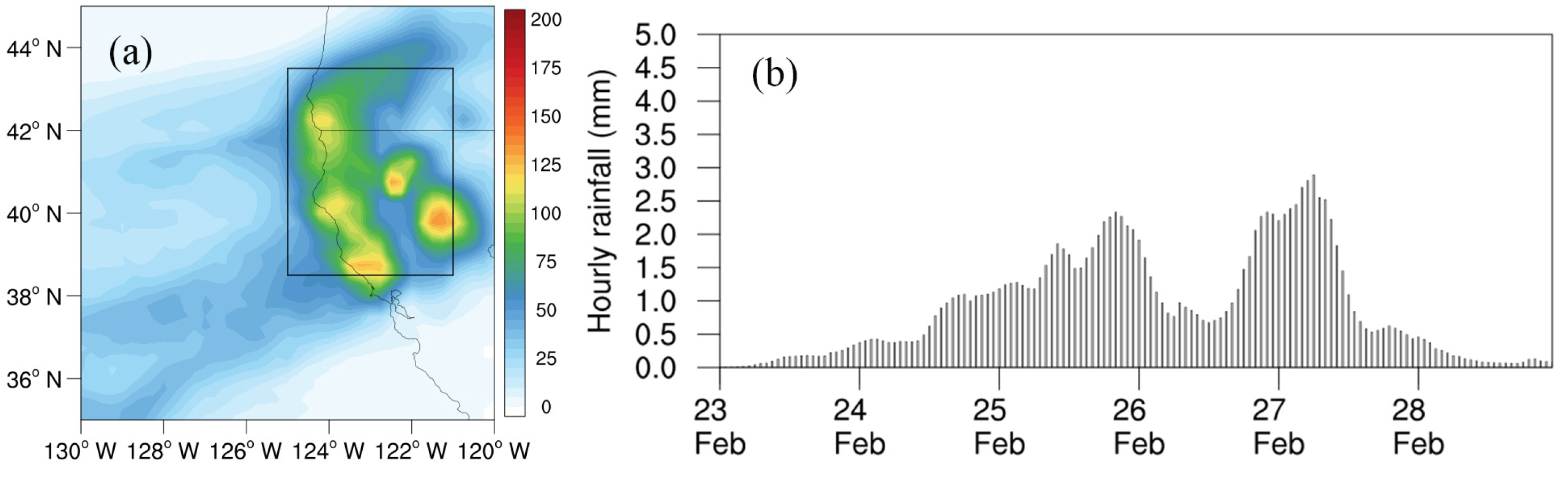
3. Characteristics of the Heavy Rainfall
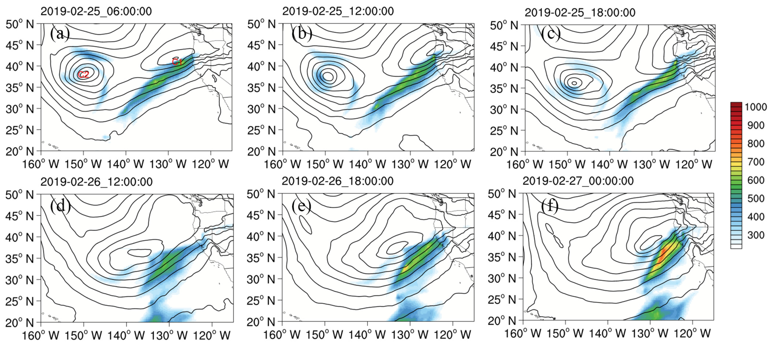
4. Scale Decomposition
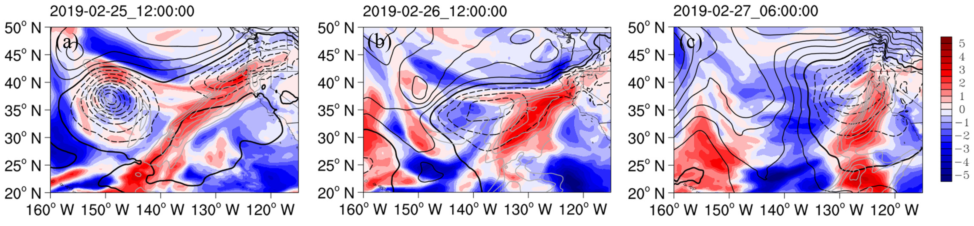
5. Dynamics Underlying the Extreme Precipitation
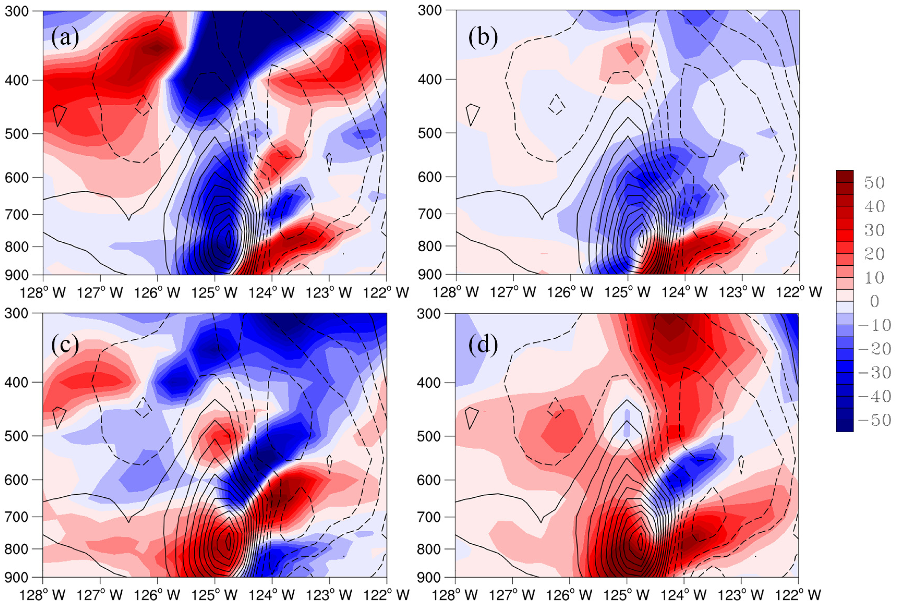
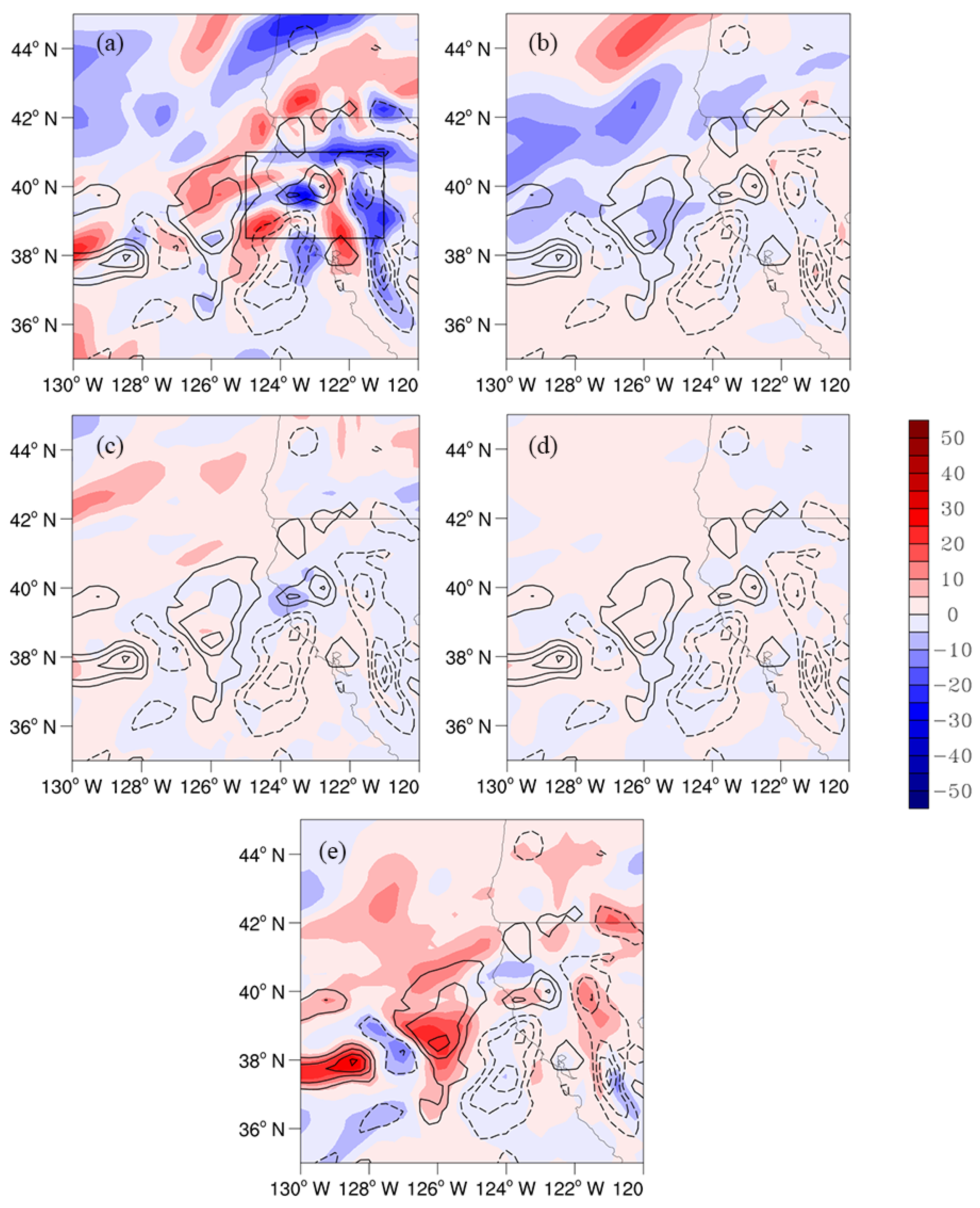
5.1. Stage I
5.2. Stage II
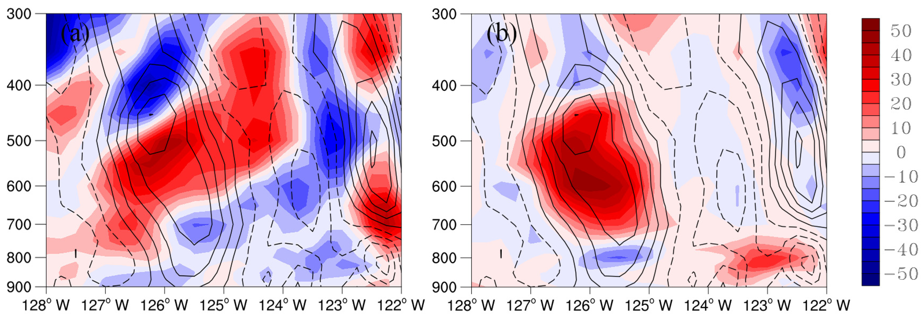
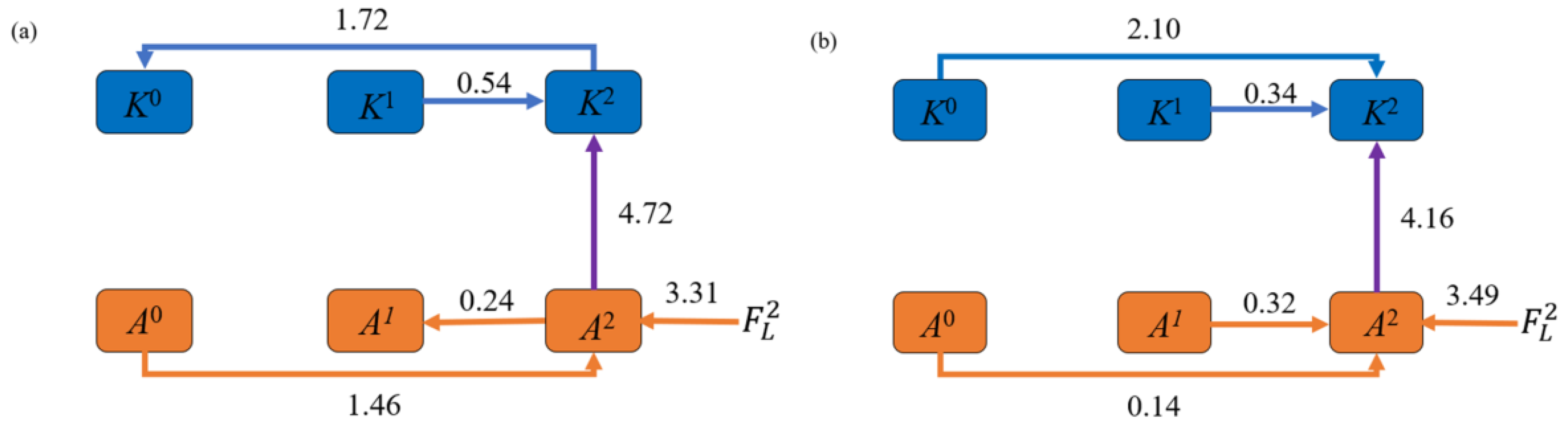
5.3. Energy Pathway
5.4. Comparison between Stage I and Stage II
6. Conclusions
Author Contributions
Funding
Institutional Review Board Statement
Informed Consent Statement
Data Availability Statement
Acknowledgments
Conflicts of Interest
References
- Zhu, Y.; Newell, R.E. A Proposed Algorithm for Moisture Fluxes from Atmospheric Rivers. Mon. Weather Rev. 1998, 126, 725–735. [Google Scholar] [CrossRef]
- Guan, B.; Waliser, D.E. Detection of Atmospheric Rivers: Evaluation and Application of an Algorithm for Global Studies. J. Geophys. Res. Atmos. 2015, 120, 12514–12535. [Google Scholar] [CrossRef]
- Dettinger, M.D.; Ralph, F.M.; Das, T.; Neiman, P.J.; Cayan, D.R. Atmospheric Rivers, Floods and the Water Resources of California. Water 2011, 3, 445–478. [Google Scholar] [CrossRef]
- Paltan, H.; Waliser, D.; Lim, W.H.; Guan, B.; Yamazaki, D.; Pant, R.; Dadson, S. Global Floods and Water Availability Driven by Atmospheric Rivers. Geophys. Res. Lett. 2017, 44, 10387–10395. [Google Scholar] [CrossRef]
- Xiong, Y.; Ren, X. Influences of Atmospheric Rivers on North Pacific Winter Precipitation: Climatology and Dependence on ENSO Condition. J. Clim. 2021, 34, 277–292. [Google Scholar] [CrossRef]
- Ralph, F.M.; Neiman, P.J.; Wick, G.A.; Gutman, S.I.; Dettinger, M.D.; Cayan, D.R.; White, A.B. Flooding on California’s Russian River: Role of Atmospheric Rivers. Geophys. Res. Lett. 2006, 33, L13801. [Google Scholar] [CrossRef] [Green Version]
- Neiman, P.J.; Ralph, F.M.; Wick, G.A.; Lundquist, J.D.; Dettinger, M.D. Meteorological Characteristics and Overland Precipitation Impacts of Atmospheric Rivers Affecting the West Coast of North America Based on Eight Years of SSM/I Satellite Observations. J. Hydrometeorol. 2008, 9, 22–47. [Google Scholar] [CrossRef]
- Ralph, F.M.; Dettinger, M.D. Historical and National Perspectives on Extreme West Coast Precipitation Associated with Atmospheric Rivers during December 2010. Bull. Am. Meteorol. Soc. 2012, 93, 783–790. [Google Scholar] [CrossRef]
- Guan, B.; Molotch, N.P.; Waliser, D.E.; Fetzer, E.J.; Neiman, P.J. The 2010/2011 Snow Season in California’s Sierra Nevada: Role of Atmospheric Rivers and Modes of Large-scale Variability. Water Resour. Res. 2013, 49, 6731–6743. [Google Scholar] [CrossRef]
- Lavers, D.A.; Villarini, G. The Nexus between Atmospheric Rivers and Extreme Precipitation across Europe. Geophys. Res. Lett. 2013, 40, 3259–3264. [Google Scholar] [CrossRef]
- Kim, J.; Moon, H.; Guan, B.; Waliser, D.E.; Choi, J.; Gu, T.; Byun, Y. Precipitation Characteristics Related to Atmospheric Rivers in East Asia. Int. J. Climatol. 2021, 41, E2244–E2257. [Google Scholar] [CrossRef]
- White, A.B.; Neiman, P.J.; Creamean, J.M.; Coleman, T.; Ralph, F.M.; Prather, K.A. The Impacts of California’s San Francisco Bay Area Gap on Precipitation Observed in the Sierra Nevada during HMT and CalWater. J. Hydrometeorol. 2015, 16, 1048–1069. [Google Scholar] [CrossRef] [Green Version]
- DeFlorio, M.J.; Waliser, D.E.; Guan, B.; Ralph, F.M.; Vitart, F. Global Evaluation of Atmospheric River Subseasonal Prediction Skill. Clim. Dyn. 2019, 52, 3039–3060. [Google Scholar] [CrossRef]
- Pan, M.; Lu, M. A Novel Atmospheric River Identification Algorithm. Water Resour. Res. 2019, 55, 6069–6087. [Google Scholar] [CrossRef]
- Pan, M.; Lu, M. East Asia Atmospheric River Catalog: Annual Cycle, Transition Mechanism and Precipitation. Geophys. Res. Lett. 2020, 47, e2020GL089477. [Google Scholar] [CrossRef]
- Fu, G.; Liu, S.; Li, X.; Li, P.; Chen, L. Characteristics of Atmospheric Rivers over the East Asia in Middle Summers from 2001 to 2016. J. Ocean Univ. China 2021, 20, 235–243. [Google Scholar] [CrossRef]
- Fu, G.; Liu, S.; Li, X.; Chen, L. Review on Atmospheric River Research. Period. Ocean Univ. China 2019, 49, 10–17. (In Chinese) [Google Scholar] [CrossRef]
- Kim, J. Precipitation and Snow Budget Over the Southwestern United States During the 1994–1995 Winter Season in a Mesoscale Model Simulation. Water Resour. Res. 1997, 33, 2831–2839. [Google Scholar] [CrossRef]
- Kamae, Y.; Mei, W.; Xie, S.-P. Climatological Relationship between Warm Season Atmospheric Rivers and Heavy Rainfall over East Asia. J. Meteorol. Soc. Jpn. 2017, 95, 411–431. [Google Scholar] [CrossRef] [Green Version]
- Konrad, C.P.; Dettinger, M.D. Flood Runoff in Relation to Water Vapor Transport by Atmospheric Rivers Over the Western United States, 1949–2015. Geophys. Res. Lett. 2017, 44, 11456–11462. [Google Scholar] [CrossRef] [Green Version]
- Trenberth, K. Atmospheric Moisture Recycling: Role of Advection and Local Evaporation. J. Clim. 1999, 12, 1368–1381. [Google Scholar] [CrossRef]
- Trenberth, K.; Smith, L.; Qian, T.; Dai, A.; Fasullo, J. Estimates of the Global Water Budget and Its Annual Cycle Using Observational and Model Data. J. Hydrometeorol. 2007, 8, 758–769. [Google Scholar] [CrossRef]
- Ralph, F.M.; Neiman, P.J.; Kiladis, G.N.; Weickmann, K.; Reynolds, D.W. A Multiscale Observational Case Study of a Pacific Atmospheric River Exhibiting Tropical–Extratropical Connections and a Mesoscale Frontal Wave. Mon. Weather Rev. 2011, 139, 1169–1189. [Google Scholar] [CrossRef]
- Liang, X.S. Canonical Transfer and Multiscale Energetics for Primitive and Quasigeostrophic Atmospheres. J. Atmos. Sci. 2016, 73, 4439–4468. [Google Scholar] [CrossRef] [Green Version]
- Liang, X.S.; Anderson, D.G.M. Multiscale Window Transform. Multiscale Model. Simul. 2007, 6, 437–467. [Google Scholar] [CrossRef]
- Hersbach, H.; Bell, B.; Berrisford, P.; Hirahara, S.; Horányi, A.; Muñoz-Sabater, J.; Nicolas, J.; Peubey, C.; Radu, R.; Schepers, D.; et al. The ERA5 Global Reanalysis. Q. J. R. Meteorol. Soc. 2020, 146, 1999–2049. [Google Scholar] [CrossRef]
- Lorenz, E.N. Available Potential Energy and the Maintenance of the General Circulation. Tellus 1955, 7, 157–167. [Google Scholar] [CrossRef] [Green Version]
- Shen, Y.; Sun, Y.; Liu, D.Y. Effect of Condensation Latent Heat Release on the Relative Vorticity Tendency in Extratropical Cyclones: A Case Study. Atmos. Ocean. Sci. Lett. 2020, 13, 275–285. [Google Scholar] [CrossRef]
- Liang, X.S.; Robinson, A.R. Localized Multiscale Energy and Vorticity Analysis I. Fundamentals. Dyn. Atmos. Oceans 2005, 38, 195–230. [Google Scholar] [CrossRef]
- Liang, X.S.; Robinson, A.R. Localized Multi-Scale Energy and Vorticity Analysis II. Finite-Amplitude Instability Theory and Validation. Dyn. Atmos. Oceans 2007, 44, 51–76. [Google Scholar] [CrossRef]
- Xu, F.; Liang, X.S. The Synchronization between the Zonal Jet Stream and Temperature Anomalies Leads to an Extremely Freezing North America in January 2019. Geophys. Res. Lett. 2020, 47, e2020GL089689. [Google Scholar] [CrossRef]
- Zhao, Y.-B.; Liang, X.S. On the Inverse Relationship between the Boreal Wintertime Pacific Jet Strength and Storm-Track Intensity. J. Clim. 2018, 31, 9545–9564. [Google Scholar] [CrossRef]
- Ma, J.; Liang, X.S. Multiscale Dynamical Processes Underlying the Wintertime Atlantic Blockings. J. Atmos. Sci. 2017, 74, 3815–3831. [Google Scholar] [CrossRef]
- Xu, F.; Liang, X.S. Drastic Change in Dynamics as Typhoon Lekima Experiences an Eyewall Replacement Cycle. Front. Earth Sci. 2021, 1–11. [Google Scholar] [CrossRef]
- Rong, Y.-N.; Ma, J.; Li, Y.; Liang, X.S. On the Multiscale Dynamics of a Top-down Developing Vortex over Tibet Plateu. Adv. Meteorol. Sci. Technol. 2021, 11, 7–18. (In Chinese) [Google Scholar] [CrossRef]
- Yang, Y.; Liang, X.S. New Perspectives on the Generation and Maintenance of the Kuroshio Large Meander. J. Phys. Oceanogr. 2019, 49, 2095–2113. [Google Scholar] [CrossRef]
- Rutz, J.J.; Steenburgh, W.J.; Ralph, F.M. Climatological Characteristics of Atmospheric Rivers and Their Inland Penetration over the Western United States. Mon. Weather Rev. 2014, 142, 905–921. [Google Scholar] [CrossRef]
- Ralph, F.M.; Rutz, J.J.; Cordeira, J.M.; Dettinger, M.; Anderson, M.; Reynolds, D.; Schick, L.J.; Smallcomb, C. A Scale to Characterize the Strength and Impacts of Atmospheric Rivers. Bull. Am. Meteorol. Soc. 2019, 100, 269–289. [Google Scholar] [CrossRef]
- Newell, R.E.; Newell, N.E.; Zhu, Y.; Scott, C. Tropospheric Rivers?—A Pilot Study. Geophys. Res. Lett. 1992, 19, 2401–2404. [Google Scholar] [CrossRef] [Green Version]
- Ralph, F.M.; Neiman, P.J.; Wick, G.A. Satellite and CALJET Aircraft Observations of Atmospheric Rivers over the Eastern North Pacific Ocean during the Winter of 1997/98. Mon. Weather Rev. 2004, 132, 1721–1745. [Google Scholar] [CrossRef] [Green Version]
- Torrence, C.; Compo, G.P. A Practical Guide to Wavelet Analysis. Bull. Am. Meteorol. Soc. 1998, 79, 61–78. [Google Scholar] [CrossRef] [Green Version]
- Gimeno, L.; Nieto, R.; Vázquez, M.; Lavers, D.A. Atmospheric Rivers: A Mini-Review. Front. Earth Sci. 2014, 2, 1–6. [Google Scholar] [CrossRef]


Publisher’s Note: MDPI stays neutral with regard to jurisdictional claims in published maps and institutional affiliations. |
© 2021 by the authors. Licensee MDPI, Basel, Switzerland. This article is an open access article distributed under the terms and conditions of the Creative Commons Attribution (CC BY) license (https://creativecommons.org/licenses/by/4.0/).
Share and Cite
Zhang, Z.; Liang, X.S. Multiscale Interactive Processes Underlying the Heavy Rainstorm Associated with a Landfalling Atmospheric River. Atmosphere 2022, 13, 29. https://doi.org/10.3390/atmos13010029
Zhang Z, Liang XS. Multiscale Interactive Processes Underlying the Heavy Rainstorm Associated with a Landfalling Atmospheric River. Atmosphere. 2022; 13(1):29. https://doi.org/10.3390/atmos13010029
Chicago/Turabian StyleZhang, Zhuang, and X. San Liang. 2022. "Multiscale Interactive Processes Underlying the Heavy Rainstorm Associated with a Landfalling Atmospheric River" Atmosphere 13, no. 1: 29. https://doi.org/10.3390/atmos13010029