
Forecasting GNSS Zenith Troposphere Delay by Improving GPT3 Model with Machine Learning in Antarctica


Abstract
:1. Introduction
2. Data and Methodology
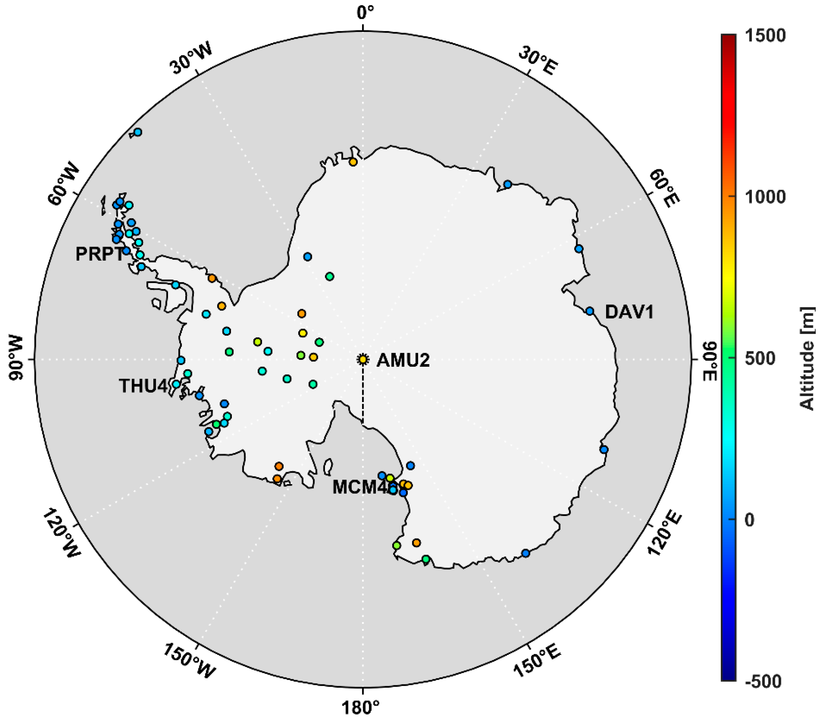
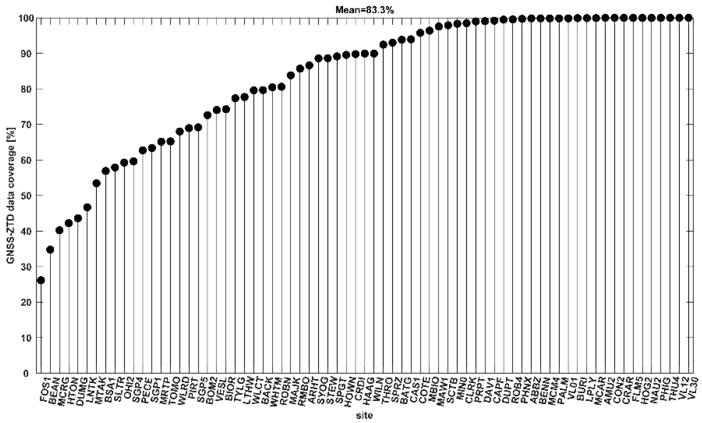
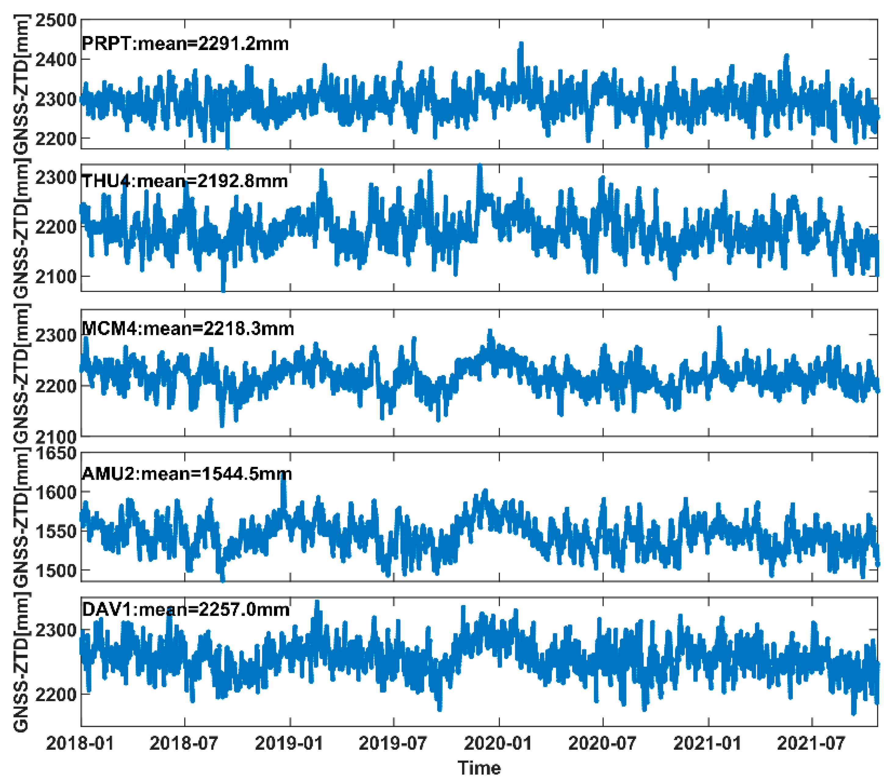
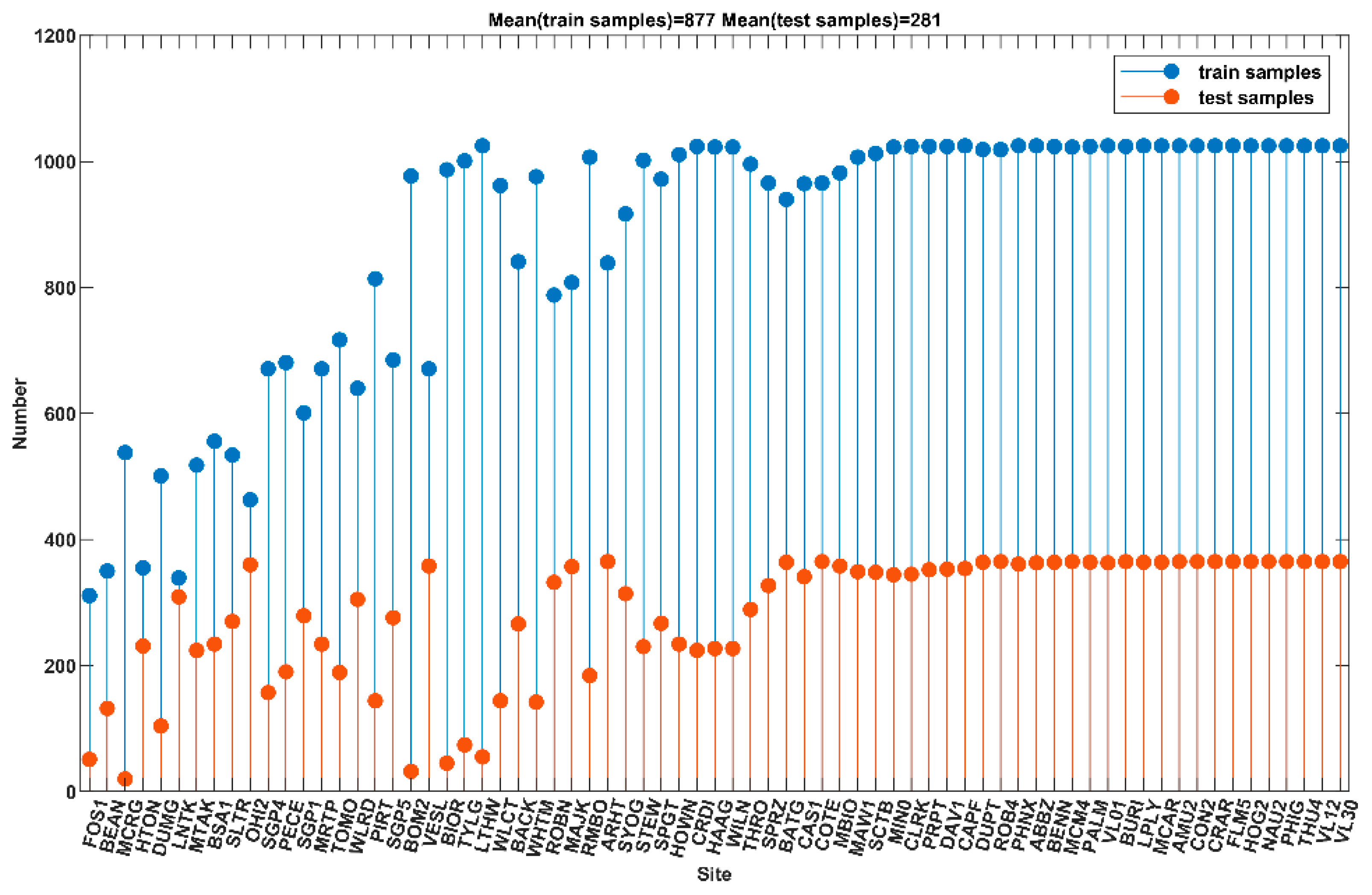
2.1. Data Source
2.2. Method for Determining ZTD
2.2.1. GPT3_ZTD
2.2.2. LSTM_ZTD
2.2.3. LSTM_RBF_ZTD
2.3. Verification
3. Results
3.1. Accuracy of the LSTM_ZTD
3.2. Comparisons between the LSTM_RBF_ZTD and the GPT3_ZTD
4. Discussion
5. Conclusions
Author Contributions
Funding
Institutional Review Board Statement
Informed Consent Statement
Data Availability Statement
Acknowledgments
Conflicts of Interest
References
- Suparta, W.; Abdul Rashid, Z.A.; Mohd Ali, M.A.; Yatim, B.; Fraser, G.J. Observations of Antarctic precipitable water vapor and its response to the solar activity based on GPS sensing. J. Atmos. Sol. Terr. Phys. 2008, 70, 1419–1447. [Google Scholar] [CrossRef]
- Vázquez, B.G.E.; Grejner-Brzezinska, D.A. GPS-PWV estimation and validation with radiosonde data and numerical weather prediction model in Antarctica. GPS Solut. 2012, 17, 29–39. [Google Scholar] [CrossRef]
- Li, W.; Yuan, Y.; Ou, J.; Li, H.; Li, Z. A new global zenith tropospheric delay model IGGtrop for GNSS applications. Chin. Sci. Bull. 2012, 57, 2132–2139. [Google Scholar] [CrossRef] [Green Version]
- Li, W.; Yuan, Y.; Ou, J.; He, Y. IGGtrop_SH and IGGtrop_rH: Two Improved Empirical Tropospheric Delay Models Based on Vertical Reduction Functions. IEEE Trans. Geosci. Remote Sens. 2018, 56, 5276–5288. [Google Scholar] [CrossRef]
- Li, W.; Yuan, Y.; Ou, J.; Chai, Y.; Li, Z.; Liou, Y.-A.; Wang, N. New versions of the BDS/GNSS zenith tropospheric delay model IGGtrop. J. Geod. 2014, 89, 73–80. [Google Scholar] [CrossRef]
- Yao, Y.; Xu, C.; Zhang, B.; Cao, N. A global empirical model for mapping zenith wet delays onto precipitable water vapor using GGOS Atmosphere data. Sci. China Earth Sci. 2015, 58, 1361–1369. [Google Scholar] [CrossRef]
- Yao, Y.; Hu, Y.; Yu, C.; Zhang, B.; Guo, J. An improved global zenith tropospheric delay model GZTD2 considering diurnal variations. Nonlinear Processes Geophys. 2016, 23, 127–136. [Google Scholar] [CrossRef] [Green Version]
- Sun, L.; Chen, P.; Wei, E.; Li, Q. Global model of zenith tropospheric delay proposed based on EOF analysis. Adv. Space Res. 2017, 60, 187–198. [Google Scholar] [CrossRef]
- Wang, S.; Xu, T.; Nie, W.; Jiang, C.; Yang, Y.; Fang, Z.; Li, M.; Zhang, Z. Evaluation of Precipitable Water Vapor from Five Reanalysis Products with Ground-Based GNSS Observations. Remote Sens. 2020, 12, 1817. [Google Scholar] [CrossRef]
- Li, S.; Xu, T.; Jiang, N.; Yang, H.; Wang, S.; Zhang, Z. Regional Zenith Tropospheric Delay Modeling Based on Least Squares Support Vector Machine Using GNSS and ERA5 Data. Remote Sens. 2021, 13, 1004. [Google Scholar] [CrossRef]
- Huang, L.; Mo, Z.; Liu, L.; Zeng, Z.; Chen, J.; Xiong, S.; He, H. Evaluation of Hourly PWV Products Derived From ERA5 and MERRA-2 Over the Tibetan Plateau Using Ground-Based GNSS Observations by Two Enhanced Models. Earth Space Sci. 2021, 8, e2020EA001516. [Google Scholar] [CrossRef]
- Jiang, C.; Xu, T.; Wang, S.; Nie, W.; Sun, Z. Evaluation of Zenith Tropospheric Delay Derived from ERA5 Data over China Using GNSS Observations. Remote Sens. 2020, 12, 663. [Google Scholar] [CrossRef] [Green Version]
- Huang, L.; Guo, L.; Liu, L.; Chen, H.; Chen, J.; Xie, S. Evaluation of the ZWD/ZTD Values Derived from MERRA-2 Global Reanalysis Products Using GNSS Observations and Radiosonde Data. Sensors 2020, 20, 6440. [Google Scholar] [CrossRef] [PubMed]
- Huang, L.; Zhu, G.; Liu, L.; Chen, H.; Jiang, W. A global grid model for the correction of the vertical zenith total delay based on a sliding window algorithm. GPS Solut. 2021, 25, 98. [Google Scholar] [CrossRef]
- Leandro, R.F.; Langley, R.B.; Santos, M.C. UNB3m_pack: A neutral atmosphere delay package for radiometric space techniques. GPS Solut. 2007, 12, 65–70. [Google Scholar] [CrossRef]
- Penna, N.; Dodson, A.; Chen, W. Assessment of EGNOS Tropospheric Correction Model. J. Navig. 2001, 54, 37–55. [Google Scholar] [CrossRef] [Green Version]
- Schuh, J.B.R.H.H. Short Note: A global model of pressure and temperature for geodetic applications. J. Geod. 2007, 81, 679–683. [Google Scholar] [CrossRef]
- Böhm, J.; Möller, G.; Schindelegger, M.; Pain, G.; Weber, R. Development of an improved empirical model for slant delays in the troposphere (GPT2w). GPS Solut. 2014, 19, 433–441. [Google Scholar] [CrossRef] [Green Version]
- Lagler, K.; Schindelegger, M.; Bohm, J.; Krasna, H.; Nilsson, T. GPT2: Empirical slant delay model for radio space geodetic techniques. Geophys. Res. Lett. 2013, 40, 1069–1073. [Google Scholar] [CrossRef] [Green Version]
- Landskron, D.; Bohm, J. VMF3/GPT3: Refined discrete and empirical troposphere mapping functions. J. Geod. 2018, 92, 349–360. [Google Scholar] [CrossRef] [PubMed]
- Yibin, Y.; Na, C.; Chaoqian, X.; Junjian, Y. Accuracy Assessment and Analysis for GPT2. Acta Geod. Cartogr. Sin. 2015, 44, 726–733. [Google Scholar] [CrossRef]
- Jian, K.; Yibin, Y.; Lulu, S.; Zemin, W. The Accuracy Analysis of GPT2w at the Antarctic Area. Acta Geod. Cartogr. Sin. 2018, 47, 1316–1325. [Google Scholar] [CrossRef]
- Yang, F.; Guo, J.; Meng, X.; Li, J.; Zou, J.; Xu, Y. Establishment and assessment of a zenith wet delay (ZWD) augmentation model. GPS Solut. 2021, 25, 148. [Google Scholar] [CrossRef]
- Zhang, Q.; Li, F.; Zhang, S.; Li, W. Modeling and Forecasting the GPS Zenith Troposphere Delay in West Antarctica Based on Different Blind Source Separation Methods and Deep Learning. Sensors 2020, 20, 2343. [Google Scholar] [CrossRef] [Green Version]
- Du, Z.; Zhao, Q.; Yao, W.; Yao, Y. Improved GPT2w (IGPT2w) model for site specific zenith tropospheric delay estimation in China. J. Atmos. Sol.-Terr. Phys. 2020, 198, 105202. [Google Scholar] [CrossRef]
- Blewitt, G.; Hammond, W.C.; Kreemer, C. Harnessing the GPS data explosion for interdisciplinary science. Eos 2018, 99, 485. [Google Scholar] [CrossRef]
- Ding, J.; Chen, J. Assessment of Empirical Troposphere Model GPT3 Based on NGL’s Global Troposphere Products. Sensors 2020, 20, 3631. [Google Scholar] [CrossRef]
- Saastamoinen, J. Atmospheric Correction for the Troposphere and Stratosphere in Radio Ranging Satellites. In Use of Aritificial Satellites for Geodesy; Wiley: Hoboken, NJ, USA, 1972; Volume 15. [Google Scholar]
- Askne, J.; Nordius, H. Estimation of tropospheric delay for microwaves from surface weather data. Radio Sci. 1987, 22, 379–386. [Google Scholar] [CrossRef]
- Hochreiter, S.; Schmidhuber, J. Long short-term memory. Neural. Comput. 1997, 9, 1735–1780. [Google Scholar] [CrossRef]
- Broomhead, D.S. Multivar iable Functional Interpolation and Adaptive Networks. Complex Syst. 1988, 2, 321–355. [Google Scholar]


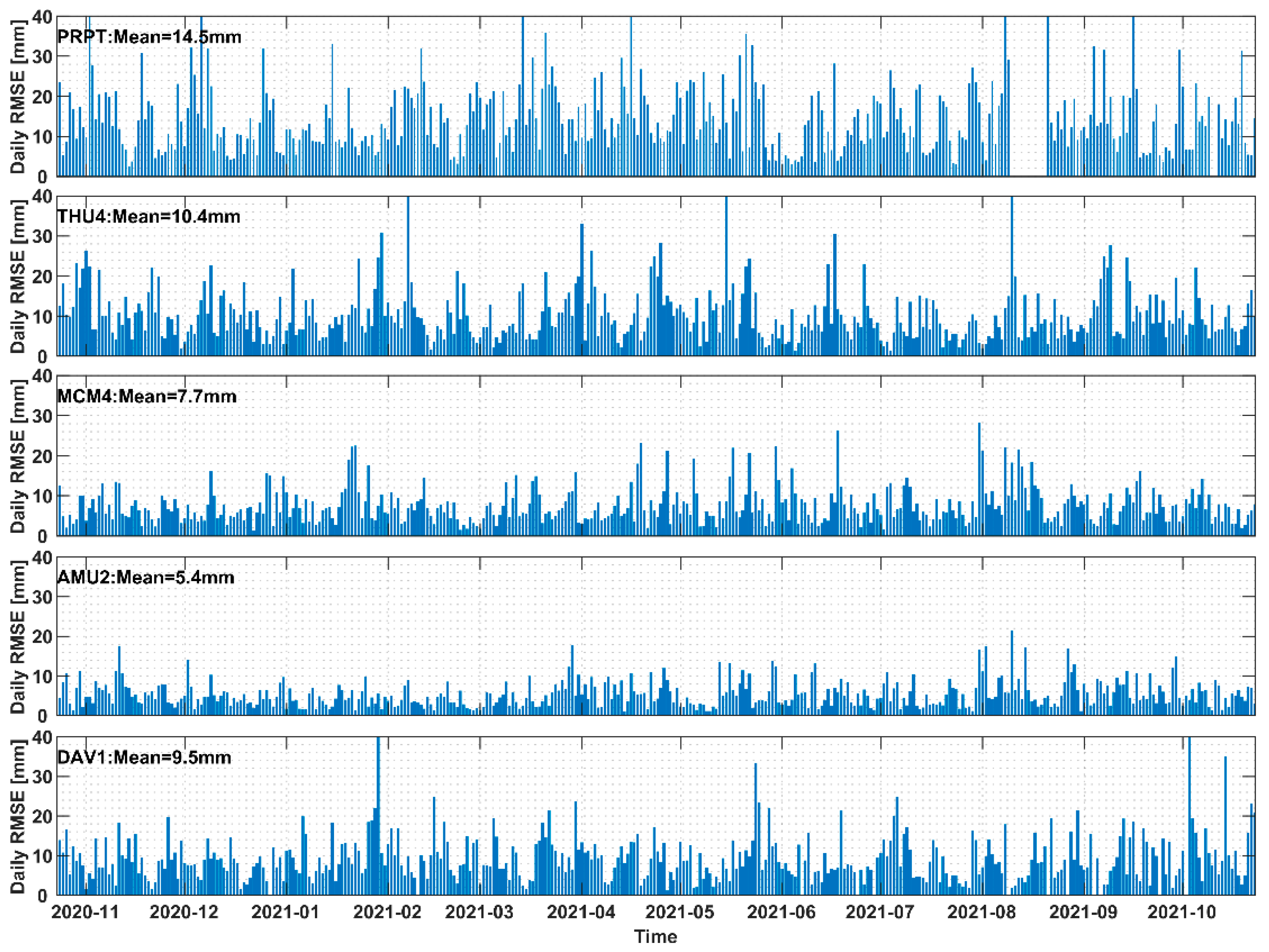
| Daily RMSE | 0–5 mm | 5–10 mm | >10 mm |
|---|---|---|---|
| PRPT | 26 | 104 | 222 |
| THU4 | 70 | 143 | 152 |
| MCM4 | 115 | 166 | 84 |
| AMU2 | 193 | 133 | 39 |
| DAV1 | 73 | 150 | 130 |
| mean | 95.4 | 139.2 | 125.4 |
| RMSE | Number of sites | |
|---|---|---|
| Yearly RMSE | 5–10 mm | 40 |
| 10–15 mm | 14 | |
| 15–20 mm | 9 | |
| >20 mm | 2 | |
| Daily RMSE | 50% < 10 mm | 50 |
| 75% < 10 mm | 35 | |
| 50% < 20 mm | 63 | |
| 75% < 20 mm | 63 |
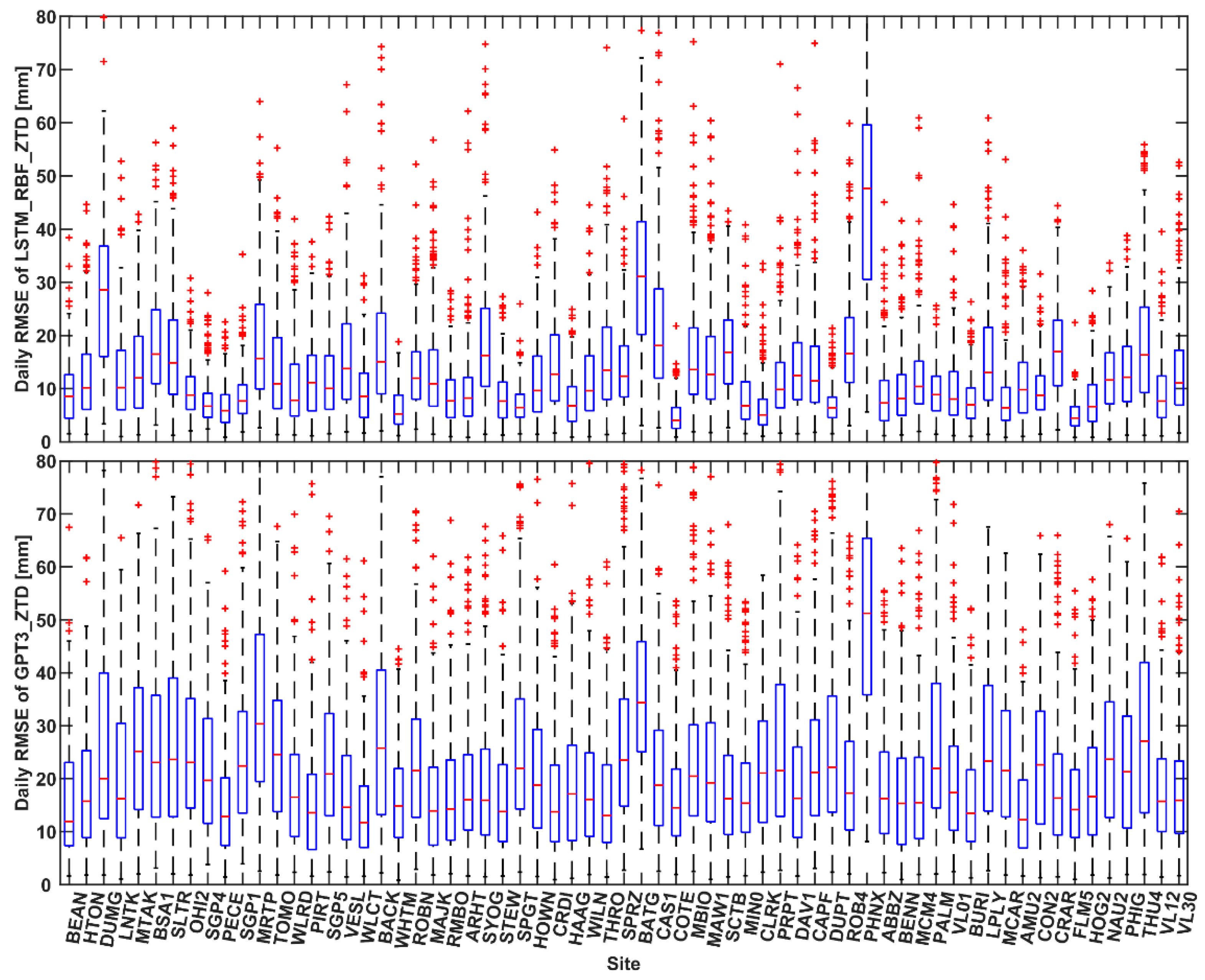
| Daily RMSE | LSTM_RBF_ZTD | GPT3_ZTD |
|---|---|---|
| 50% < 10 mm | 31 | 0 |
| 75% < 10 mm | 8 | 0 |
| 50% < 20 mm | 62 | 39 |
| 75% < 20 mm | 47 | 2 |
| Yearly RMSE | LSTM_RBF_ZTD | GPT3_ZTD |
|---|---|---|
| 0–10 mm | 12 | 0 |
| 10–20 mm | 40 | 8 |
| 20–30 mm | 10 | 41 |
| >30 mm | 3 | 16 |
Publisher’s Note: MDPI stays neutral with regard to jurisdictional claims in published maps and institutional affiliations. |
© 2022 by the authors. Licensee MDPI, Basel, Switzerland. This article is an open access article distributed under the terms and conditions of the Creative Commons Attribution (CC BY) license (https://creativecommons.org/licenses/by/4.0/).
Share and Cite
Li, S.; Xu, T.; Xu, Y.; Jiang, N.; Bastos, L. Forecasting GNSS Zenith Troposphere Delay by Improving GPT3 Model with Machine Learning in Antarctica. Atmosphere 2022, 13, 78. https://doi.org/10.3390/atmos13010078
Li S, Xu T, Xu Y, Jiang N, Bastos L. Forecasting GNSS Zenith Troposphere Delay by Improving GPT3 Model with Machine Learning in Antarctica. Atmosphere. 2022; 13(1):78. https://doi.org/10.3390/atmos13010078
Chicago/Turabian StyleLi, Song, Tianhe Xu, Yan Xu, Nan Jiang, and Luísa Bastos. 2022. "Forecasting GNSS Zenith Troposphere Delay by Improving GPT3 Model with Machine Learning in Antarctica" Atmosphere 13, no. 1: 78. https://doi.org/10.3390/atmos13010078