Abstract
In this study, five simulations were conducted using the weather research and forecasting (WRF) model with different cumulus parameterizations schemes (CPSs) for the period from 2013 until 2018. A one-year simulation of 2013 with three different horizontal resolutions of 25, 5, and 1.6 km was also performed. The CPSs used were Kain–Fritsch (KF), Grell–Devenyi (GR), Betts–Miller–Janjic (BM), and a non-parameterized scheme (NC). In assessments of model resolutions, both the 25 and 5 km resolutions depicted a strong negative bias in the northeastern part of Peninsular Malaysia during December–January–February (DJF), with marginal differences between the two simulations. Among all 5 km experiments, the best performing scheme was the BM scheme for almost all seasons. Furthermore, the 5 km simulation did not exhibit significant differences relative to the 25 km of the diurnal cycle. The 1.6 km simulation showed significant added value as it was the only simulation that was able to simulate the high precipitation intensity in the morning and a precipitation peak during the evening. The 1.6 km resolution was also the only resolution capable of picking up the precipitation signals in the R4 region (South Peninsular Malaysia) compared to the other two resolutions. While both CPSs and resolutions are important for accurate predictions, the role of CPSs became less significant in a higher resolution simulation.
1. Introduction
Climate models are an essential tool for the study of climate change. It can be described as a numerical equation that represents the interaction between the atmosphere, the land, and the ocean with the first ever successful climate model being constructed in 1956 [1]. With the advancement of technology and cooperation between scientists having become the norm, climate models have become a reliable tool for climate scientists following the creation of the first regional climate model (RCM) in 1989 using a nested downscaling method [2,3]. Today, high-resolution climate models reaching a 1 km resolution can be produced. As such, this work discusses the capability and performance of the weather research and forecasting model (WRF), which is one of the most widely used RCMs in climate modeling. Despite that, the model alone is not enough to simulate the climate perfectly as some climate events are too small for the model to capture. It depends on the resolution of the model itself. Hence, physical parameterizations are needed to circumvent this weakness. Physical parameterization functions by replacing the physical processes that are too small for the model to capture and simulate. One of the most important physical parameterizations in simulating precipitation are clouds. Most clouds have an area of less than 1 km and simulating climate at a high resolution is computationally consuming. Hence, these clouds are parameterized into the model with varying configurations and equations known as cumulus parameterization schemes (CPSs).
CPSs provide a representation of shallow and deep cumulus clouds and are an integral component in simulating precipitation. The CPSs are represented by simulating deep and shallow convection, and each CPS has different trigger functions such as focusing on shallow schemes while ignoring deep cumulus clouds or vice versa [4]. Many CPSs are available, and each differs from one model to another as they are constructed according to what the developers think is the most important. As a rule of thumb, the settings of CPSs must be able to determine three important criteria, namely, the intensity, presence, and impact of cumulus clouds. Determining which parameterization suits which region is a daunting task as it changes as the resolution increases [5]. Despite the difficulty of using high-resolution simulations, multiple evaluations in the tropical region of Southeast Asia using different models and CPSs have shown that simulation resolutions of 25 km and lower are not enough to fully simulate the climatology of Southeast Asia. Ratna et al. [6] used a 27 km resolution WRF and showed that Malaysia had a significant negative precipitation bias over Peninsular Malaysia during December–January–February (DJF). The eastern part of Peninsular Malaysia was supposed to experience a significant amount of rainfall during the DJF season because of the northeast monsoon, but the WRF model was unable to replicate the full effect of the monsoon. This problem is not limited to the WRF; it is also prevalent in other climate models such as the regional climate model system (RegCM4) and the fifth-generation Penn State/NCAR mesoscale model (MM5) by Juneng et al. [7] and Salimun et al. [8], respectively. The resolution and CPS are possible issues that hinder the performances of these climate models because the rainfall mechanisms in Peninsular Malaysia are affected by multiple large-scale events such as the Madden–Julian Oscillation (MJO), the El Niño–Southern Oscillation (ENSO), and the Indonesian Throughflow (ITF) [9].
Hence, analyzing the performances of the WRF models at a high resolution could prove useful in simulating precipitation events in Peninsular Malaysia. Resolutions reaching 10 km and below are known as gray zones. Originally, the term was known as ‘Terra Incognita’, which describes a state where atmospheric motions can be resolved fully or partially using a model grid. The 1–10 km range is important in climate studies due to the difficulty of resolving convection and boundary-layer turbulence with a coarse resolution. Turbulence has features ranging from 1 km to 100 m, while moist convection occurs over scales of around 1–10 km [10]. By the year 2007, this range was widely known as the gray zone, illustrating our limited understanding of the inner workings of the high-resolution phenomenon [11]. One such example is the convoluted boundary layer in the gray zone being heavily impacted by the changes in potential temperature perturbations [12]. Working out a model simulation in the gray zone has additional problems relating to computational power and the usage of cumulus parameterizations at this resolution. Scientists must decide if an increase in resolution is worth the computational stress. Through experiments, Schwartz et al. [13] and Kain et al. [14] concluded that an increase in resolution is not worth increasing computational costs as the results do not produce enough benefits to counteract the amount of time and space required to run the model. Hence, scientists must find a valid reason to run a high-resolution and demanding simulation. The inclusion of cumulus parameterizations in the gray zone is also a highly debated subject. In fact, a study by Field et al. [15] concluded that atmospheric instability was being removed too easily by the conventional convection parameterization, which prevents the models from resolving the vertical composition of the atmosphere at a high resolution. However, there is some benefit to the use of high-resolution simulations, as shown by Petch et al. [16] and Bryan et al. [17] who suggested that resolutions smaller than 1 km were needed to predict convective systems. Furthermore, a study by Holloway et al. [18] over land and the tropical Pacific Ocean revealed that a higher resolution provided a better representation of precipitation and clouds.
Cumulus parameterization schemes (CPS) provide a representation of shallow and deep cumulus clouds and are an integral component in simulating precipitation. This method functions by simulating deep and shallow convection, and each CPS has different trigger functions such as focusing on shallow schemes while ignoring deep cumulus clouds or vice versa [13]. Additionally, convection or deep cumulus clouds usually have a horizontal scale of 10 km, and a 5 km horizontal grid spacing can thus hypothetically resolve convection. However, shallow convection has a horizontal scale of 1 km or less which makes its parameterization difficult [19]. Another problem to consider is that the usage of CPSs in high-resolution simulations violates the underlying assumptions and hypotheses made by Arakawa and Chen [20] and Hammarstrand [21]. This was because most of the CPSs were designed with the assumption that the horizontal grid interval of the model is higher than the spatial scale of the convective updraft. Nevertheless, scientists have tested the function of CPSs in the gray area. For example, Deng and Stuffer [22] showed that using CPS greatly decreased the problem of grid-point storms at a 4 km resolution. Similarly, a 2 km thunderstorm simulation by Kotroni and Lagouvardos [23] also supported the use of CPSs in gray areas. Despite the difficulty of using high-resolution simulations, multiple evaluations in the tropical region of Southeast Asia using different models have shown that simulation resolutions of 25 km and lower are not enough to fully simulate the climatology of Southeast Asia. The resolution and CPS are possible issues that hinder the performances of these climate models because the rainfall mechanisms in Peninsular Malaysia are affected by multiple mesoscale events such as the Madden–Julian Oscillation (MJO), the El Niño–Southern Oscillation (ENSO), and the Indonesian Throughflow (ITF) [22]. Hence, this study aimed to further test the capability of the CPS of the WRF model in simulating rainfall in a tropical climate at a high resolution, in order to provide additional results and come closer to solving the mystery of the gray zone. Considering the drawbacks of high-resolution studies, we compromised with the computational restrictions at hand and tried to identify the best CPSs to simulate high-resolution models. In addition, we further investigated the capabilities of these different horizontal resolutions for the capture of local features such as diurnal phenomena.
2. Materials and Methods
2.1. Experimental Design
The WRF model was used in this experiment, which was designed by the National Centre of Atmospheric Research (NCAR) with the capability of simulating both idealized and real data applications [24]. This model can implement a variety of physical options that cater to both long and short simulations. This experiment had three domains with horizontal resolutions of 25 (Domain 1), 5, (Domain 2), and 1.6 km (Domain 3). The simulation was run over 5 years from 2013 to 2018 with a spin-up time of one year, while the 1.6 km simulation only covered a one-year simulation of 2013 with a spin-up time of two months. The simulations were set up to run in a non-hydrostatic mode with initial and boundary conditions provided by the European Center for Medium-Range Weather Forecasting (ECMWF) reanalysis (ERA-Interim). ECMWF reanalysis was used because it is one of the best performed reanalysis models in the Southeast Asia (SEA) domain [5]. Domain 1 covered the whole of Southeast Asia following the spatial design by CORDEX Southeast Asia, while Domain 2 covered Peninsular Malaysia; Domain 3 was a little bit smaller than the second to provide breathing room for the leaking of boundary conditions (Figure 1).
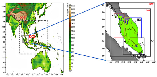
Figure 1.
Experimental domain configurations. D01, D02, and D03 have resolutions of 25, 5, and 1.6 km, respectively.
Borneo Island was not included in this experiment purely due to the computational costs of running a high-resolution study. An initial test was conducted to determine computational costs and the results showed that a one-year simulation cost almost one terabyte of storage. Hence, only the area of Peninsular Malaysia was considered in this study. There were three stages in conducting this experiment. First, the CPSs in the 5 km resolution simulation were compared to find the best performing CPS. Next, we compared the 5 and 25 km resolutions with every setting kept the same so that the only variable to compare was the difference in the resolution. Finally, the 25, 5, and 1.6 km resolutions were compared to investigate if there was any added value in using a finer resolution for diurnal analyses.
The physics configuration used in this experiment follows the same settings as the WRF model validation experiment conducted by Ratna et al. [6] in Southeast Asia except for the selections of CPSs (Table 1). Default WRF land surface model (LSM) 21-MODIS IGBP 21-category data were used in this experiment. The CPSs used in this study included the Kain–Fritsch (KF), Betts–Miller–Janjic (BM), Grell–Devenyi (GR), and Non-cumulus (NC) CPSs. The KF scheme is a deep and shallow sub-grid scheme using a mass flux approach [25]; the BM scheme is an adjustment scheme for deep and shallow convection where the thermodynamic considerations determine the temperature and humidity profile [26]; the GR ensemble scheme is a 144 sub-grid ensemble method that is both multi-closure and multi-parameter [27]; and the NC run is a simulation which does not use a cumulus parameterization scheme. NC runs were included because the behavior of CPSs change as the resolution increases; as shown in a study conducted by Jeworrek et al. [28], some CPSs were inactive when they reached a high-resolution simulation and produced the same result as an NC run. Due to the computational restriction, in this study, we separated the effect of resolutions and CPSs to achieve a better understanding of CPSs in a high-resolution simulation. However, additional research on the combined impact of CPSs and resolution is required in future studies.

Table 1.
Physics Configuration of WRF Model as compared to Ratna et al. [6].
2.2. Model Validation Method
The evaluation of the WRF model performances was based on a comparison of the model results and two observational data records. The data obtained from daily gridded precipitation records from the Climate Hazards Group InfraRed Precipitation with Station data (CHIRPS), the Tropical Rainfall Measuring Mission (TRMM), and 16 rain gauges located in Peninsular Malaysia are shown in Figure 1. The performances were evaluated by annual average and seasonal performances. The spatial evaluation was based on the bias comparison between the models and observational data with a 95% significance test. Taylor diagrams were included to check the performances of all simulations based on their root mean square error (RMSE), standard deviation (STD), and correlation (COR). The seasons were divided into four standard seasons, namely DJF (December, January, February), JJA (Jun, July, August), MAM (March, April, May), JJA (Jun, July, August), and SON (September, October, November). Additional significance tests were conducted at a 95% confidence in the bias of each season. Indeed, precipitation in Malaysia is strongly affected by two monsoon seasons: the northeast monsoon that occurs from October to March and the southwest monsoon, which begins around May and ends in September. The effects of these monsoons differ from region to region due to the position of the Titiwangsa Range in the center of Peninsular Malaysia. Hence, the area was divided into four distinct regions, as shown in Figure 1. Additionally, it is common to focus only on annual and seasonal analyses in evaluation studies of long-term simulations due to limited data sampling rates and sparse observational networks. However, diurnal precipitation is crucial for the proper evaluation of clouds and precipitation in tropical countries such as Malaysia since daily precipitation in Peninsular Malaysia is heavily affected by large-scale events such as the El Niño Southern Oscillation (ENSO), which is due to the temperature gradient differences in the Pacific Ocean. The ENSO evolves northeastward through the Pacific Ocean starting from JJA season. During DJF season, the ENSO would suppress the precipitation around Peninsular Malaysia [29]. Indian Ocean Dipole (IOD), on the other hand, is the Indian Ocean counterpart that could positively and negatively influence the precipitation intensity of Peninsular Malaysia as it converges with the ENSO event [30]. Precipitation in Peninsular Malaysia is also heavily affected by intraseasonal events such as the Madden-Julian Oscillation (MJO). The MJO has 8 phases that can be separated into dry and wet phases. The wet phase occurs around phase 1–3 and the dry phase occurs in phase 4–8 in Peninsular Malaysia [31]. In addition, Peninsular Malaysia has well-documented rain gauges spread throughout the country that have been operating for more than 50 years. As a result, diurnal analyses with 95% confidence intervals (shaded error plot) were conducted based on station data provided by the Malaysian Meteorological Department (MMD).
3. Results & Discussion
3.1. Cumulus Evaluation
For the first experiment, we focused on the 5 km resolution to determine whether the changes in CPSs would have a significant impact on the results. Figure 2 shows the means and biases of the spatial patterns of seasonal precipitation for all CPS experiments (BM, KF, GR, and NC) using the CHIRPS observational data. In Figure 2, the DJF season is shown on the first row, which consists of the results for CHIRPS: (a), BM (e), KF (i), GR (m), NC (q), BM-Bias (u), KF-Bias (y), GR-Bias (cc), and NC-bias (gg). During the DJF season, all CPS experiments were unable to capture the amount of heavy precipitation during the northeast monsoon with a high significance along the northeast of Peninsular Malaysia. From Figure 3 and Figure 4, both TRMM and CHIRPS were able to closely simulate the pattern of precipitation annually and seasonally throughout the region with a slight overestimation of rainfall intensity. Observational data also show the same underestimation of precipitation in the R3 Region during November and December. This correlates with a study done by [32], where both CHIRPS and TRMM have a tendency to overestimate monthly precipitation but underestimate the amount of precipitation during an extremely heavy rainfall event when compared with station data. The CPSs used were unable to produce the correct amounts of precipitation along the east coast and southern part of Peninsular Malaysia. The BM scheme was the second best at simulating high rainfall distributions in the eastern part of Peninsular Malaysia while the GR and NC runs tended to produce lower rainfall distributions. Both in Figure 2 and Figure 3, GR and NC revealed almost identical precipitation distribution results. The GR scheme produced a higher rainfall distribution than NC but at a very small rate and this could only be seen on the spatial scale and in the results of the root mean square error (RMSE), standard deviation (STD), and correlation (COR), as shown in Figure 4. The Taylor diagram showed that there is little difference between the GR and NC runs. There are a few reasons for the GR scheme having problems at a high resolution. The first is that the grid size is too small for the GR scheme to complete its calculation in each grid because of its long equation. The behavior of the GR scheme at a finer resolution was similar to a study conducted by Wagner et al. [33] and Jeworrek et al. [28]. At a high resolution, GR schemes were inactive and produced precipitation results similar to an NC run. This is the primary reason why GR and NC runs had almost similar spatial results in Figure 2 and near identical Taylor results in Figure 4. Usually, the GR scheme always has a problem with ideal convection in areas with very high rainfall distributions, but this experiment shows that 5 km is a high enough resolution for the GR scheme to simulate precipitation well [34,35]. The results also show that the WRF model was able to simulate precipitation in Peninsular Malaysia well without invoking any CPSs at a 5 km resolution. The inefficiency of models for capturing rainfall trends during the northeast monsoon has been addressed in a few previous not exclusive to the WRF model [7,8,36]. Southeast Asia, including Malaysia, is one of the most difficult regions for a model to simulate the effects of climate and weather as it has a complex terrain ranging from mountainous ranges to small islands that spread across the northeast maritime region. In the future, further studies should be conducted to determine the physical parameters that are suitable to represent the weather system over this area, especially during the northeast monsoon.
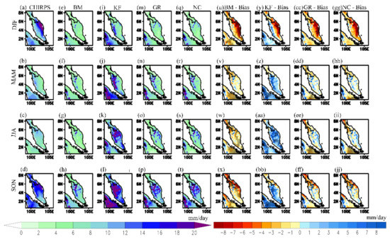
Figure 2.
Spatial patterns of precipitation for 2014–2018; (a–d) observation, (e–h) BM simulation, (i–l) KF simulation, (m–p) GR simulation, (q–t) NC simulation, (u–x) biased BM simulation, (y–bb) biased KF simulation, (cc–ff) biased GR simulation, and (gg–jj) biased NC simulation. From top to bottom, the rows represent the DJF, MAM, JJA, and SON seasons, respectively. The hatched area indicates significance at the 95% level. Units are in mm/day.
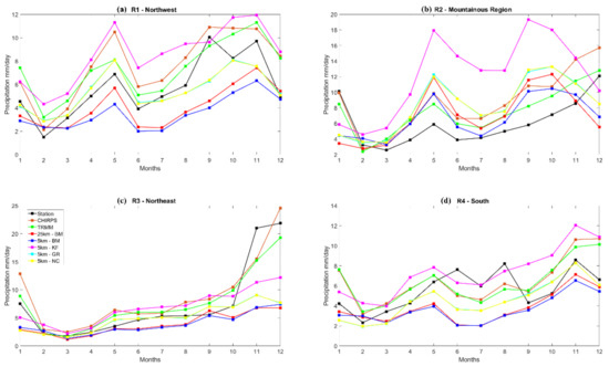
Figure 3.
Annual precipitation for four different regions over Peninsular Malaysia based on Figure 1 for different CPSs; (a) R1, (b) R2, (c) R3, and (d) R4. Units are in mm/day.
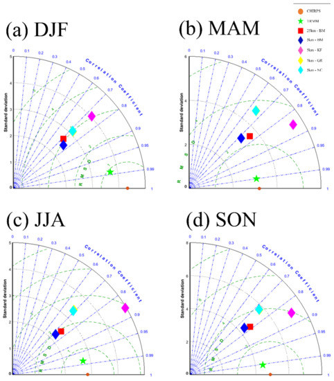
Figure 4.
Taylor diagram of precipitation over Peninsular Malaysia for the (a) DJF, (b) MAM, (c) JJA, and (d) SON seasons with different CPS simulations.
In Figure 2, the MAM season is shown on the second row, which consists of the results for CHIRPS: (b), BM (f), KF (j), GR (n), NC (r), BM-Bias (v), KF-Bias (z), GR-bias (dd), and NC-bias (hh). During the MAM season, there was an increase in precipitation which starts around early May, as shown in Figure 3. Generally, there were two peaks in which the precipitation was at its highest, which coincided with May and October or November and all the CPSs were able to simulate this. These patterns were even more prominent in the R2 region (Figure 3) where two distinct peaks are clearly shown. During this season, the KF scheme highlighted an absurd amount of over precipitation in the high altitude region (Figure 2p) where it had the highest bias, reaching 8 mm/day. The KF scheme had a very low performance relative to the other schemes. This is in line with the configuration of the KF scheme, which simulates high rainfall distributions even for dry season simulations [36,37,38]. This is consistent with the Taylor diagram results in Figure 4 where the KF scheme had the highest STD and RMSE among all CPSs especially during the MAM season. Despite that, KF schemes have a high correlation throughout the seasons. The KF scheme is presumed to have a high correlation because it has a better representation of extreme precipitation events, which is also the reason for the KF schemes to be used widely in typhoon simulations around Southeast Asia [6,39,40].
The JJA season in Figure 2 is shown on the third row, which consists of the results for CHIRPS: (c), BM (g), KF (k), GR (o), NC (s), BM-Bias (w), KF-Bias (aa), GR-Bias (ee), and NC-Bias (ii). During JJA, the BM scheme was capable of simulating the magnitude of precipitation derived from CHIRPS data quite well with biases of 1 to 2 mm/day, especially in the mountainous area of the Titiwangsa Range (Figure 2w). The other schemes tended to overestimate the rainfall magnitude. The capability of WRFs to function in complex terrains has always been a problem, as stated by Kong et al. [41], who noted a significant cold bias throughout the seasons in 15 km resolution simulations. In terms of cold biases, the KF scheme produced the worst results among all schemes as it heavily overestimated precipitation throughout the seasons. Figure 3 shows the annual cycle of precipitation for all CPSs in the four different regions shown in Figure 1. During JJA, which is supposed to be the driest season, all CPSs tended to simulate a higher amount of precipitation than gridded observational data from both CHIRPS and TRMM as well as station data, except for the BM scheme. During JJA, the BM scheme was the only scheme that produced a slight underestimation of precipitation intensity. These performances can be attributed to the conception of the BM scheme itself where temperature and moisture structure were independently constructed instead of being coupled in the same equation. An extensive study by Ratna et al. [36,42] also showed that the BM scheme is arguably the best scheme for simulating rainfall in tropical regions.
Overall, between all four choices of CPSs, none of them were able to simulate the effects of the northeast monsoon skillfully during DJF, which represents one of the most crucial seasons in Peninsular Malaysia, characterized by annual flooding and storms. The KF scheme, which supposedly tends to overestimate the amount of precipitation in tropical climates, was still unable to recreate the effects of the monsoon. The KF scheme had an overall poor performance across all seasons due to its overestimation of precipitation. Indeed, it is not designed for long precipitation simulations in the tropical area but is instead better suited for simulating storms and explicit events over small regions [25,43,44]. The performance of the NC run was below satisfactory as it produced little to no cumulus rain; this is understandable because the recommended resolution for using NC was at a 3 km resolution and above [28]. The results produced by the GR scheme were almost identical to those of the NC run, which indicated a lack of precipitation produced by the cumulus scheme. This problem stemmed from the small grid spacing, which the GR scheme could not handle due to the problem of idealized convection, as stated by Gilliland and Rowe [45], who also recommended a code modification to solve the underlying problem. The BM scheme proved to be the most reliable out of all of the CPSs, as supported by both Figure 2 and Figure 4. It has been consistently shown that the BM scheme is the most suitable for Southeast and East Asia [6,8,46]. Indeed, the BM scheme is favorable under tropical conditions due to the trigger function of the scheme, which is only triggered for surroundings with deep moisture. While this limitation is disadvantageous for environments dominated by arid conditions, the climate of Peninsular Malaysia is rarely arid as it is located at the equator and is consistently exposed to rain and sunlight.
3.2. Differential of Model Resolution Simulations
3.2.1. The Differences in 25 km and 5 km Simulations
For the second experiment, a higher resolution simulation was produced by downscaling the horizontal resolution of 25 km to 5 km with the same CPS, which is the BM scheme. The bias between the WRF simulation and CHIRPS observational data can be seen in row 1 (DJF) of Figure 5m,q. Both resolutions showed a high dry bias in the northeastern region of Peninsular Malaysia. This bias was present not only in this experiment, but also in other studies, such as those by Juneng et al. [7] and Salimun et al. [8]. Indeed, the monsoon arrives from the northeast of Peninsular Malaysia during the DJF seasons and is accompanied by a high amount of precipitation. A study by Raghavan et al. [47] covering the whole of Southeast Asia showed that none of the ten models studied produced satisfactory results, especially during the DJF and JJA seasons when the Peninsular Malaysia area showed a high dry bias. Ratna et al. [6] and Roux et al. [48] were also unable to simulate the expected amounts of precipitation during the DJF and SON seasons. Considering that this problem continues to persist in all models, by process of elimination, the models should not be the problem. Further work should investigate either the external forces that propagate the simulation or the physics involved in air–sea interactions. Additionally, Figure 5 depicts the precipitation patterns between the 25 and 5 km resolutions as being very similar and hard to differentiate, with a slight improvement of the rainfall features and intensity along the east coast of Peninsular Malaysia during DJF. Besides that, an enhancement of features in the mountain range was better depicted by the 5 km resolution simulation compared to that of the 25 km for all seasons. This shows that the 5 km simulation was able to better resolve the complex topography along the mountainous region compared to the 25 km resolution simulation. The results of this study are consistent with those of previous studies by Roux et al. [48] and Wang et al. [49]. Indeed, these authors also noted that the WRF has advantages for simulating mountainous areas as well as high altitude intermediate areas and sloping plains when using high-resolution simulations.
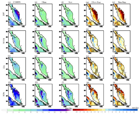
Figure 5.
Spatial pattern of precipitation for the year 2014–2018; (a–d) observation, (e–h) 25 km simulation, (i–l) 5 km simulation, (m–p) biased 25 km simulation, and (q–t) biased 5 km simulation. From top to bottom, the rows represent the season of DJF, MAM, JJA, and SON seasons, respectively. Both 25 km and 5 km are using BM schemes. The hatched area indicates significance at the 95% level. Units are in mm/day.
Figure 6a–d depicts the annual precipitation patterns in four different regions of Peninsular Malaysia from R1 to R4, respectively. Region R1 covers the west of Peninsular Malaysia, R2 covers the center of Peninsular Malaysia, R3 covers the west coast of Peninsular Malaysia, and R4 covers the south of Peninsular Malaysia. These four regions have different annual spatial precipitation patterns due to the monsoons and the position of the Titiwangsa Range in the center of Peninsular Malaysia affecting the wind patterns covering the whole of Peninsular Malaysia [50,51,52]. Observational data from CHIRPS, TRMM, and the stations were used as references. Both CHIRPS and TRMM conformed to the annual spatial patterns obtained from the station data. According to Figure 6, the models performed better when simulating the precipitation patterns in R1 (Figure 6a) and R4 (Figure 6d) than in R2 (Figure 6b) and R3 (Figure 6c). One of the reasons for this would be the topography of these four areas. R1 and R4 cover areas with a relatively simple topography, which only experience a few prominent climate events that heavily impact the yearly amount of precipitation. On the other hand, R2 consists of a high altitude region extending from the border with Thailand southward towards the center of Peninsular Malaysia. In general, WRF climate models tend to generate higher amounts of precipitation in high altitude regions, hence the over precipitation shown throughout the R2 region. Regardless, among all regions, R2 exhibited the most improvement between the 25 km and 5 km simulations with the 5 km simulation showing a better performance because WRF generally have better performances in high altitude regions if a high resolution is used. Distinct changes in precipitation patterns were seen in previous studies [53,54] when resolutions of 9 km and higher were used. In the case of Figure 6c, region R3 was heavily impacted by the northeast monsoon, which is accompanied by heavy precipitation from November until January. As shown in Figure 6c, both the 5 and 25 km models were able to simulate the precipitation patterns closely with the observational data until October but they could not replicate the spike in precipitation intensity from November onwards, replicating the same spatial pattern as the DJF season in Figure 5b,c. This follows the same pattern as that of studies conducted by Juneng et al. [7] and Ratna et al. [6] where the precipitation intensities in the northeast region of Peninsular Malaysia (R3) were lower than expected from November until January. There is a high probability that the cause was the inability of the RCM to simulate the effects of the northeast monsoon. It is still debatable whether the problem was the air–sea interaction of the RCM model that generalizes the air–sea mixing on the surface or whether the problem stemmed from the low-resolution climate data that was provided by the GCM. Further experiments are needed to rectify the problem by focusing on simulating a proper northeast monsoon movement.
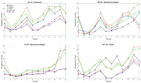
Figure 6.
Annual precipitation for four different regions over Peninsular Malaysia based on Figure 1; (a) R1, (b) R2, (c) R3, and (d) R4. Units are in mm/day. Both 25 km and 5 km are using BM schemes.
As supporting evidence, further analyses was conducted using Taylor diagrams to evaluate the COR, RMSE, and STD of both the 5 and 25 km simulations. As shown in Figure 7, the 5 km simulation exhibited a slight improvement consistently during all four seasons, in contrast to the 25 km simulation. Still, the differences between these two models were not significant enough to warrant a comparison between the use of higher resolution simulations for climate studies. Considering the results from Figure 5, Figure 6 and Figure 7, a notable improvement of the 5 km run was shown in two categories: spatial precipitation pattern in the Northeast Peninsular region during DJF season and the annual precipitation in the R2 region. During DJF, dry biases along the northeast of Peninsular Malaysia are significantly less in the 5 km run as compared to the 25 km. In Figure 3, 5 km consistently follows the intensity of precipitation in the R2 region compared to 25 km, especially during May and October. Twenty-five km runs have a tendency to overestimate the amount of precipitation during these two months. This shows that 5 km has a significant improvement in the high altitude region of Peninsular Malaysia. As a reference, this experiment only considered resolution as the variable and the other setting remained constant. It is generally accepted that an increase in horizontal and vertical resolution would further improve the results of the reanalysis. However, according to a study by Demory et al. [55], an increase in resolution does not simply have a linear positive effect on precipitation. Precipitation over the ocean will decrease, while that over land will increase in intensity. This is due to the partitioning of moisture fluxes falling more towards non-local moisture than local circulation. Hence, a change in the resolution without any changes to the physics that regulate the ocean to air interactions will not significantly improve the results.
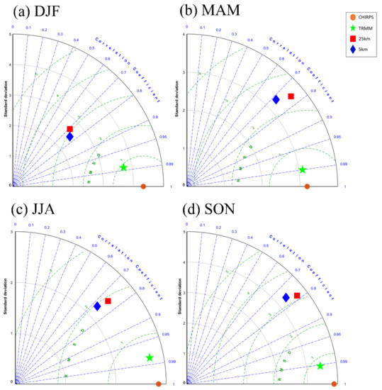
Figure 7.
Taylor diagram of precipitation over Peninsular Malaysia for the (a) DJF, (b) MAM, (c) JJA, and (d) SON seasons. Both 25 km and 5 km are using BM schemes.
3.2.2. Added Value of Using Higher Resolution Simulations
A simulation with a resolution of 1.6 km (D03) was used as a higher resolution simulation for the WRF model from the parent domain of 5 km (D02) because the 3:1 ratio is preferable in the dynamical downscaling of WRFs. The grid of the WRF was constructed using an Arakawa-C grid, which has a better interpolation accuracy and efficiency if a ratio of 3:1 is used [56]. A high-resolution simulation was used because Peninsular Malaysia covers an area of roughly 131,732 km2 with complex mountainous terrain at the center of it. Thus, a high resolution is needed to depict the local anomalies and convection that occur in the area. An investigation of the diurnal cycles in Peninsular Malaysia is further required to provide a better understanding of the simulation of rainfall. Indeed, a good depiction and representation of a diurnal cycle is one of the most important results that gauge the performance of an atmospheric model, especially in tropical regions [57]. Figure 8, Figure 9, Figure 10 and Figure 11 shows the mean diurnal cycle in regions R1, R2, R3, and R4, respectively. According to Figure 8, both the 25 and 5 km resolutions tended to create lower hourly precipitation in the morning, but the 1.6 km simulation was able to produce the same precipitation pattern as the observation, especially in Setiawan (d), Alor Setar (e), and Butterworth (f). From Figure 9, in the mountainous region of R2, the 1.6 km simulation fared much better than the other models, especially in the morning. In terms of rainfall patterns, the 1.6 km resolution was once again able to most closely follow the erratic increase of precipitation, while both the 25 and 5 km simulations tended to underestimate the amount of precipitation from morning until noon before peaking in the evening. This precipitation pattern was the same throughout all regions, and all stations showed an increase in precipitation during 1600 LST; according to Oki et al. [58], these peaks are evidence of the thermodynamic forces affecting the convective rainfall in the evenings. This is consistent with findings from Oki et al. [58] who observed the same pattern. This will cause large STD during the afternoon/evening due to seasonal effects during the intermonsoon season of MAM and SON. Thus, a high amount of STD during the afternoon/evening can be observed (figure not shown). If error bars are included, clear information cannot be captured. In both R2 and R3 regions in Figure 9 and Figure 10, precipitation was expected to peak higher than in other regions and all three simulations followed the same pattern. However, all simulations tended to peak early while the observational data showed the peak occurring a lot later and higher. Figure 10 shows the diurnal cycles in the R3 region, which is heavily influenced by the northeast monsoon during the DJF season. In both Figure 2 and Figure 5, the DJF season exhibited the highest precipitation bias for both the 25 and 5 km resolutions, while tending to underestimate the amount of precipitation in the northeastern part of Peninsular Malaysia. The diurnal cycle for both 25 km and 5 km simulations again showed the same pattern of underestimation with a low precipitation intensity. The 1.6 km simulation, on the other hand, was able to simulate the diurnal cycle with a much closer intensity to that of the observational data and fared much better than the 25 and 5 km runs. Figure 11 yields one of the most interesting results. In the southern part of Peninsular Malaysia, R4 exhibited three obvious peaks in almost all the stations during 700 LST, 900 LST, and 1900 LST. Both the 25 and 5 km simulations were unable to pick up the first two signals in the morning and peaked early for the third signal. On the other hand, the 1.6 km simulation was able to pick up on all three signals with varying intensities. In all simulations, all models were able to simulate the precipitation trends and patterns with a high accuracy but had difficulty simulating the precipitation spike in the evening. The 25 km model tended to overestimate the amount of precipitation, especially in the early morning and during the evening precipitation. There is a noticeable lag in peaks in all three models consistently during the evening for almost all stations, which suggests that the precipitation during the morning did not dissipate quickly enough [59]. The 5 km simulation also tended to underestimate the precipitation most of the time and in some cases was unable to simulate the sudden increase in precipitation during the evening. If the simulation was able to pick up the signal to increase the precipitation, it tended to overestimate greatly. In all four regions, the 1.6 km resolution was shown to have significant added value in regions where extreme climate is combined with a difficult topography. The 1.6 km simulation was also better able to simulate a higher precipitation intensity during the morning than the 25 and 5 km simulations. However, the 1.6 km resolution tended to overestimate the amount of precipitation and exhibit erratic rainfall patterns. Another issue that is visible in all three models was the inability to pick up a second signal of the precipitation spike after the initial spike at 1600 LST. This was not exclusive to WRFs, as models such as the NHRCM are characterized by suppressed diurnal precipitation [52,60]. All three simulations relaxed and always showed a downward trend after the initial spike. While this was the usual trend, in some places in the R2 region, they tended to exhibit another spike in precipitation after the initial one at 1600 LST and all three models continued to show a downward trend despite the station data showing otherwise.
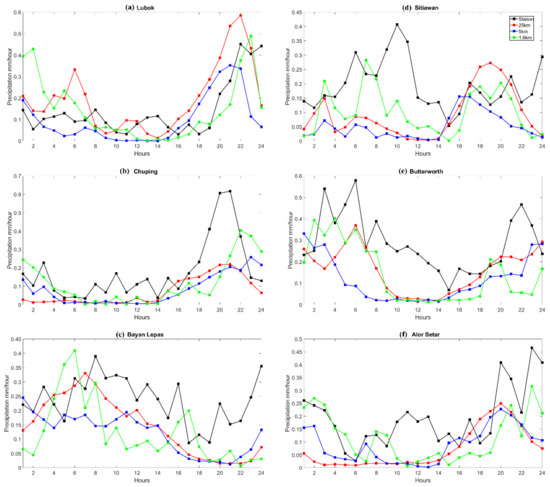
Figure 8.
Diurnal cycles for all station data for 1 year (2013) in region 1 of Peninsular Malaysia; (a) Lubok, (b) Chuping, (c) Bayan Lepas, (d) Sitiawan, (e) Butterworth, and (f) Alor Setar. Units are in mm/hour.
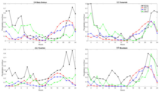
Figure 9.
Diurnal cycles for all station data for 1 year (2013) in region 2 of Peninsular Malaysia; (a) Batu Embun, (b) Kuantan, (c) Temerloh, and (d) Muadzam. Units are in mm/hour.
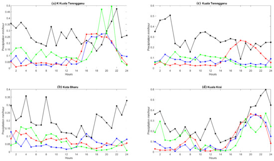
Figure 10.
Diurnal cycles for all station data for 1 year (2013) in region 3 of Peninsular Malaysia; (a) K. Kuala Terengganu, (b) Kota Bharu, (c) Kuala Terengganu, and (d) Kuala Krai. Units are in mm/hour.
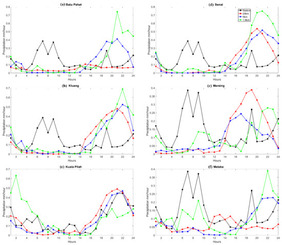
Figure 11.
Diurnal cycles for all station data for 1 year (2013) in region 4 of Peninsular Malaysia; (a) Batu Pahat, (b) Kluang, (c) Kuala Pilah, (d) Senai, (e) Mersing, and (f) Melaka. Units are in mm/hour.
Despite the increase in resolution for both the 25 and 5 km simulations, the differences were not significant. This was simply due to the differences between the 25 and 5 km simulations, as shown in Figure 7 where there are only marginal differences in the results of the Taylor diagram despite the 5 km model performing better. The probable cause for this was the difference between seasonality and the diurnal cycle which, in terms of time variability, was a huge difference. In this diurnal analysis, we could conclude that there were two factors that contributed to the lack of accuracy of the WRF model in simulating precipitation in Malaysia. The first event was the peak during the evening and the second event was the underestimation of precipitation during the morning. This problem occurred consistently in all regions and all simulations had difficulties in simulating the erratic nature of the evening precipitation. Auriol et al. [61] concluded that a resolution of 4 km or higher is needed for a better precipitation simulation on a convection-permitting scale. However, according to Jeworrek et al. [28], as the resolution reaches the gray zone (around 1–4 km), several precautions must be heeded. One of them is the noise that could build up into major errors. It has been stated that formally deterministic fluid systems will have an observational error that acts as noise at first but eventually decreases the capability of the precipitation simulation due to an effect called double penalty [62,63]. This is because the error might have originated from the input of the coarser domain, which has a low resolution or the usage of the same scheme with a different resolution. The nature of a nested simulation relies too much on the initial boundary conditions of a coarser input and, in hindsight, it is advisable that upon nesting at a higher resolution, each resolution must be configured to their highest performance. In this experiment, we already saw the stark differences a CPS alone could produce in a precipitation profile at a 5 km resolution. There is a myriad of settings and configurations that should be considered in further studies before proceeding towards a finer resolution and the results of this experiment support this. Another problem is that a 5 km resolution is not high enough to simulate diurnal precipitation. The area of Peninsular Malaysia is small, surrounded by water bodies, and has a complex topography which renders simulations by RCMs extremely difficult. In this study, we found that further increasing the resolution to 1.6 km resulted in a significant increase in added value as it allowed a higher precipitation intensity to be simulated in the morning in all four regions; in Figure 11, which shows the results for region R4, only the 1.6 km simulation was able to pick up the three peak signals present in the observations.
4. Conclusions
This experiment was designed to investigate the impact of CPSs and the importance of high-resolution precipitation simulations using the WRF model. The 25, 5, and 1.6 km horizontal resolutions used by Ratna et al. [6] were implemented as a template while keeping the other variables except for CPS constant, yielding insightful results.
For the first study, the CPS comparison for the 5 km resolution model showed the BM scheme as the best among the other CPSs investigated in the study. The GR scheme produced rainfall distribution results that were similar to those of the NC run. Indeed, the GR scheme could be problematic as it tended to turn off the simulation of cumulus cloud formation and, thus, both CPSs simulated lower rainfall distribution than the other CPSs. The KF scheme tended to produce high rainfall distributions relative to the other schemes, especially in region R2 and in high altitude areas. However, it had a good performance in simulating the effects of the northeast monsoon compared to other CPSs. Overall, the BM scheme had the best performance in simulating rainfall distributions in Peninsular Malaysia, consistent with other studies conducted in the tropics. In nested model simulations, the model tended to have a better performance if the same settings were used. This could explain the marginal differences in the performance of the 5 and 25 km simulations considered in this study.
A comparison between the 25 and 5 km simulations showed an improvement in the use of higher resolutions. However, during the DJF season, the eastern region of Peninsular Malaysia exhibited a high bias due to high rainfall distributions generated by the northeast monsoon phenomenon. Both resolutions were unable to simulate the high rainfall distribution in the eastern part of Peninsular Malaysia. Indeed, the northeast monsoon is difficult to simulate well and other models such as RegCM4 and MM5 have a similar problem simulating the intensity of rainfall in the northeast of Peninsular Malaysia during DJF. Overall, although the 5 km simulation had a better performance than the 25 km one, the differences between the two models were not significant.
Further investigation at higher resolutions using 1.6 km simulations led to a significant increase in added value as these were able to simulate a higher precipitation intensity in the morning in all four regions compared to the results of the 25 and 5 km simulations. The 1.6 km simulation had the only resolution that was able to pick up the three peak signals present in the observations. This indicates that the 1.6 km resolution could effectively resolve atmospheric convection even when CPSs were not used. This also implies that resolution had a significant influence on the model performances and that 5 km was not a high enough resolution. However, further studies are required to determine the best configuration for higher resolution simulations as many factors must be considered to minimize the errors. The atmospheric configuration for this experiment was quite challenging as the northeast monsoon is a complex feature which many models have consistently failed to simulate skillfully. Atmospheric thermodynamics have always been an integral part of understanding cloud microphysics and convection parameterization. Hence, future studies on air−sea interactions are suggested to further investigate the cause of this phenomenon.
Author Contributions
E.S., F.T. and L.J. designed the study. E.S., M.Z. and A.A.A. analyzed the data and led the writing of the manuscript. A.A.A. and M.S.F.M. conducted the simulation at the 25 and 5 km resolutions using NAHRIM’s HPC, and A.A.A. and J.X.C. conducted the simulation at 1.6 km using UMT’s HPC. All the authors contributed to the writing and data interpretation. All authors have read and agreed to the published version of the manuscript.
Funding
This research was funded by the Universiti Kebangsaan Malaysia, grant number GGPM-2018-068 and the Ministry of Education Malaysia, grant number FRGS/1/2017/WAB05/UKM/01/2 and the Faculty of Science and Technology, Universiti Kebangsaan Malaysia under the grant number PP-FST-2022.
Institutional Review Board Statement
Not applicable.
Informed Consent Statement
Not applicable.
Acknowledgments
We appreciate the assistance in facilitating the study that HPC simulations from NAHRIM and Universiti Malaysia Terengganu provided.
Conflicts of Interest
The authors declare no conflict of interest.
References
- Phillips, N.A. The general circulation of the atmosphere: A numerical experiment. Q. J. R. Meteorol. Soc. 1956, 82, 123–164. [Google Scholar] [CrossRef]
- Giorgi, F.; Bates, G.T. The climatological skill of a regional model over complex terrain. Mon. Weather. Rev. 1989, 117, 2325–2347. [Google Scholar] [CrossRef]
- Giorgi, F. Simulation of regional climate using a limited area model nested in a general circulation model. J. Clim. 1990, 3, 941–963. [Google Scholar] [CrossRef]
- Arakawa, A. Modelling clouds and cloud processes for use in climate models. In The Physical Basis of Climate and Climate Modelling; SEE N 76-19675 10-47; WMO: Geneva, Switzerland, 1975; pp. 187–197. [Google Scholar]
- Peña-Arancibia, J.L.; Van Dijk, A.I.; Renzullo, L.J.; Mulligan, M. Evaluation of precipitation estimation accuracy in reanalyses, satellite products, and an ensemble method for regions in Australia and South and East Asia. J. Hydrometeorol. 2013, 14, 1323–1333. [Google Scholar] [CrossRef]
- Ratna, S.B.; Ratnam, J.; Behera, S.; Tangang, F.T.; Yamagata, T. Validation of the WRF regional climate model over the subregions of Southeast Asia: Climatology and interannual variability. Clim. Res. 2017, 71, 263–280. [Google Scholar] [CrossRef][Green Version]
- Juneng, L.; Tangang, F.; Chung, J.X.; Ngai, S.T.; Tay, T.W.; Narisma, G.; Cruz, F.; Phan-Van, T.; Ngo-Duc, T.; Santisirisomboon, J. Sensitivity of Southeast Asia rainfall simulations to cumulus and air-sea flux parameterizations in RegCM4. Clim. Res. 2016, 69, 59–77. [Google Scholar] [CrossRef]
- Salimun, E.; Tangang, F.; Juneng, L. Simulation of heavy precipitation episode over eastern Peninsular Malaysia using MM5: Sensitivity to cumulus parameterization schemes. Meteorol. Atmos. Phys. 2010, 107, 33–49. [Google Scholar] [CrossRef]
- Zhang, W.; Wang, Y.; Jin, F.F.; Stuecker, M.F.; Turner, A.G. Impact of different El Niño types on the El Niño/IOD relationship. Geophys. Res. Lett. 2015, 42, 8570–8576. [Google Scholar] [CrossRef]
- Wyngaard, J.C. Toward numerical modeling in the “Terra Incognita”. J. Atmos. Sci. 2004, 61, 1816–1826. [Google Scholar] [CrossRef]
- Gerard, L. An integrated package for subgrid convection, clouds and precipitation compatible with meso-gamma scales. Q. J. R. Meteorol. Soc. A J. Atmos. Sci. Appl. Meteorol. Phys. Oceanogr. 2007, 133, 711–730. [Google Scholar] [CrossRef]
- Kealy, J.C.; Efstathiou, G.A.; Beare, R.J. The onset of resolved boundary-layer turbulence at grey-zone resolutions. Bound. Layer Meteorol. 2019, 171, 31–52. [Google Scholar] [CrossRef]
- Schwartz, C.S.; Kain, J.S.; Weiss, S.J.; Xue, M.; Bright, D.R.; Kong, F.; Thomas, K.W.; Levit, J.J.; Coniglio, M.C. Next-day convection-allowing WRF model guidance: A second look at 2-km versus 4-km grid spacing. Mon. Weather. Rev. 2009, 137, 3351–3372. [Google Scholar] [CrossRef]
- Kain, J.S.; Weiss, S.J.; Bright, D.R.; Baldwin, M.E.; Levit, J.J.; Carbin, G.W.; Schwartz, C.S.; Weisman, M.L.; Droegemeier, K.K.; Weber, D.B. Some practical considerations regarding horizontal resolution in the first generation of operational convection-allowing NWP. Weather. Forecast. 2008, 23, 931–952. [Google Scholar] [CrossRef]
- Field, P.R.; Brožková, R.; Chen, M.; Dudhia, J.; Lac, C.; Hara, T.; Honnert, R.; Olson, J.; Siebesma, P.; de Roode, S. Exploring the convective grey zone with regional simulations of a cold air outbreak. Q. J. R. Meteorol. Soc. 2017, 143, 2537–2555. [Google Scholar] [CrossRef]
- Petch, J.; Brown, A.; Gray, M. The impact of horizontal resolution on the simulations of convective development over land. Q. J. R. Meteorol. Soc. A J. Atmos. Sci. Appl. Meteorol. Phys. Oceanogr. 2002, 128, 2031–2044. [Google Scholar] [CrossRef]
- Bryan, G.H.; Wyngaard, J.C.; Fritsch, J.M. Resolution requirements for the simulation of deep moist convection. Mon. Weather. Rev. 2003, 131, 2394–2416. [Google Scholar] [CrossRef]
- Holloway, C.E. Convective aggregation in realistic convective-scale simulations. J. Adv. Modeling Earth Syst. 2017, 9, 1450–1472. [Google Scholar] [CrossRef]
- Sakradzija, M.; Seifert, A.; Dipankar, A. A stochastic scale-aware parameterization of shallow cumulus convection across the convective gray zone. J. Adv. Modeling Earth Syst. 2016, 8, 786–812. [Google Scholar] [CrossRef]
- Arakawa, A.; Chen, J.-M. Closure assumptions in the cumulus parameterization problem. J. Meteorol. Soc. Jpn. Ser. II 1986, 64, 107–131. [Google Scholar] [CrossRef]
- Hammarstrand, U. Questions involving the use of traditional convection parameterization in NWP models with a higher resolution. Tellus A Dyn. Meteorol. Oceanogr. 1998, 50, 265–282. [Google Scholar] [CrossRef]
- Deng, A.; Stauffer, D.R. On improving 4-km mesoscale model simulations. J. Appl. Meteorol. Climatol. 2006, 45, 361–381. [Google Scholar] [CrossRef]
- Kotroni, V.; Lagouvardos, K. Evaluation of MM5 high-resolution real-time forecasts over the urban area of Athens, Greece. J. Appl. Meteorol. 2004, 43, 1666–1678. [Google Scholar] [CrossRef]
- Skamarock, W.; Klemp, J.; Dudhia, J.; Gill, D.; Barker, D.G.; Duda, M.; Huang, X.-Y.; Wang, W.; Powers, J.G. A Description of the Advanced Research WRF Version 3; NCAR Technical Note; National Center for Atmospheric Research (NCAR)/TN-475+ STR, NCAR: Boulder, CO, USA, 2008. [Google Scholar]
- Kain, J.S. The Kain–Fritsch convective parameterization: An update. J. Appl. Meteorol. 2004, 43, 170–181. [Google Scholar] [CrossRef]
- Janjić, Z.I. The step-mountain eta coordinate model: Further developments of the convection, viscous sublayer, and turbulence closure schemes. Mon. Weather. Rev. 1994, 122, 927–945. [Google Scholar] [CrossRef]
- Grell, G.A. A Description of the Fifth-Generation Penn State/NCAR Mesoscale Model (MM5); Technical NoteNCAR/TN-398+ STR; National Center for Atmospheric Research (NCAR): Boulder, SO, USA, 1995. [Google Scholar]
- Jeworrek, J.; West, G.; Stull, R. Evaluation of cumulus and microphysics parameterizations in WRF across the convective gray zone. Weather. Forecast. 2019, 34, 1097–1115. [Google Scholar] [CrossRef]
- Juneng, L.; Tangang, F.T. Evolution of ENSO-related rainfall anomalies in Southeast Asia region and its relationship with atmosphere–ocean variations in Indo-Pacific sector. Clim. Dyn. 2005, 25, 337–350. [Google Scholar] [CrossRef]
- Amirudin, A.A.; Salimun, E.; Tangang, F.; Juneng, L.; Zuhairi, M. Differential influences of teleconnections from the Indian and Pacific Oceans on rainfall variability in Southeast Asia. Atmosphere 2020, 11, 886. [Google Scholar] [CrossRef]
- Lim, S.Y.; Marzin, C.; Xavier, P.; Chang, C.-P.; Timbal, B. Impacts of boreal winter monsoon cold surges and the interaction with MJO on Southeast Asia rainfall. J. Clim. 2017, 30, 4267–4281. [Google Scholar] [CrossRef]
- Ayoub, A.B.; Tangang, F.; Juneng, L.; Tan, M.L.; Chung, J.X. Evaluation of gridded precipitation datasets in Malaysia. Remote Sens. 2020, 12, 613. [Google Scholar] [CrossRef]
- Wagner, A.; Heinzeller, D.; Wagner, S.; Rummler, T.; Kunstmann, H. Explicit convection and scale-aware cumulus parameterizations: High-resolution simulations over areas of different topography in Germany. Mon. Weather. Rev. 2018, 146, 1925–1944. [Google Scholar] [CrossRef]
- Li, X.; Xie, S.-P.; Gille, S.T.; Yoo, C. Atlantic-induced pan-tropical climate change over the past three decades. Nat. Clim. Chang. 2016, 6, 275–279. [Google Scholar] [CrossRef]
- Ngo-Duc, T.; Tangang, F.T.; Santisirisomboon, J.; Cruz, F.; Trinh-Tuan, L.; Nguyen-Xuan, T.; Phan-Van, T.; Juneng, L.; Narisma, G.; Singhruck, P. Performance evaluation of RegCM4 in simulating extreme rainfall and temperature indices over the CORDEX-Southeast Asia region. Int. J. Climatol. 2017, 37, 1634–1647. [Google Scholar] [CrossRef]
- Ratna, S.B.; Ratnam, J.; Behera, S.; Rautenbach, C.d.; Ndarana, T.; Takahashi, K.; Yamagata, T. Performance assessment of three convective parameterization schemes in WRF for downscaling summer rainfall over South Africa. Clim. Dyn. 2014, 42, 2931–2953. [Google Scholar] [CrossRef]
- Huang, D.; Gao, S. Impact of different cumulus convective parameterization schemes on the simulation of precipitation over China. Tellus A Dyn. Meteorol. Oceanogr. 2017, 69, 1406264. [Google Scholar] [CrossRef]
- Otieno, G.; Mutemi, J.; Opijah, F.; Ogallo, L.; Omondi, M. The sensitivity of rainfall characteristics to cumulus parameterization schemes from a WRF model. Part I: A case study over East Africa during wet years. Pure Appl. Geophys. 2020, 177, 1095–1110. [Google Scholar] [CrossRef]
- Raktham, C.; Bruyère, C.; Kreasuwun, J.; Done, J.; Thongbai, C.; Promnopas, W. Simulation sensitivities of the major weather regimes of the Southeast Asia region. Clim. Dyn. 2015, 44, 1403–1417. [Google Scholar] [CrossRef]
- Huo, Y.; Peltier, W.R. The southeast asian monsoon: Dynamically downscaled climate change projections and high resolution regional ocean modelling on the effects of the Tibetan Plateau. Clim. Dyn. 2021, 56, 2597–2616. [Google Scholar] [CrossRef]
- Kong, S.S.-K.; Sentian, J.; Bidin, K. Evaluation of Weather Research Forecast (WRF) modeling system on surface temperature and precipitation over Malaysia region. Adv. Nat. Appl. Sci. 2015, 9, 20–25. [Google Scholar]
- Ratna, S.B.; Osborn, T.; Joshi, M.M. Multidecadal climate variability of East Asia during the last millennium: Roles of external forcing and internal variability. In Proceedings of the AGU Fall Meeting Abstracts, Washington, DC, USA, 10–14 December 2018; p. PP43C-1942. [Google Scholar]
- Cruz, F.T.; Sasaki, H.; Narisma, G.T. Assessing the sensitivity of the non-hydrostatic regional climate model to boundary conditions and convective schemes over the Philippines. J. Meteorol. Soc. Jpn. Ser. II 2016, 94, 165–179. [Google Scholar] [CrossRef]
- Shepherd, T.J.; Walsh, K.J. Sensitivity of hurricane track to cumulus parameterization schemes in the WRF model for three intense tropical cyclones: Impact of convective asymmetry. Meteorol. Atmos. Phys. 2017, 129, 345–374. [Google Scholar] [CrossRef]
- Gilliland, E.K.; Rowe, C.M. A comparison of cumulus parameterization schemes in the WRF model. In Proceedings of the 87th AMS Annual Meeting & 21th Conference on Hydrology, San Antonio, TX, USA, 13–18 January 2007. [Google Scholar]
- Pan, H.-l.; Wu, W.-S. Implementing a mass flux convection parameterization package for the NMC medium-range forecast model. NMC Off. Note 1995, 409. [Google Scholar]
- Raghavan, S.V.; Liu, J.; Nguyen, N.S.; Vu, M.T.; Liong, S.-Y. Assessment of CMIP5 historical simulations of rainfall over Southeast Asia. Theor. Appl. Climatol. 2018, 132, 989–1002. [Google Scholar] [CrossRef]
- Roux, G.; Liu, Y.; Monache, L.; Sheu, R.-S.; Warner, T.T. Verification of high resolution WRF-RTFDDA surface forecasts over mountains and plains. In Proceedings of the 10th WRF Users’ Workshop, Boulder, CO, USA, 23–26 June 2009; pp. 20–23. [Google Scholar]
- Wang, G.; Cai, W. Two-year consecutive concurrences of positive Indian Ocean Dipole and Central Pacific El Niño preconditioned the 2019/2020 Australian “black summer” bushfires. Geosci. Lett. 2020, 7, 19. [Google Scholar] [CrossRef]
- Suhaila, J.; Deni, S.M.; Zin, W.W.; Jemain, A.A. Trends in peninsular Malaysia rainfall data during the southwest monsoon and northeast monsoon seasons: 1975–2004. Sains Malays. 2010, 39, 533–542. [Google Scholar]
- Loo, Y.Y.; Billa, L.; Singh, A. Effect of climate change on seasonal monsoon in Asia and its impact on the variability of monsoon rainfall in Southeast Asia. Geosci. Front. 2015, 6, 817–823. [Google Scholar] [CrossRef]
- Jamaluddin, A.F.; Tangang, F.; Chung, J.X.; Juneng, L.; Sasaki, H.; Takayabu, I. Investigating the mechanisms of diurnal rainfall variability over Peninsular Malaysia using the non-hydrostatic regional climate model. Meteorol. Atmos. Phys. 2018, 130, 611–633. [Google Scholar] [CrossRef]
- Yáñez-Morroni, G.; Gironás, J.; Caneo, M.; Delgado, R.; Garreaud, R. Using the weather research and forecasting (WRF) model for precipitation forecasting in an Andean region with complex topography. Atmosphere 2018, 9, 304. [Google Scholar] [CrossRef]
- Schumacher, V.; Fernández, A.; Justino, F.; Comin, A. WRF high resolution dynamical downscaling of precipitation for the Central Andes of Chile and Argentina. Front. Earth Sci. 2020, 8, 1–19. [Google Scholar] [CrossRef]
- Demory, M.-E.; Vidale, P.L.; Roberts, M.J.; Berrisford, P.; Strachan, J.; Schiemann, R.; Mizielinski, M.S. The role of horizontal resolution in simulating drivers of the global hydrological cycle. Clim. Dyn. 2014, 42, 2201–2225. [Google Scholar] [CrossRef]
- Mesinger, F.; Arakawa, A. Numerical Methods Used in Atmospheric Models; Global Atmospheric Research Programme (GARP), WMO-ICSU Joint Scientific Committee: Geneva, Switzerland, 1976; Volume 1. [Google Scholar]
- Bhatt, B.C.; Sobolowski, S.; Higuchi, A. Simulation of diurnal rainfall variability over the Maritime Continent with a high-resolution regional climate model. J. Meteorol. Soc. Jpn. Ser. II 2016, 94, 89–103. [Google Scholar] [CrossRef][Green Version]
- Oki, T.; Musiake, K. Seasonal change of the diurnal cycle of precipitation over Japan and Malaysia. J. Appl. Meteorol. Climatol. 1994, 33, 1445–1463. [Google Scholar] [CrossRef]
- Goines, D.; Kennedy, A. Precipitation From a Multiyear Database of Convection-Allowing WRF Simulations. J. Geophys. Res. Atmos. 2018, 123, 2424–2453. [Google Scholar] [CrossRef]
- Lim, J.T. Characteristics of the Winter Monsoon over the Malaysian Region; University of Hawai’i at Manoa: Ann Arbor, MI, USA, 1979. [Google Scholar]
- Auriol, F.; Gayet, J.-F.; Febvre, G.; Jourdan, O.; Labonnote, L.; Brogniez, G. In situ observation of cirrus scattering phase functions with 22 and 46 halos: Cloud field study on 19 February 1998. J. Atmos. Sci. 2001, 58, 3376–3390. [Google Scholar] [CrossRef]
- Lorenz, E.N. The predictability of a flow which possesses many scales of motion. Tellus 1969, 21, 289–307. [Google Scholar] [CrossRef]
- Clark, A.J.; Gallus, W.A., Jr.; Xue, M.; Kong, F. A comparison of precipitation forecast skill between small convection-allowing and large convection-parameterizing ensembles. Weather. Forecast. 2009, 24, 1121–1140. [Google Scholar] [CrossRef]


Publisher’s Note: MDPI stays neutral with regard to jurisdictional claims in published maps and institutional affiliations. |
© 2022 by the authors. Licensee MDPI, Basel, Switzerland. This article is an open access article distributed under the terms and conditions of the Creative Commons Attribution (CC BY) license (https://creativecommons.org/licenses/by/4.0/).