Abstract
One of the well-known challenges of fog forecasting is the high spatio-temporal variability of fog. An ensemble forecast aims to capture this variability by representing the uncertainty in the initial/lateral boundary conditions (ICs/BCs) and model physics. The present study highlights a new operational Ensemble Forecast System (EFS) developed by the Indian Institute of Tropical Meteorology (IITM), Pune, to predict the fog over the Indo-Gangetic Plain (IGP) region using the visibility (Vis) diagnostic algorithm. The EFS framework comprises the WRF model with a 4 km horizontal resolution, initialized by 21 ICs/BCs. The advantages of probabilistic fog forecasting have been demonstrated by comparing control (CNTL) and ensemble-based fog forecasts. The forecast is verified using fog observations from the Indira Gandhi International (IGI) airport during the winter months of 2020–2021 and 2021–2022. The results show that with a probability threshold of 50%, the ensemble forecasts perform better than the CNTL forecasts. The skill scores of EFS are relatively promising, with a Hit Rate of 0.95 and a Critical Success Index of 0.55; additionally, the False Alarm Rate and Missing Rate are low, with values of 0.43 and 0.04, respectively. The EFS could correctly predict more fog events (37 out of 39) compared with the CNTL forecast (31 out of 39) and shows the potential skill. Furthermore, EFS has a substantially reduced error in predicting fog onset and dissipation (mean onset and dissipation error of 1 h each) compared to the CNTL forecasts.
1. Introduction
For the past three decades, it has been observed that the reduced visibility during dense fog episodes severely affects the rail–road–air transport systems and leads to economic losses and life-threatening hazards in the Indo-Gangetic Plain (IGP) region [1,2,3,4]. Moreover, the reduction in insolation during foggy conditions has substantially fluctuated the power output of solar power plants over the different parts of North India in recent years. Better forecasts of fog would help to mitigate such economic losses and minimize the possible damage to life and property.
Through state-of-the-art numerical models and statistical approaches such as a decision tree [5,6,7], neural network [8,9], fuzzy logic [10,11], and artificial intelligence/machine learning [12,13,14,15], the predictability of fog could be enhanced by reproducing the fog-relevant thermodynamical state of the atmosphere. Although the nowcasting (6–12 h) skill of statistical approaches for site-specific fog is reasonably satisfactory, these approaches have limited spatial resolution and depend on long-term fog field observations. The progress in the numerical prediction of fog has a long history of 40–50 years. The improvements in the numerical weather prediction (NWP) models in terms of vertical/horizontal resolutions [16,17,18], physical parameterization schemes [19,20,21], and land surface processes [22,23,24] have been possible due to the support of extensive fog field observations from across the globe [4,25,26,27,28,29]. Several research centers have evaluated the performance of the NWP models and attempted to operationalize them for short-range (12–72 h) fog prediction on the local to regional scale [30,31,32,33,34]. Although the NWP models have made significant progress, the spatiotemporal variability of fog poses a major problem for forecasters due to the uncertainty associated with individual model forecasts. In addition to this, short- and medium-range forecasts of any weather phenomena constitute an initial value problem. Even small errors in the initial state of the atmosphere due to its chaotic nature can lead to large forecast errors [35,36]. Any single model forecast becomes impractical beyond a certain time limit, even with perfect numerical models. Therefore, to circumvent such problems, the Ensemble Forecast System (EFS) has been used recently for severe weather phenomena.
An EFS comprises multiple individual numerical forecasts/members generated from the different initial/boundary conditions (ICs/BCs) and model physics [37]. They have the capacity to capture the variability of various weather phenomena, including extreme weather events. Given the skills of EFS, it is widely used in short- and medium-range weather forecasts at many operational forecasting centers [38,39,40,41,42,43]. Nevertheless, limited number of studies has been reported the use of EFS for fog forecasting. For instance, a local ensemble prediction system (LEPS) was designed around the one-dimensional model and tested to assess the predictability of low-visibility fog events at the Paris Airport [44]. The results demonstrated that the LEPS has adequate skills in predicting low visibility for specific local fog events. In [45], researchers developed a Mesoscale Ensemble Prediction System (MEPS) at the National Center for Atmospheric Research (NCAR) consists of 10 members in two different three-dimensional (3D) regional models with 15 km horizontal resolution focused over the east coast of China. From the improvement in the forecast skill, the authors suggested that the reliability of probabilistic forecasts could be effectively improved by using a multi-model ensemble instead of a deterministic (non-probabilistic) model. Furthermore, Ref. [46] showed the advantages of probabilistic fog forecasts by comparing the reference and ensemble-based forecasts in a 3D model with a multi-physics (16-member) ensemble. The results revealed that the EFS performed better than deterministic fog forecasts by considering probability thresholds of 37.5%, 50%, and 62.5% for ensemble forecasts. In essence, these earlier studies suggest that the forecasters can ascertain the probability of fog events occurring based on an explicit probabilistic forecast and mitigate the socioeconomic losses caused by fog.
By considering the societal need and surge demands for real-time fog forecasts from the air, rail-road transportation and renewable energy stakeholders, especially the solar energy sector in the IGP region, we operationalized EFS at the Indian Institute of Tropical Meteorology (IITM) under the “Winter Fog EXperiment (WiFEX)” program of the Ministry of Earth Sciences (MoES) of India for the winter seasons of 2020–2021 and 2021–2022. To gain confidence in the newly developed EFS, we emphasized the skill validation of EFS and the identification of forecasting barriers for the 2 years of the winter season. The structure of the paper is as follows. Section 2 describes the data and methodology, which include the configurations of EFS, visibility diagnostic algorithm, verification methodology for deterministic and probabilistic forecasts, and model and observational dataset details. Results and discussions are given in Section 3, and the conclusions are summarized in Section 4.
2. Data and Methodology
2.1. Observational Dataset
The WiFEX observation site is located inside the Indira Gandhi International (IGI) airport (28.56° N, 77.09° E), with a homogeneous (land use) region of around 5100 acres of open land. During the 2020–2021 and 2021–2022 winter seasons, the fog field campaign at the IGI airport could not be conducted due to the COVID-19 pandemic and ongoing construction work at the airport. Therefore, the Meteorological Terminal Aviation Routine (METAR) weather reports for horizontal visibility (m), wind speed at 10 m (WS, m s−1), air temperature at 2 m (T2, °C), and corresponding dew point temperature (DpT, °C) at the airport were used for the detailed analysis of fog events and forecasting skill verification. These datasets are available at 1-hour intervals. The EFS was used to simulate the fog events that occurred over North India, including at the IGI airport, during the 2020–2021 and 2021–2022 winter months (December–January). To collect the information regarding the widespread fog activity over the IGP region and to verify the spatial forecasts, we utilized the satellite-processed fog product from the Indian National Satellite 3D Repeat (INSAT-3DR). The INSAT-3DR uses thermal infrared channel-1 (TIR-1) and middle infrared channel brightness temperature to determine nighttime fog. The daytime lifted fog/low-level clouds are derived from visible channel reflectance and TIR-1 channel brightness temperature. The fog products of INSAT-3DR are available at https://mosdac.gov.in/ (access on 7 August 2022).
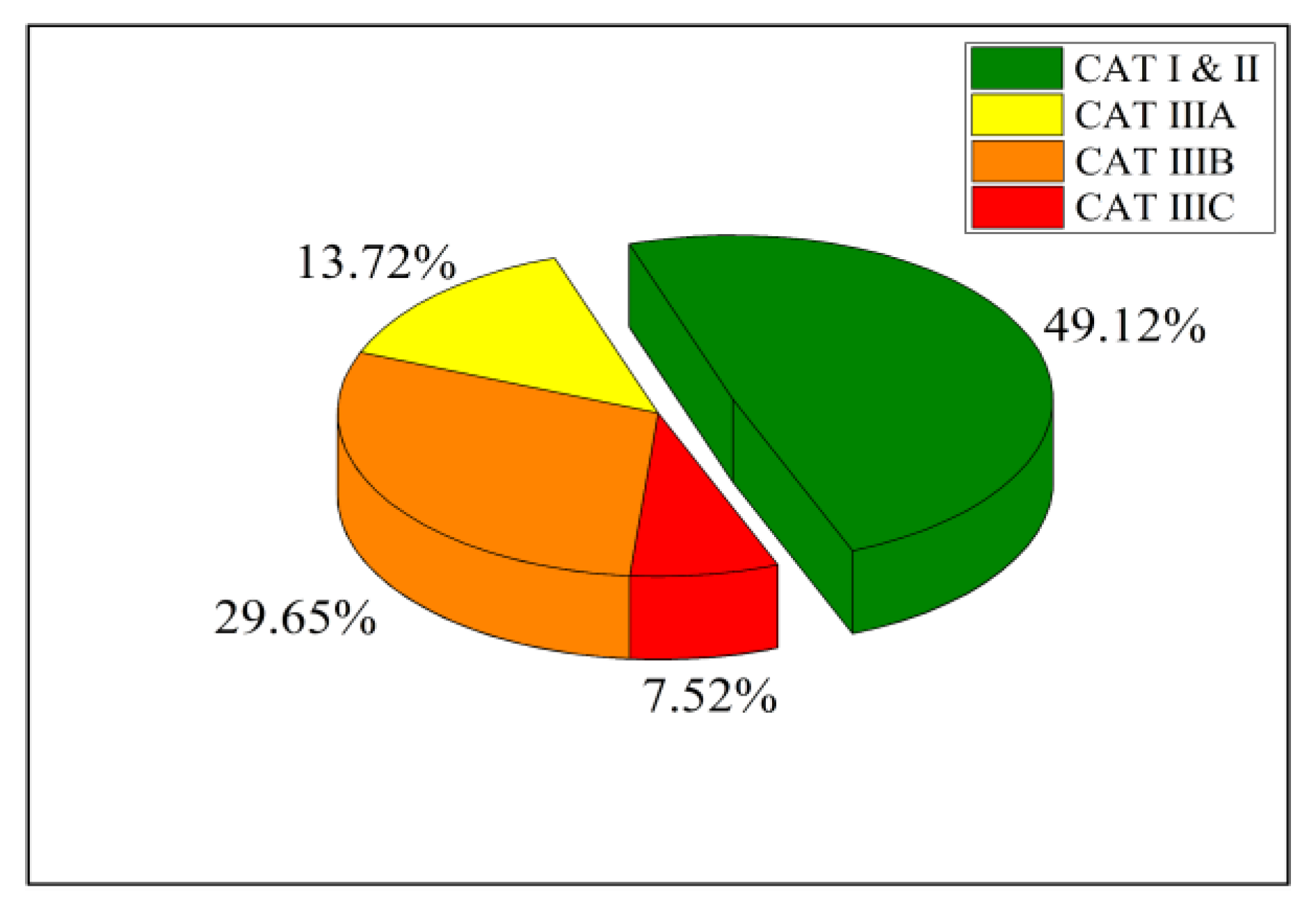
The World Meteorological Organization (WMO) defines fog as the reduction in visibility below 1000 m due to the suspension of tiny water droplets near the surface. The visibility in Delhi often drops below 1000 m during the winter without suspended water droplets in the air. The smaller suspended droplets formation was recorded at WiFEX observation site when the visibility fell below 500 m, which has been investigated using fog droplet measurements during the WiFEX campaigns. Therefore, the days when visibility (Vis) fell in the 500–1000 m range are generally referred to as hazy days, while those with Vis < 500 m are foggy days. As per the International Civil Aviation Organization (ICAO) guidelines, takeoff and landing of aircraft under visual flight rules (VFR) are not allowed when Vis < 500 m. Hence, we evaluated the forecasting skills for fog events when the visibility is below 500 m during the winter seasons of two years. Table 1 summarizes all fog events with the details about fog onset–lifting and total sustainment time in different visibility ranges. The category (CAT) of fog types based on different visibility ranges was established by the ICAO. Table 1 also represents the availability of ensemble-based forecasts at the IGI airport during the fog events of the study period. Figure 1 illustrates that the fog persists in the moderate fog category (includes both CAT I and CAT II; 550 m < Vis < 300 m) for almost 111 h (~49%), while for 115 h (~51%), fog was recorded in the dense fog category (CAT III). Typically, this optically thick and deep dense fog category [47] is the most challenging period for pilots and air traffic control (ATC) is to decide on take-off and landing of flights at runways.

Table 1.
Summary of observed fog events during WiFEX campaigns in 2020–2021 and 2021–2022 at the IGI airport, New Delhi, India.

Figure 1.
Fog classification is based on the four visibility ranges (CAT I and II, CAT IIIA, CAT IIIB, CAT IIIC) during the 2020–2021 and 2021–2022 winter months at IGI airport, New Delhi, India.
2.2. A Framework of EFS and Model Configurations
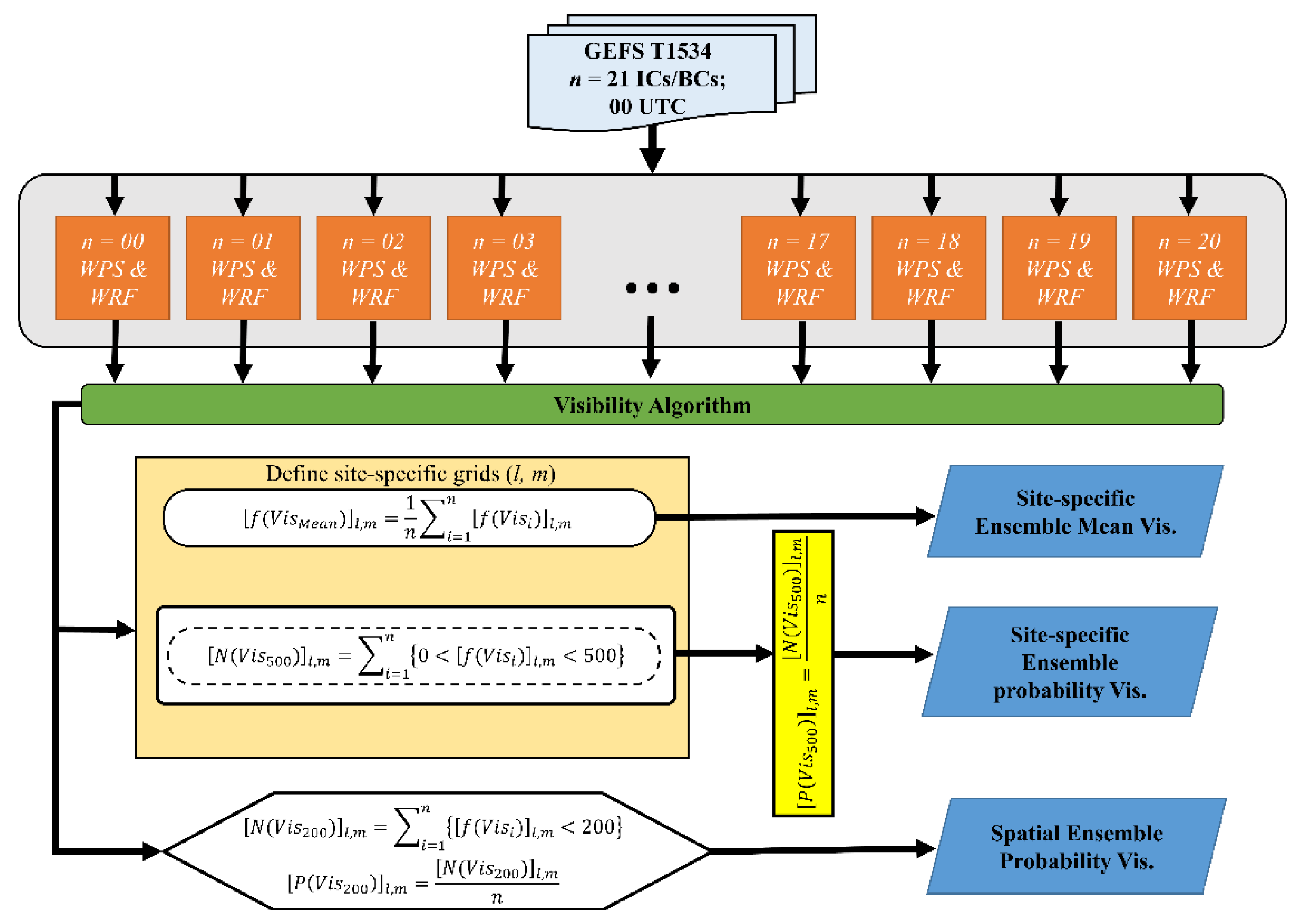
As part of the WiFEX 2020–2021 and 2021–2022 program, an earlier fog forecasting setup dedicated to the IGP region was reconfigured with the new EFS to provide daily 48-h forecasts during the winter months (December–January–February). This forecast is updated on WiFEX’s official site with bulletins (https://ews.tropmet.res.in/wifex/index.php). The EFS framework is a high-resolution 3D model-based ensemble fog prediction system. In the present study, 21 ICs/BCs at 0000 UTC from the Global Ensemble Forecast System (GEFS) were directly used to initialize the EFS. The EFS output is further post-processed by a visibility algorithm. The detailed working flowchart of the EFS is depicted in Figure 2. There was a need for an ensemble-based forecast system for region-specific probabilistic prediction of weather over India particularly for disastrous weather events, e.g., tropical cyclones, heavy rainfall events, etc. Considering the societal need into account, under the “Monsoon Mission” program, India’s MoES successfully implemented the Global Ensemble Forecast System (GEFS; semi-Lagrangian T574 L64 resolution) at IITM for seven days of weather prediction [42,48]. Furthermore, as per the need of forecasts at a block level (~12 km), the high-resolution ensemble prediction system (GEFS T1534) was implemented at IITM in June 2018 and subsequently handed over to the India Meteorological Department (IMD) for operational implementation. The GEFS suite comprises 21 ensemble members (1 control + 20 perturbed). n = 00 is the reference or control member (hereafter referred to as CNTL) and the other perturbed members (n = 01 to 20) are generated by the Ensemble Kalman Filter method with the forecast perturbation of the previous cycles four times a day at all 64 model vertical levels. To initialize the same number of 3D regional models, we directly utilized these 21 ICs/BCs. Advanced Research Weather Research and Forecasting (ARW) models, version 4.0, of 4 km horizontal resolution are used in the EFS [49]. Parallel arrangements of the 21 WRF models are specially designed to simulate the fog forecast. Technical specifications is common among all 21 WRF model setups, including domain configuration and model physics, except the ICs/BCs for their initialization. The specifications of the WRF model are discussed below.

Figure 2.
The schematic flowchart of the operational Ensemble Forecast System (EFS) for fog prediction by utilizing the perturbed initial conditions from the Global Ensemble Forecast System (GEFS) data at the Indian Institute of Tropical Meteorology (IITM), Pune, India.
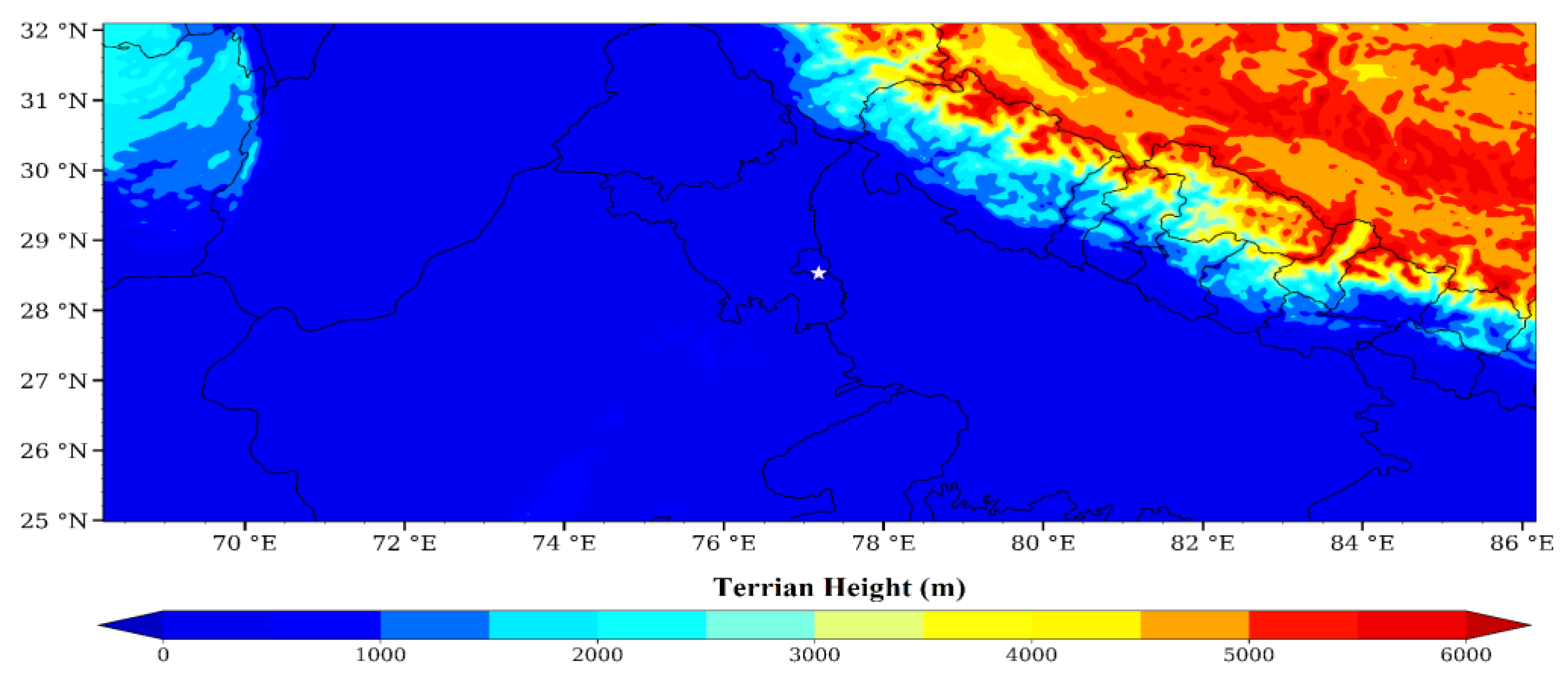
The single forecast domain, centered over Delhi (at 28.49° N, 77.10° E) and covering 1760 km in the east–west direction (440 grid points) and 800 km in the north–south direction (200 grid points), covers most of the fog-prone areas of North India, as shown in Figure 3. For a complete representation of the thermodynamic and surface processes within the planetary boundary layer (PBL), the vertical resolution of the WRF model is set at 60 sigma levels with dense vertical levels (19 levels) below 1000 m. In earlier studies, we evaluated multiple parameterization schemes (including PBL, microphysics, and land surface schemes) and model configurations (including domain size and horizontal/vertical resolutions) to determine the optimal model configuration for predicting dense fog events over North India [17,24,34]. Based on these sensitivity experiments, the model physical parameterization schemes in the present study include the local turbulent kinetic energy (TKE) closure Mellor–Yamada–Nakanishi–Niño Level 2.5 (MYNN2.5) PBL scheme, WSM6 microphysics, the CAM shortwave and longwave radiation scheme, and the Pleim–Xiu land surface model. The optimal configuration of EFS is briefly given in Table 2. From EFS, site-specific (area averaged of 8 km × 8 km horizontal resolution is selected for the site; l = latitude, m = longitude) visibility for each member is derived. These individual diagnosed visibility values (Vis < 500 m) are used to calculate the ensemble mean and the probability (P) of fog occurrence every hour over the IGI airport. In addition, each grid point of the domain is considered to calculate the spatial probability of dense fog (Vis = 200 m) over the IGP.

Figure 3.
A single domain (d01) of the ensemble forecasting system with horizontal resolution of 4 km cover the northern parts of India. The IGI airport in New Delhi, India, is represented with a star symbol.
Table 2.
Configuration of the WRF model used for the EFS in the study.
2.3. A Visibility-Based Diagnostic Method for Fog Prediction
The selection of an effective visibility algorithm is necessary to predict fog and evaluate the performance of the WRF model. The WRF model does not directly forecast horizontal visibility. Typically, the prognostic variables from WRF outputs, such as LWC, relative humidity, and temperature, are used for the visibility diagnostics [27]. Several studies showed that the LWC at the lowest model level was commonly used to represent fog [16,27,34]. Following the earlier Vis diagnostic approach suggested by [50,51,52,53], we developed a site-specific Vis parameterization as a function of fog index (FI is a product of LWC and fog droplet number concentration (Nd)) using microphysical measurements at the WiFEX observation site. In a highly polluted environment, Nd changes from a few hundred droplets to a few thousand droplets for nearly the same values of LWC [50,53,54]. By using the dataset of WiFEX 2017–2018, the fitting function is obtained. The fitting function correlates Vis and FI in a nearly linear manner [53] and the model predicted hourly LWC to calculate the FI. The fitting function indicates that the Vis is inversely related to LWC and Nd. Following the approach of [50], we also used maximum and minimum limiting values of Nd and LWC. The maximum limiting values for Nd and LWC used in the analysis are approximately 1000 cm−3 and 0.5 g m−3, respectively, while the minimum limiting Nd and LWC values are tens of cm−3 and 0.002 gm−3, respectively. The microphysical data beyond the abovementioned limit were excluded from the analysis. More details about the fitting function are documented elsewhere [53]. In the present study, since we used a single momentum microphysics scheme, we used a fixed value of Nd = 650 cm−3, based on the mean value from the microphysical observations. The fitting function obtained from observational datasets and simulated microphysical parameters (Nd and LWC) to estimate the Vis at the IGI airport is given in Equation (1). This equation is used for the two years of the operational forecast. The given visibility diagnostic approach recognizes the variability in droplet sizes and its role in reducing the visibility caused by fog. The hourly visibility values for each ensemble member were calculated at the IGI airport. Furthermore, the probability of fog occurrence based on visibility threshold values (Vis < 500 m) from 21 ensemble members was compared with the corresponding observed visibility values.
Vis = 1/[0.08 × (FI) + 0.37]
2.4. Forecast Skill Verification Methods
Dichotomous (binary) verification methods were used to verify a deterministic forecast against its corresponding observation for 39 fog events for 217 h at the IGI airport. Besides the CNTL forecasts, the probabilistic forecasts in EFS are also treated as deterministic forecasts with the given percentage threshold. Real ensemble NWP systems are naturally imperfect and they require statistical post-processing in order to generate calibrated probability forecasts for users. Generally, the ensemble mean or median (the 50% probability) forecast should have the most skill on average [37]. Since the prevailing number of ensemble members in this study is 21, the 50% probability threshold is applicable. Therefore, we used a 50% forecast to approximate the ensemble median forecast. Here, verification was only focused on the 24-hour forecasts. To verify both CNTL and EFS, a contingency table is used, which shows the frequency of “yes” and “no” forecasts and occurrences of fog events. The four combinations of forecasts (yes or no) and observations (yes or no), called the joint distribution, are listed below, where a, b, c, and d refer to event forecast to occur and did occur (hit), event forecast to occur but did not occur (false alarm), event forecast not to occur but did occur (miss), and event forecast not to occur and did not occur (correct negative), respectively. The following Equations (2)–(5) helped to represent the deterministic skill scores of forecasting systems.
Hit Rate (HR) = a/(a + c)
False Alarm Ratio (FAR) = b/(a + b)
Missing Rate (MR) = c/(a + c)
Critical Success Index (CSI) = a/(a + b+c)
However, we further evaluated the skill of EFS by a probabilistic method. For verifying ensemble probabilistic forecasts, Brier Score (BS), Brier Skill Score (BSS), Reliability diagram, Ensemble spread vs. ENS mean error, and a Relative Operating Characteristic (ROC) diagram were used. The BSS is derived from BS and BSr shown in Equations (6)–(8), respectively. The BS is the mean squared difference between the forecast probability and binary observation [55]. Here, i denotes the forecast number (out of the total number of forecasts), N is the total number of forecast–observation pairs for all forecasts, and Pi and Oi are the forecast probability and binary observation at the ith sample, respectively. The Pi ranges in value from 0 to 1, but the Oi is either 1 (yes event) or 0 (no event). As the BS is an error score, the lesser the BS, the better the forecast. Hence, a BS value of 0 indicates a perfect forecast. Similarly, the Brier Score for the reference forecast (BSr) is calculated (a single deterministic forecast), where FI ranges in value from 1 (yes) to 0 (no). The reliability diagram measures agreement between predicted probabilities and observed frequencies. The success of EFS is measured using ROC as it plots the hit rate against the false alarm rate with increasing probability thresholds. The area under the curve (ROC area) is helps to summarize the potential of forecast skills. An ROC curve along the diagonal indicates that the hit rate and false alarm rate are equal; hence, the forecast has no skill. A curve below the diagonal represents negative skill.
Brier Skill Score (BSS) = 1 − (BS/BSr)
3. Result and Discussions
3.1. The 19–20 January 2022 Fog Case
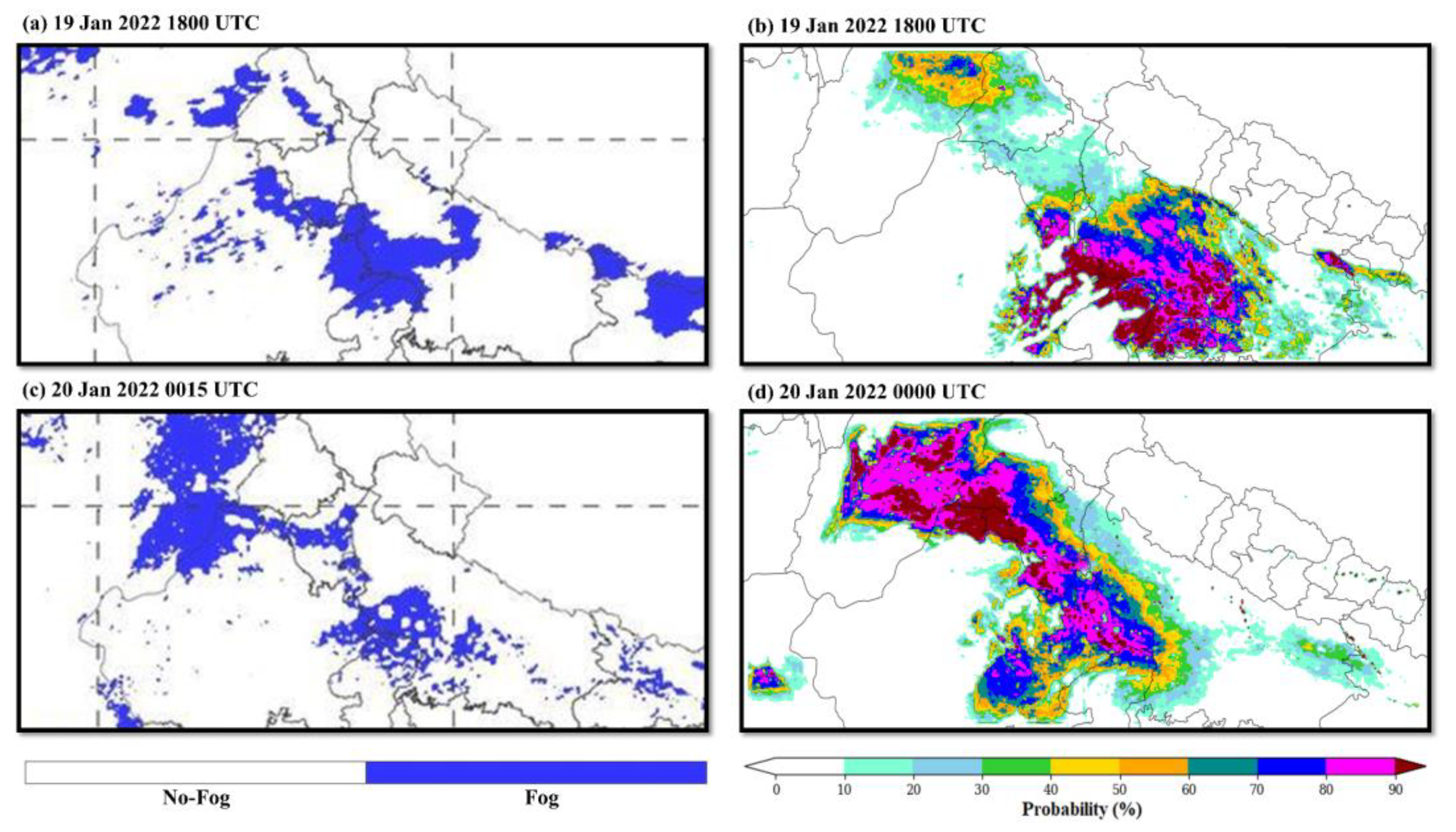
Figure 4 shows the resemblance between the observed INSAT-3DR satellite fog/low-cloud product with the ensemble probability forecast for a visibility threshold Vis < 200 m over the different parts of North India in the late evening and at midnight during the 19–20 January 2022 fog event. In the afternoon on 19 January, the northwest part of the IGP region was dominated by a high-pressure system that slowly progressed to the central part of India. As a result, nocturnal radiative cooling occurred over various parts of North India under stable atmosphere. From the satellite fog/cloud products shown in Figure 4a, it can be demonstrated that fog formed rapidly over the northwest part of Rajasthan, eastern parts of Uttar Pradesh, and southern parts of Delhi in the late evening on 19 January. However, sparse fog patches were seen over these locations and densely packed fog was seen over the northeast part of Punjab at midnight on 20 January. Within six hours before midnight fog occurrence, such a transformation of fog could be possible due to the windy conditions and the shifting high-pressure system (from synoptic charts and IMD report). Interestingly, the short-lived spatial state of this fog event and its unique characteristics are comprehensively captured in the ensemble probability forecast. At both late evening and midnight time stamps of EFS, more than 60% probability of fog occurrence shows over the foggy areas. This could suggests that the model played a significant role in simulating the fog event. EFS has shown its skill to simulate an optimal synoptic environment for fog formation on an operational level.

Figure 4.
(a,c) INSAT-3DR satellite fog/low-cloud product compared with (b,d) spatial ensemble probability forecast for visibility threshold Vis < 200 m over the study domain on 19–20 January 2022.
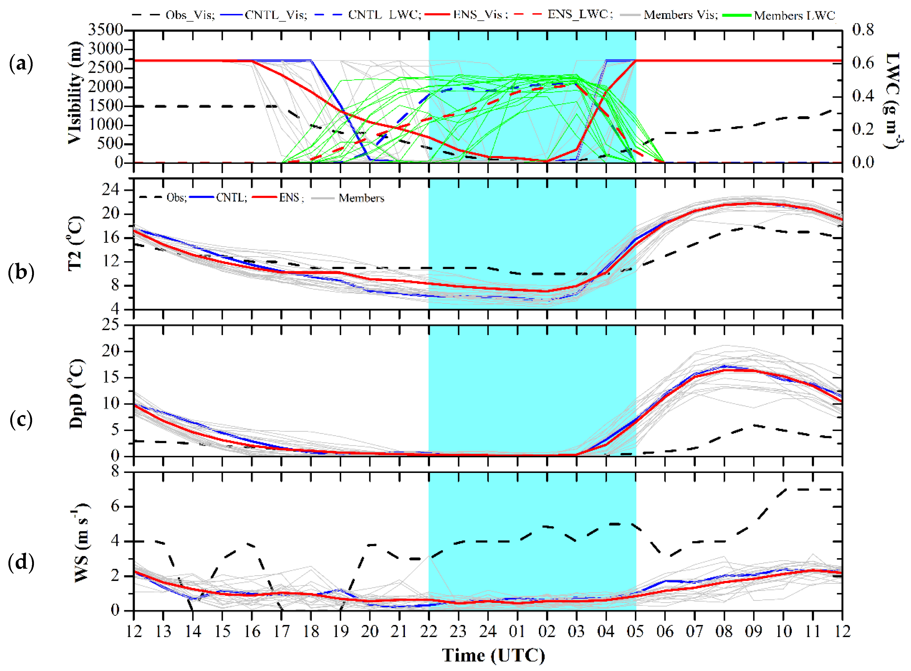
Figure 5a shows the temporal variation in the observed visibility versus simulated visibility and simulated LWC for the different ensemble members for the fog events that occurred over the IGI airport on 19–20 January 2022. Figure 5 illustrates that the diagnosed visibility is highly sensitive to the simulated values of LWC in each member. The fog (Vis < 500 m) initially developed at 2200 UTC on 19 January until the late morning of 0500 UTC on 20 January. In the CNTL forecast, the onset of fog based on diagnosed visibility is recorded at 2000 UTC on 19 January, which was noticed 2 h earlier (advancement) than the actual fog evolution. The ensemble mean (ENS) forecast represents accurate fog onset timing. To demonstrate meteorologically why ensemble-based fog forecasts work better than the CNTL forecast, the fog episode was examined with the observations shown in Figure 5b–d. Over the IGI airport, variations in predicted LWC among ensemble members were high, causing uncertainty in fog predictions (based on visibility) from member to member. Based on this, it is unlikely that a single member could capture the spread of the fog events, including its exact onset, sustainment, and burn-off period. In fact, a single fog case might be predicted by a few members of the ensemble system and missed by other members. For instance, in the present study, ensemble members no. 06 and 08 (gray color lines which were not highlighted) captured all meteorological fields better than other ensemble members; however, this will not always happen during other fog events. Similar success or failure in accurate meteorology prediction during fog events could also be conjectured in the CNTL forecast. In contrast, the ensemble mean generally provides a better forecast than any of the individual ensemble members, regardless of the width or shape of the distribution of members around the mean. In the present case study, ENS captured the characteristics of the ideal meteorological variables to accurately represent the LWC and fog lifecycle rather than the CNTL forecast. The bias in the 2 m temperature of ENS is less than 3 K (slight cold bias), especially during the fog period. The simulated under-predicted wind speed in CNTL and ENS roughly captured the trend of airflow after onset of the fog. The bias in DpD of ENS is zero and exactly matched at the time of fog onset. Thus, the onset of fog is accurately represented in the ENS compared to the CNTL. However, ENS and CNTL recorded fog-lifted time at around 0300 UTC, which is 2 h earlier than the actual lifting of the fog. All perturbed members including CNTL simulations burned off the fog before 0400 UTC on 20 January 2022 by sudden increases in T2 and DpD values. This could indicate the lacuna of radiation parameterization and the absence of chemistry composition in the present model, which can burn off the fog at surface and lifted it quickly after the sunrise irrespective of how accurate ICs/BCs are. Furthermore, we extended our study by investigating the probability forecast skill of EFS. Probability forecasts are most effective when users choose a probability threshold that provides the right balance between alerts and false alarms.

Figure 5.
Temporal variation in observed versus simulated (a) visibility (m) and LWC (g m−3), (b) temperature at 2 m (T2, °C), (c) dew point depression at 2 m (DpD, °C), and (d) wind speed at 10 m (WS, m s−1) at IGI airport, New Delhi, India, on 19–20 January 2022.
3.2. Skill Verification of Single Deterministic Forecast Versus Ensemble-Based Forecasts
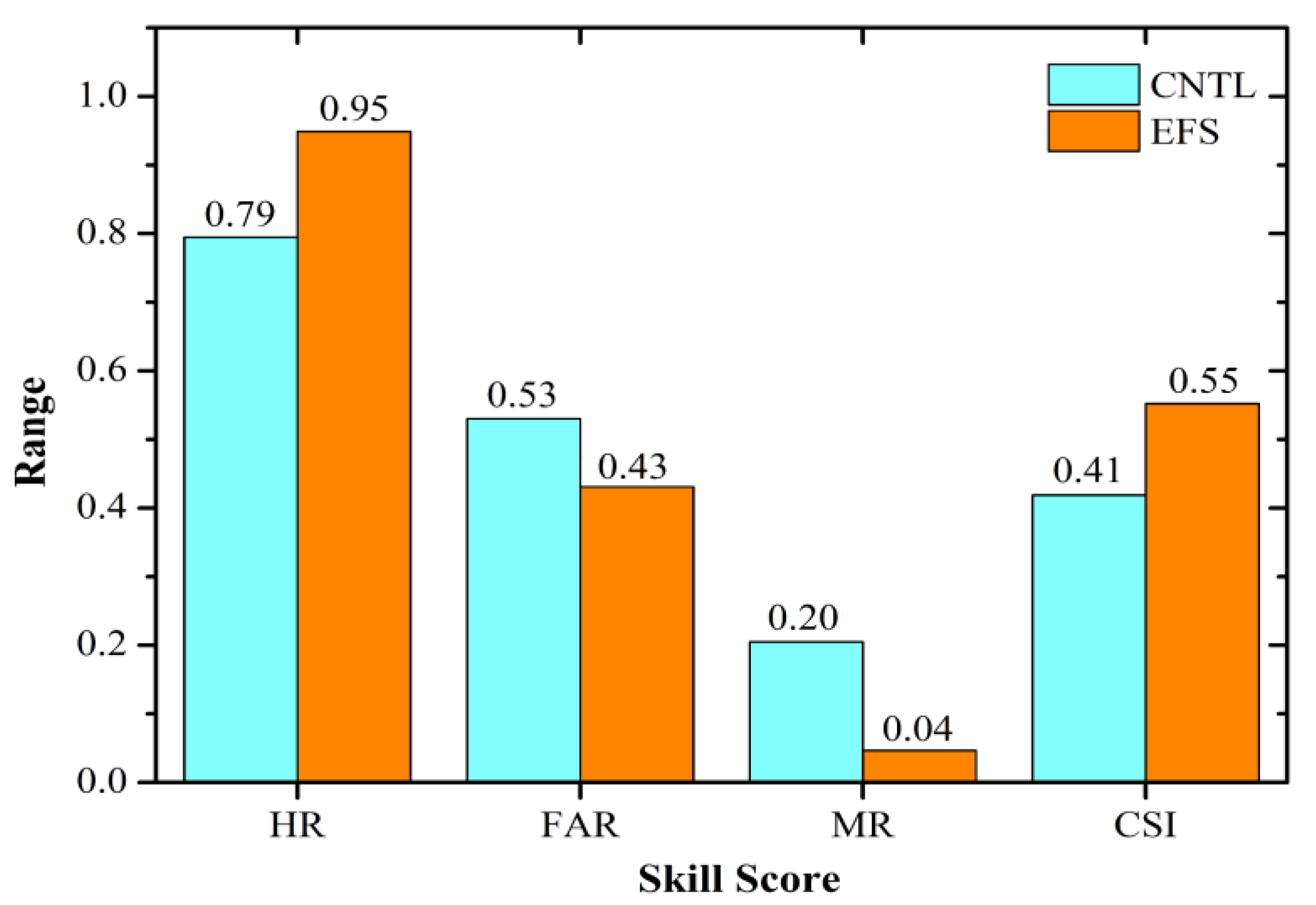
During the 2020–2021 and 2021–2022 winter periods, 41 fog events (Vis < 500 m) were recorded at the IGI airport. Due to some technical issues, forecasts are not generated on 7–8 December 2020 or 10–11 January 2021; therefore, these events were not considered during the skill evaluation. Figure 6 shows the deterministic skill scores measured (HR, FAR, MR, CSI) for control members (n = 00; CNTL) and 21 ensemble members (50% probability threshold) for Vis < 500 m at the IGI airport, New Delhi, India. We found that the skill of the EFS is better than the CNTL setup. The HR for EFS is much higher (0.95) than for the CNTL forecasts (0.79). The HR indicates the percentage of correctly predicted fog and non-fog events, the most direct measure of accuracy for the binary forecasts. In addition, the MR in EFS is lower (0.04) than the CNTL (0.21). Although the value of FAR is high in both EFS and CNTL, the ensemble method has less FAR (0.43) than the CNTL (0.53). By combining HR, FAR, and MR, we can estimate the CSI, which measures the fraction of observed and/or forecast events, which are correctly predicted. The CSI for EFS is approximately 0.55, while for CNTL, the CSI is 0.42. The HR and CSI for EFS are relatively promising, with values of 0.94 and 0.55, respectively. These values are higher than the median value of 0.5, which indicates that the EFS has reasonable accuracy in predicting fog events.

Figure 6.
Forecasting skill scores (Hit Rate, False Alarm Ratio, Missing Rate, and Critical Success Index) of control (n = 00; CNTL) and 21-member ensemble forecast system during the winter season of 2020–2021 and 2021–2022 at IGI airport, New Delhi, India.
The ensemble-based forecasts show a BS of 0.13, which implies less error between the forecast probabilities and observed occurrence or non-occurrence of fog events. Moreover, the BS is typically converted into a BSS by normalizing it against a reference forecast. Here, a BSS of 1.0 indicates a perfect forecast, while a BSS of 0.0 indicates the skill of the reference forecast. Interestingly, the higher value of BSS (0.67) in the present study shows better accuracy of the probabilistic forecast relative to the reference forecast, and EFS with a 50% probability threshold could correctly predict 37 (out of 39) fog events, while the reference deterministic forecasts could predict 31 (out of 39) fog events. The components of the Brier Score decomposition can be used to assess the reliability (Brel) and resolution (Bres) of the forecast attributes, as well as the inherent uncertainty of the underlying processes that are relevant for the interpretation of the sources of errors in the forecasts [56], which is useful for exploring the dependence of probability forecasts on ensemble characteristics. The Brel value measures the difference between the forecast and the mean observation associated with that forecast value over all the forecasts. Regarding the Bres measure, if the forecasts sort the observations into sub-samples having substantially different relative frequencies than the overall sample climatology, the resolution term will be large. This is a desirable situation, since the resolution term is subtracted. The resolution term is large if there is enough resolution to produce very high and very low probability forecasts. In the present study, estimated values of Brel and Bres are 0.10 and 0.06, respectively.
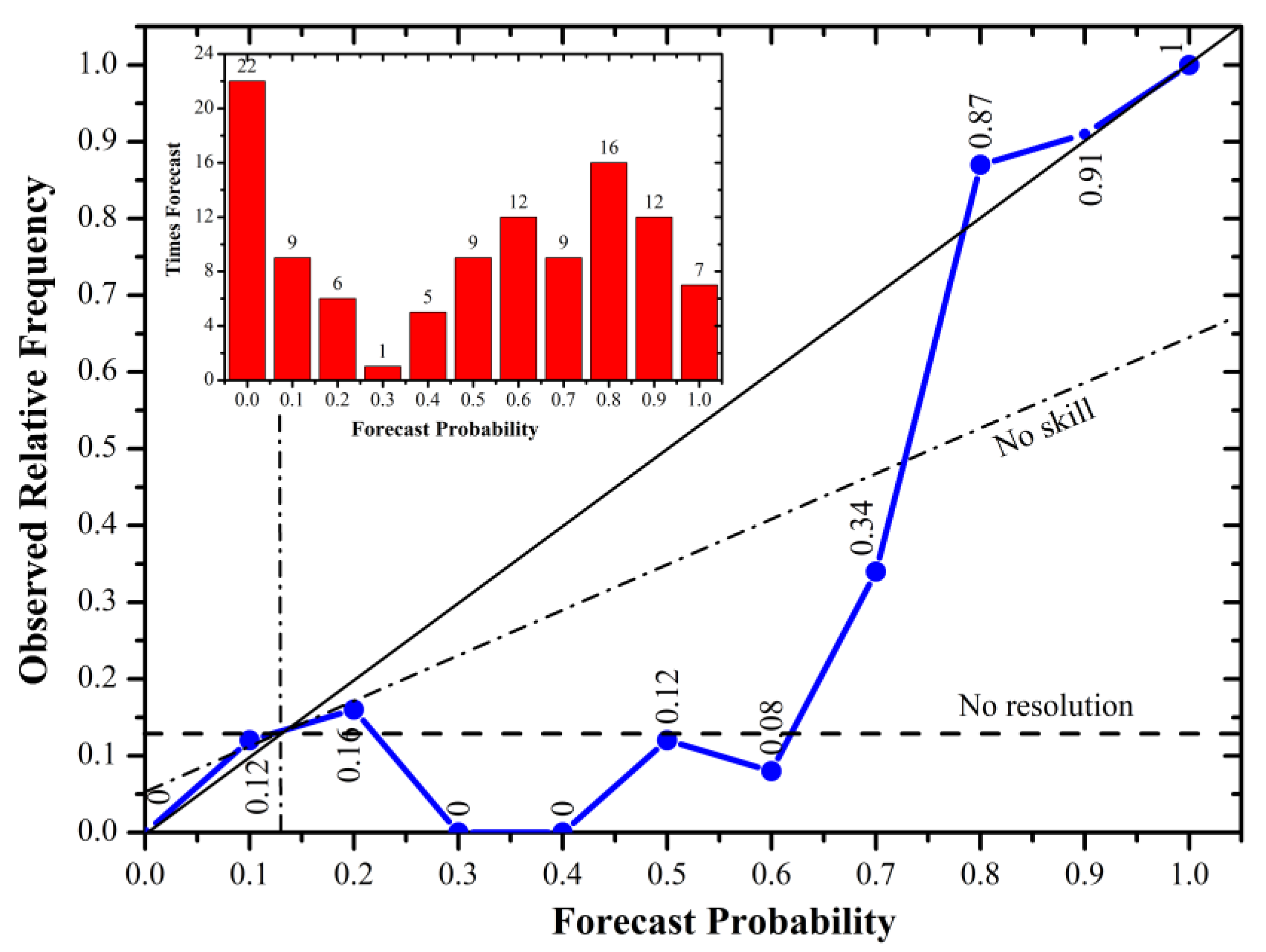
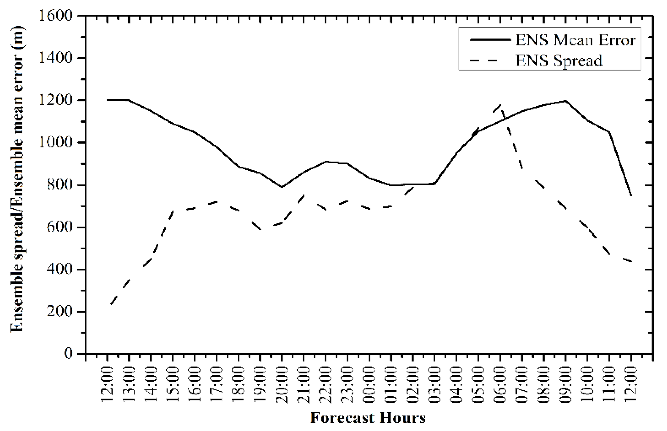
In addition, the reliability diagram measures the accuracy with which a discrete event is forecast by a probabilistic forecasting system. Figure 7 depicts that the reliability diagram curve for mid-range probability values is below the no skill line, while for the higher forecast probability values (P > 70%), it is above the no resolution line. In case of medium-range probability values (20% < P < 60%), it is indicating that the probability is under-sampled. Despite the position of the curve, it is not flat and rises with increasing forecast probability categories. This indicates the ability of the forecast to be more skillful than the climatology. As the curve is below the diagonal, we can deduce that the forecast is overconfident, which implies that with increasing forecast probability categories, it produces more forecasts than the observed occurrences. However, from the sharpness diagram, the ensemble spread too large where most observations fall near the higher forecast probability values. Figure 8 shows the ensemble mean error (ENS error) and the spread variation with forecast lead hours (24 h forecast) for EFS. It is observed that ENS error and spread behave in opposite ways before and after fog hours, which is attributed to limitation of the visibility algorithm. Here, a spread smaller than the ENS error indicates that the forecast is overconfident and thus, the ensemble system is under-dispersive.

Figure 7.
Reliability diagram for ensemble probability forecast for all fog cases.

Figure 8.
Ensemble spread and ENS mean error.
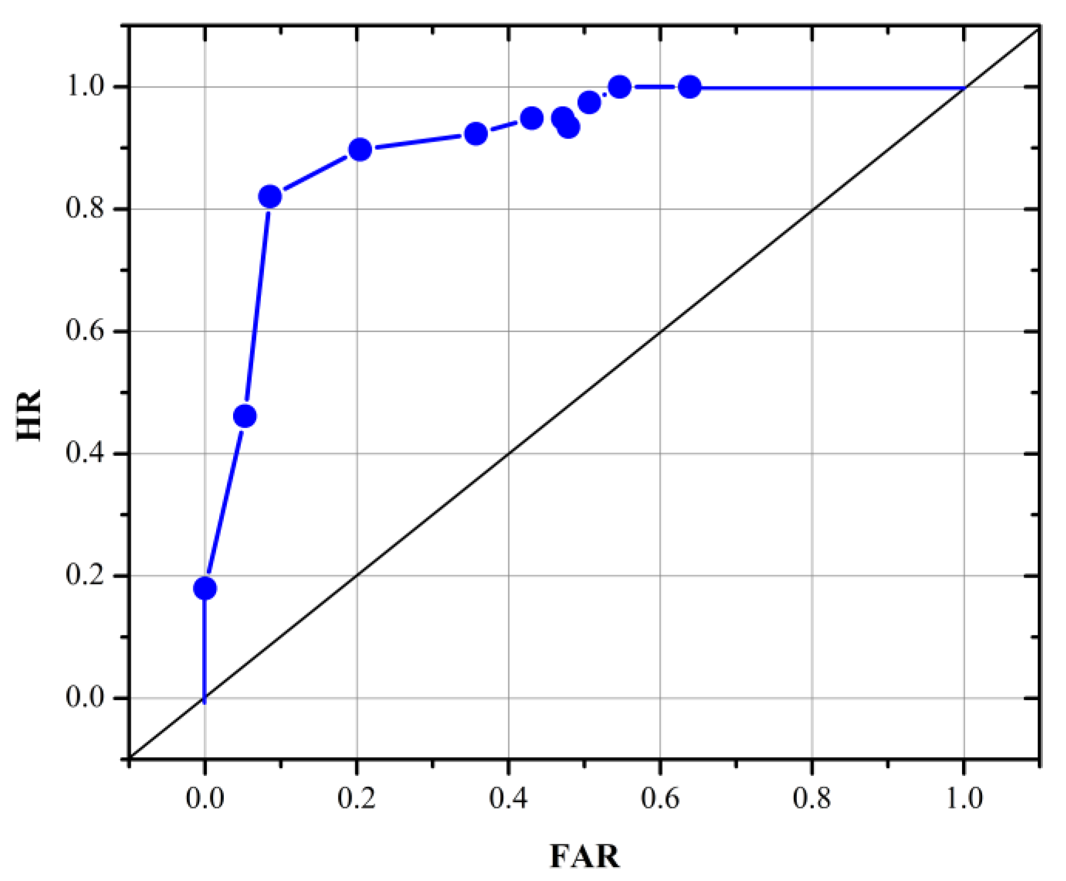
Figure 9 shows the ROC curve from the comparison of 2 years of ensemble-based model forecast and observation pairs. Since ROC is independent of forecast bias, it shows the potential skill of the forecast. The ROC curve is constructed by setting the probability threshold in 10% increments to calculate the hit rates and false alarm rates. Over the 2 years of winter period verification, the EFS performs well and has an ROC score (fractional area under the curve) of 0.88, thus quantifying the skillful forecast. The near-perfect curve shows high resolution in the forecast, indicating the ability of the forecast to discriminate among the different forecast probabilities. At each 10% probability increment, the EFS hit rate is relatively higher than the false alarm rate, with a maximum difference between the HR and FAR of 0.7 at a probability of 90%. Thus, the EFS accurately predicts the fog events over the IGI airport. This shows that a probability between 0–20% and 80–100% is the threshold at which the EFS performs the best at discriminating between regions of no fog and fog compared to the observed fog events.

Figure 9.
Relative Operating Characteristic (ROC) diagram of probabilistic forecasts based on the 21-member ensemble forecast system for IGI airport, New Delhi, India.
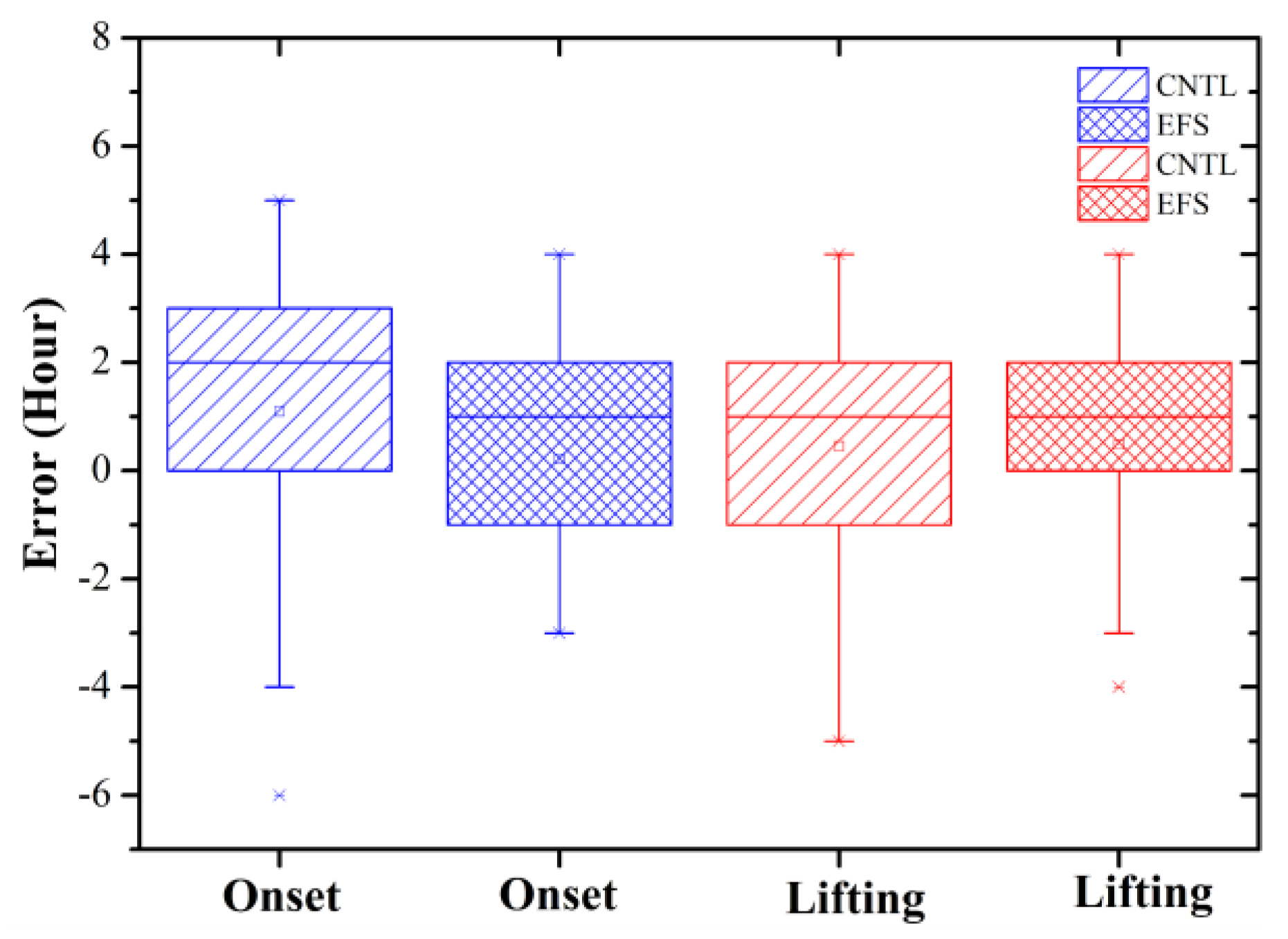
Figure 10 shows the box-and-whisker plot of fog onset and fog lifting error (between predicted and observed) for the fog events observed at the IGI airport. We found that the EFS predicted the onset and lifting of fog relatively well compared to CNTL. For onset, the mean error was close to 1 h (2 h) in EFS (CNTL), while for fog lifting, it was close to 1 h in both forecasting setups. In addition, the box and whisker plot is utilized to visualize dataset skewness (this conveys whether deviations from the median are more likely to be positive or negative). In CNTL forecasts, the onset and lifting error median is shifted toward the upper portion of the box, with a wider range of datasets in the lower quartile than the upper quartile, indicating negative skewness. Similar negative skewness can be noticed in the EFS onset error but with a large interquartile range compared to the whiskers (showing the clustering of the dataset near the 25th and 75th percentile). In contrast, the skewness is zero in the EFS lifting error case. The onset and lifting of fog strongly depend on the balance among the land surface processes, radiative cooling, moisture subsidence, and turbulence during the fog lifecycle. From the box-and-whisker plot, it is clear that these kinds of balancing could be better captured in the EFS. Therefore, the EFS has reduced the errors in the fog onset and dissipation relative to the CNTL. Overall, the above results show that the ensemble-based forecasts (50% probability threshold) with a visibility threshold Vis < 500 m have better efficiency than deterministic forecasts.

Figure 10.
Box-and-whisker plot of onset and lifting error (hours) in control (CNTL) and ensemble-based forecast (EFS) for all observed fog events (Vis < 500 m) at IGI airport, New Delhi, India.
The high-resolution GEFS is a weather model that generates 21 ensemble members to address underlying uncertainties in the input data such as limited coverage, biases in instruments or observing systems, and the limitations of the model itself. We directly used these ICs/BCs in a model of the EFS. GEFS quantifies these uncertainties by generating multiple ensemble members, which in turn produce a range of potential outcomes based on differences or perturbations applied to the data after they have been incorporated into the model. Since each member compensates for a different set of uncertainties, the EFS could be advantageous by providing the approach for incorporating both initial conditions and model uncertainty into the fog forecast process while automatically accounting for flow dependence. However, the present EFS has several limitations. For instance, (a) the present system is associated with a high computational cost and often involve statistical post-processing steps to inexpensively improve its raw prediction qualities. (b) Even after incorporating the multiple ICs/BCs with optimized physics options, there is still an error in mean fog onset and lifting time. This could be attributed to the lacuna in the physics options of the model. (c) FAR in the present EFS is relatively high. One of the reasons could be the high moisture bias in more than 50% of ensemble members’ simulations. This high moisture bias directly caused an overestimation of the LWC value in simulations, leading to reduced visibility values compared to the observations. Through land surface data assimilation, it could be possible to reduce such micro-meteorological biases directly [24]. (d) The present visibility algorithm does not include the chemistry information. This could be one of the reasons for increasing the FAR. The chemical composition and hygroscopicity of aerosols determine the activation properties of aerosols in a polluted environment. Hygroscopically grown aerosol particles in sub-saturated conditions (hydrated aerosols) and fog droplets play significant roles in visibility fluctuation by scattering and absorbing visible radiation in heavily polluted conditions [27]. We did not extend our explanation to different fog categories due to the absence of such chemistry information in visibility parameterization. In the future, we will introduce the chemistry factors in visibility parameterization and report the visibility forecast for different fog categories at the IGI airport. This may further improve the forecast skill and decision quality of EFS for fog forecasting.
4. Summary and Conclusions
The present study proposed a new operational Ensemble Forecast System (EFS) to predict fog over the Indo-Gangetic Plain (IGP) region based on the visibility diagnostic algorithm. The EFS framework is based on the Weather Research and Forecasting (WRF) model with a single high-resolution (4 km horizontal resolution) fog forecasting domain, initialized parallelly by 21 initial/boundary conditions (ICs/BCs), available from the Global Ensemble Forecast System (GEFS) dataset (1 control + 20 perturbed). The EFS product facilitated the probability of fog occurrence (relative frequency) over different parts of North India and at one of the world’s busiest airports, the Indira Gandhi International (IGI) airport, New Delhi, India. The probability of fog occurrence has been calculated based on all individual members. In order to gain confidence in ensemble-based forecasts compared to the single deterministic forecasts (CNTL), we verified the skill of these fog forecasting systems for a visibility threshold Vis < 500 m during the 2020–2021 and 2021–2022 winter seasons (December–January) at the IGI airport. In this, EFS skill of can be evaluated probabilistically and deterministically. The probability threshold of 50% was used to consider a probabilistic fog forecast as a deterministic forecast. Verification was only focused on the 24-h forecasts. Before forecast skill verification, a successfully forecasted dense fog event was investigated in detail. The results showed that the EFS spatial product for a visibility threshold Vis < 200 m reasonably predicts the probability of the fog occurring over the different parts of North India in the late evening and at midnight during the 19–20 January 2022 fog event. In addition, the 21-member ensemble mean (ENS) product accurately captured the fog onset time with minimum bias in ideal fog meteorology compared to the CNTL forecast. Furthermore, the probabilistic skill also shows the better performance of EFS. The skill of EFS is reliable, with approximately 95% successful prediction of the fog events [Hit Rate (HR) = 0.95; False Alarm Ratio (FAR) = 0.43; Missing Rate (MR) = 0.04; Critical Success Index (CSI) = 0.55] at the IGI airport. The ensemble-based forecasts show a Brier Sore (BS) is 0.13, indicating less error between the forecast probabilities and observed occurrence or non-occurrence of fog events. From the reliability diagram, we noticed that the forecast is overconfident. Moreover, the higher value of the Brier Skill Score (BSS = 0.67) and the area under the Relative Operating Characteristic (ROC = 0.88) curve show better accuracy and the potential skill of the probabilistic forecast. This demonstrates the advantage of the EFS over the single deterministic forecast. Fog onset and lifting error analysis revealed that the EFS reduced the errors in the fog onset and dissipation relative to the CNTL. Overall, this could suggest that the EFS used in the present study for the real-time fog forecast achieved physically realistic conditions compared to a single deterministic forecast and that after modifying the visibility algorithm and improvement in the initial soil fields, it could serve as a decision support system for fog forecasting at various airports to mitigate fog-related losses.
Author Contributions
Conceptualization, A.N.P., S.D.G. and G.G.; Methodology, A.N.P., S.D.G., N.G.D., G.G. and M.B.; Experiment and Analysis, A.N.P., S.D.G., N.G.D., P.L., S.W., G.G., M.B. and R.K.J.; Writing, A.N.P., S.D.G., N.G.D., G.G. and M.B.; Supervision, S.D.G. and G.G. All authors have read and agreed to the published version of the manuscript.
Funding
This research received no external funding.
Institutional Review Board Statement
Not applicable.
Informed Consent Statement
Not applicable.
Data Availability Statement
The statement should be excluded. All data are shown in the tables of the text.
Acknowledgments
Support and encouragement by the Director, IITM, Head, NCMRWF, DG, IMD and Secretary, MoES, in implementing the EFS system is gratefully acknowledged. MoES High Power Computing (HPC) facilities “Pratyush” and “Aditya” located at IITM, Pune, “MIHIR” situated in Noida, and their support team are highly appreciated and acknowledged. The authors express their sincere gratitude to Narendra Nigam, Arun S.H., and all officials met at the IGI airport, New Delhi, for their support and data provision during the study. We express sincere thanks to V. S. Prasad, P. Mukhopadhyay, R. Phani Murali Krishna, Prakash Pithani, Medha Deshpande, and Snehlata Tirkey for their support. We would also like to thank Shubhangi Ingle for WiFEX website development and technical support.
Conflicts of Interest
The authors declare no conflict of interest.
References
- Singh, J.; Kant, S. Radiation Fog over North India during Winter from 1989–2004. Mausam 2006, 57, 271–290. [Google Scholar] [CrossRef]
- Jenamani, R.K. Micro-Climatic Study and Trend Analysis of Fog Characteristics at IGI Airport New Delhi Using Hourly Data (1981–2005). Mausam 2012, 63, 203–218. [Google Scholar] [CrossRef]
- Kutty, S.G.; Dimri, A.P.; Gultepe, I. Climatic Trends in Fog Occurrence over the Indo-Gangetic Plains. Int. J. Climatol. 2019, 40, 2048–2061. [Google Scholar] [CrossRef]
- Ghude, S.D.; Bhat, G.S.; Prabhakaran, T.; Jenamani, R.K.; Chate, D.M.; Safai, P.D.; Karipot, A.K.; Konwar, M.; Pithani, P.; Sinha, V.; et al. Winter Fog Experiment over the Indo-Gangetic Plains of India. Curr. Sci. 2017, 112, 767–784. [Google Scholar] [CrossRef]
- Dhangar, N.G.; Parde, A.N.; Ahmed, R.; Prasad, D.S.V.V.; Lal, D.M. Fog Nowcasting over the IGI Airport, New Delhi, India Using Decision Tree. Mausam 2022, 4, 785–794. [Google Scholar]
- Dietz, S.J.; Kneringer, P.; Mayr, G.J.; Zeileis, A. Forecasting Low-Visibility Procedure States with Tree-Based Statistical Methods. Pure Appl. Geophys. 2019, 176, 2631–2644. [Google Scholar] [CrossRef]
- Lindner, B.L.; Mohlin, P.J.; Caulder, A.C.; Neuhauser, A. Development and Testing of a Decision Tree for the Forecasting of Sea Fog Along the Georgia and South Carolina Coast. J. Oper. Meteorol. 2018, 6, 47–58. [Google Scholar] [CrossRef]
- Marzban, C.; Leyton, S.; Colman, B. Ceiling and Visibility Forecasts via Neural Networks. Weather Forecast. 2007, 22, 466–479. [Google Scholar] [CrossRef]
- Colabone, R.d.O.; Ferrari, A.L.; Vecchia, F.A.d.S.; Tech, A.R.B. Application of Artificial Neural Networks for Fog Forecast. J. Aerosp. Technol. Manag. 2015, 7, 240–246. [Google Scholar] [CrossRef]
- Ribaud, J.F.; Haeffelin, M.; Dupont, J.C.; Drouin, M.A.; Toledo, F.; Kotthaus, S. PARAFOG v2.0: A near-Real-Time Decision Tool to Support Nowcasting Fog Formation Events at Local Scales. Atmos. Meas. Tech. 2021, 14, 7893–7907. [Google Scholar] [CrossRef]
- Mitra, A.K.; Nath, S.; Sharma, A.K. Fog Forecasting Using Rule-Based Fuzzy Inference System. J. Indian Soc. Remote Sens. 2008, 36, 243–253. [Google Scholar] [CrossRef]
- Bari, D. Visibility Prediction Based on Kilometric NWP Model Outputs Using Machine-Learning Regression. In Proceedings of the IEEE 14th International Conference on eScience, e-Science, Amsterdam, The Netherlands, 29 October–1 November 2018. [Google Scholar]
- Bari, D.; Ouagabi, A. Machine-Learning Regression Applied to Diagnose Horizontal Visibility from Mesoscale NWP Model Forecasts. SN Appl. Sci. 2020, 2, 556. [Google Scholar] [CrossRef]
- Dewi, R.; Prawito; Harsa, H. Fog Prediction Using Artificial Intelligence: A Case Study in Wamena Airport. J. Phys. Conf. Ser. 2020, 1528, 012021. [Google Scholar] [CrossRef]
- Castillo-Botón, C.; Casillas-Pérez, D.; Casanova-Mateo, C.; Ghimire, S.; Cerro-Prada, E.; Gutierrez, P.A.; Deo, R.C.; Salcedo-Sanz, S. Machine Learning Regression and Classification Methods for Fog Events Prediction. Atmos. Res. 2022, 272, 106157. [Google Scholar] [CrossRef]
- Pithani, P.; Ghude, S.D.; Chennu, V.N.; Kulkarni, R.G.; Steeneveld, G.J.; Sharma, A.; Prabhakaran, T.; Chate, D.M.; Gultepe, I.; Jenamani, R.K.; et al. WRF Model Prediction of a Dense Fog Event Occurred During the Winter Fog Experiment (WIFEX). Pure Appl. Geophys. 2019, 176, 1827–1846. [Google Scholar] [CrossRef]
- Yadav, P.; Parde, A.N.; Dhangar, N.G.; Govardhan, G.; Lal, D.M.; Wagh, S.; Prasad, D.S.V.V.D.; Ahmed, R.; Ghude, S.D. Understanding Genesis of a Dense Fog Event over Delhi Using Observations and High-Resolution Model Experiments. Model. Earth Syst. Environ. 2022, 136, 1–12. [Google Scholar] [CrossRef]
- Steeneveld, G.J.; Ronda, R.J.; Holtslag, A.A.M. The Challenge of Forecasting the Onset and Development of Radiation Fog Using Mesoscale Atmospheric Models. Bound. Layer Meteorol. 2014, 154, 265–289. [Google Scholar] [CrossRef]
- Pithani, P.; Ghude, S.D.; Prabhakaran, T.; Karipot, A.; Hazra, A.; Kulkarni, R.; Chowdhuri, S.; Resmi, E.A.; Konwar, M.; Murugavel, P.; et al. WRF Model Sensitivity to Choice of PBL and Microphysics Parameterization for an Advection Fog Event at Barkachha, Rural Site in the Indo-Gangetic Basin, India. Theor. Appl. Climatol. 2019, 136, 1099–1113. [Google Scholar] [CrossRef]
- Kutty, S.G.; Dimri, A.P.; Gultepe, I. Physical Processes Affecting Radiation Fog Based on WRF Simulations and Validation. Pure Appl. Geophys. 2021, 178, 4265–4288. [Google Scholar] [CrossRef]
- Steeneveld, G.J.; de Bode, M. Unravelling the Relative Roles of Physical Processes in Modelling the Life Cycle of a Warm Radiation Fog. Q. J. R. Meteorol. Soc. 2018, 144, 1539–1554. [Google Scholar] [CrossRef]
- Pagowski, M.; Gultepe, I.; King, P. Analysis and Modeling of an Extremely Dense Fog Event in Southern Ontario. J. Appl. Meteorol. 2004, 43, 3–16. [Google Scholar] [CrossRef]
- Spirig, R.; Vogt, R.; Larsen, J.A.; Feigenwinter, C.; Wicki, A.; Franceschi, J.; Parlow, E.; Adler, B.; Kalthoff, N.; Cermak, J.; et al. Probing the Fog Life Cycles in the Namib Desert. Bull. Am. Meteorol. Soc. 2019, 100, 2491–2507. [Google Scholar] [CrossRef]
- Parde, A.N.; Ghude, S.D.; Sharma, A.; Dhangar, N.G.; Govardhan, G.; Wagh, S.; Jenamani, R.K.; Pithani, P.; Chen, F.; Rajeevan, M.; et al. Improving Simulation of the Fog Life Cycle with High-Resolution Land Data Assimilation: A Case Study from WiFEX. Atmos. Res. 2022, 278, 106331. [Google Scholar] [CrossRef]
- Price, J.D.; Lane, S.; Boutle, I.A.; Smith, D.K.E.; Bergot, T.; Lac, C.; Duconge, L.; McGregor, J.; Kerr-Munslow, A.; Pickering, M.; et al. LANFEX : A Field and Modeling Study to Improve Our Understanding and Forecasting of Radiation Fog. Bull. Am. Meteorol. Soc. 2018, 99, 2061–2077. [Google Scholar] [CrossRef]
- Haeffelin, M.; Bergot, T.; Elias, T.; Tardif, R.; Carrer, D.; Chazette, P.; Colomb, M.; Drobinski, P.; Dupont, E.; Dupont, J.C.; et al. PARISFOG: Shedding New Light on Fog Physical Processes. Bull. Am. Meteorol. Soc. 2010, 91, 767–783. [Google Scholar] [CrossRef]
- Gultepe, I.; Pearson, G.; Milbrandt, J.A.; Hansen, B.; Platnick, S.; Taylor, P.; Gordon, M.; Oakley, J.P.; Cober, S.G. The Fog Remote Sensing and Modeling Field Project. Bull. Am. Meteorol. Soc. 2009, 90, 341–360. [Google Scholar] [CrossRef]
- Fernando, H.J.S.; Gultepe, I.; Dorman, C.; Pardyjak, E.; Wang, Q.; Hoch, S.; Richter, D.; Creegan, E.; Gaberšek, S.; Bullock, T.; et al. C-FOG: Life of Coastal Fog. Bull. Am. Meteorol. Soc. 2021, 102, E244–E272. [Google Scholar] [CrossRef]
- Wagh, S.; Krishnamurthy, R.; Wainwright, C.; Wang, S.; Dorman, C.E.; Fernando, H.J.S.; Gultepe, I. Study of Stratus-Lowering Marine-Fog Events Observed During C-FOG. Bound. Layer Meteorol. 2021, 181, 317–344. [Google Scholar] [CrossRef]
- Jayakumar, A.; Rajagopal, E.N.; Boutle, I.A.; George, J.P.; Mohandas, S.; Webster, S.; Aditi, S. An Operational Fog Prediction System for Delhi Using the 330 m Unified Model. Atmos. Sci. Lett. 2018, 19, e796. [Google Scholar] [CrossRef]
- Bott, A.; Trautmann, T. PAFOG—A New Efficient Forecast Model of Radiation Fog and Low-Level Stratiform Clouds. Atmos. Res. 2002, 64, 191–203. [Google Scholar] [CrossRef]
- Bergot, T.; Koracin, D. Observation, Simulation and Predictability of Fog: Review and Perspectives. Atmosphere 2021, 12, 235. [Google Scholar] [CrossRef]
- Bergot, T.; Carrer, D.; Noilhan, J.; Bougeault, P. Improved Site-Specific Numerical Prediction of Fog and Low Clouds: A Feasibility Study. Weather Forecast. 2005, 20, 627–646. [Google Scholar] [CrossRef]
- Pithani, P.; Ghude, S.D.; Jenamani, R.K.; Biswas, M.; Naidu, C.V.; Debnath, S.; Kulkarni, R.; Dhangar, N.G.; Jena, C.; Hazra, A.; et al. Real-Time Forecast Of Dense Fog Events Over Delhi: The Performance Of The WRF Model During WiFEX Field Campaign. Weather Forecast. 2020, 35, 739–756. [Google Scholar] [CrossRef]
- Lorenz, E.N. Deterministic Nonperiodic Flow. J. Atmos. Sci. 1963, 20, 130–141. [Google Scholar] [CrossRef]
- Lorenz, E.N. The Predictability of a Flow Which Possesses Many Scales of Motion. Tellus 1969, 21, 289–307. [Google Scholar] [CrossRef]
- Leith, C.E. Theoretical Skill of Monte Carlo Forecasts. Mon. Weather Rev. 1974, 102, 409–418. [Google Scholar] [CrossRef]
- Toth, Z.; Kalnay, E. Ensemble Forecasting at NMC: The Generation of Perturbations. Bull. Am. Meteorol. Soc. 1993, 74, 2317–2330. [Google Scholar] [CrossRef]
- Molteni, F.; Buizza, R.; Palmer, T.N.; Petroliagis, T. The ECMWF Ensemble Prediction System: Methodology and Validation. Q. J. R. Meteorol. Soc. 1996, 122, 73–119. [Google Scholar] [CrossRef]
- Houtekamer, P.L.; Lefaivre, L. Using Ensemble Forecasts for Model Validation. Mon. Weather Rev. 1997, 125, 2416–2426. [Google Scholar] [CrossRef]
- Buizza, R.; Leutbecher, M.; Isaksen, L. Potential Use of an Ensemble of Analyses in the ECMWF Ensemble Prediction System. Q. J. R. Meteorol. Soc. 2008, 134, 2051–2066. [Google Scholar] [CrossRef]
- Rao, S.A.; Goswami, B.N.; Sahai, A.K.; Rajagopal, E.N.; Mukhopadhyay, P.; Rajeevan, M.; Nayak, S.; Rathore, L.S.; Shenoi, S.S.C.; Ramesh, K.J.; et al. Monsoon Mission a Targeted Activity to Improve Monsoon Prediction across Scales. Bull. Am. Meteorol. Soc. 2019, 100, 2509–2532. [Google Scholar] [CrossRef]
- Dube, A.; Ashrit, R.; Singh, H.; Arora, K.; Iyengar, G.; Rajagopal, E.N. Evaluating the Performance of Two Global Ensemble Forecasting Systems in Predicting Rainfall over India during the Southwest Monsoons. Meteorol. Appl. 2017, 24, 230–238. [Google Scholar] [CrossRef]
- Roquelaure, S.; Bergot, T. A Local Ensemble Prediction System for Fog and Low Clouds: Construction, Bayesian Model Averaging Calibration, and Validation. J. Appl. Meteorol. Climatol. 2008, 47, 3072–3088. [Google Scholar] [CrossRef]
- Zhou, B.; Du, J. Fog Prediction from a Multimodel Mesoscale Ensemble Prediction System. Weather Forecast. 2010, 25, 303–322. [Google Scholar] [CrossRef]
- Pahlavan, R.; Moradi, M.; Tajbakhsh, S.; Azadi, M.; Rahnama, M. Fog Probabilistic Forecasting Using an Ensemble Prediction System at Six Airports in Iran for 10 Fog Events. Meteorol. Appl. 2021, 28, e2033. [Google Scholar] [CrossRef]
- Dhangar, N.G.; Lal, D.M.; Ghude, S.D.; Kulkarni, R.; Parde, A.N.; Pithani, P.; Niranjan, K.; Prasad, D.S.V.V.D.; Jena, C.; Sajjan, V.S.; et al. On the Conditions for Onset and Development of Fog Over New Delhi: An Observational Study from the WiFEX. Pure Appl. Geophys. 2021, 178, 3727–3746. [Google Scholar] [CrossRef]
- Deshpande, M.; Kanase, R.; Phani Murali Krishna, R.; Tirkey, S.; Mukhopadhyay, P.; Prasad, V.S.; Johny, C.J.; Durai, V.R.; Devi, S.; Mohapatra, M. Global Ensemble Forecast System (Gefs T1534) Evaluation for Tropical Cyclone Prediction over the North Indian Ocean. Mausam 2021, 72, 119–128. [Google Scholar] [CrossRef]
- Skamarock, W.C.; Klemp, J.B.; Dudhia, J.; Gill, D.O.; Zhiquan, L.; Berner, J.; Wang, W.; Powers, J.G.; Duda, M.G.; Barker, D.M.; et al. A Description of the Advanced Research WRF Model Version 4; National Center for Atmospheric Research: Boulder, CO, USA, 2019. [Google Scholar]
- Gultepe, I.; Müller, M.D.; Boybeyi, Z. A New Visibility Parameterization for Warm-Fog Applications in Numerical Weather Prediction Models. J. Appl. Meteorol. Climatol. 2006, 45, 1469–1480. [Google Scholar] [CrossRef]
- Gultepe, I.; Isaac, G.A. Scale Effects on Averaging of Cloud Droplet and Aerosol Number Concentrations: Observations and Models. J. Clim. 1999, 12, 1268–1279. [Google Scholar] [CrossRef]
- Gultepe, I.; Milbrandt, J.A. Probabilistic Parameterizations of Visibility Using Observations of Rain Precipitation Rate, Relative Humidity, and Visibility. J. Appl. Meteorol. Climatol. 2010, 49, 1268–1279. [Google Scholar] [CrossRef]
- Wagh, S.; Kulkarni, R.; Lonkar, P.; Parde, A.N.; Dhangar, N.G. Development of Visibility Equation Based on Fog Microphysical Observations and Its Verification Using the WRF Model. Model. Earth Syst. Environ. 2022, 1–17. [Google Scholar] [CrossRef]
- Wagh, S.; Singh, P.; Ghude, S.D.; Safai, P.; Prabhakaran, T.; Kumar, P.P. Study of Ice Nucleating Particles in Fog-Haze Weather at New Delhi, India: A Case of Polluted Environment. Atmos. Res. 2021, 259, 105693. [Google Scholar] [CrossRef]
- Brier, G.W. Verification of Forecasts Expressed in Terms of Probability. Mon. Weather Rev. 1950, 78, 1–3. [Google Scholar] [CrossRef]
- Wilks, D.S. Statistical Methods in the Atmospheric Sciences, 2nd ed.; Academic Press: Cambridge, MA, USA, 2007; Volume 14. [Google Scholar]
Publisher’s Note: MDPI stays neutral with regard to jurisdictional claims in published maps and institutional affiliations. |
© 2022 by the authors. Licensee MDPI, Basel, Switzerland. This article is an open access article distributed under the terms and conditions of the Creative Commons Attribution (CC BY) license (https://creativecommons.org/licenses/by/4.0/).