A Novel Approach to Estimating the Dose of Ambient Air Pollution during Cycling Commutes from Home to School and Route Optimizations

Abstract

Students’ exposure to air pollution during active commuting between home and school has been linked with numerous adverse health outcomes. An accurate assessment of cycling students’ dose of air pollution during commutes could help mitigate the adverse health effect of exposure. However, up to date, it is still challenging to fill this research gap. In this study, we proposed a modeling framework to estimate cycling students’ terrain-based dosage of ambient nitrogen dioxide (NO₂) during home-school commutes for the very first time. The approach was further applied to compare the benefit and costs of different route choices and examine exposure justice issues during students’ cycling from home to school in Auckland, New Zealand. Results show that most of the cycling students could find an alternative lowest-dose route, and for around 25% of them, a 1% increase in route length was associated with a more than 1% decrease in NO₂ dosage. Evidence demonstrates that exposure inequalities existed to some extent during students’ cycling commutes. This study could deepen our understanding of cyclists’ exposure, and some recommendations were also provided to optimize students’ daily active commute routes.

1. Introduction

Air pollution has been a global issue in recent years, and its associated adverse health effects have been identified in many previous studies [1,2]. Commuting is an essential part of our daily life, and recent studies have shown that exposure to air pollution in commuting microenvironments is linked with various adverse health outcomes [3,4]. Some studies have shown that commuting only takes up a small amount of time in our daily life. However, the exposure during commuting explains a higher proportion of total diurnal exposure, which is disproportionate [5,6,7]. Therefore, air pollution exposure during commuting is worth our attention and research.

School children are considered to be more vulnerable than adults, and their exposure to air pollution can lead to severe health issues. Early studies have found associations between exposure to NO₂ pollution and numerous respiratory diseases such as asthma, cough, pneumonia, and lung cancer [8]. More recent studies have further identified that students’ exposure to NO₂ during their home-school commutes is linked with cognitive development issues [9]. Therefore, investigating air pollution exposure during their daily commute to school is of great importance to their health benefits. Recently active commuting is being promoted by the government as it is environmentally friendly and beneficial to personal health [10]. Many students respond to the call of the government and choose active transportation during their daily commutes between home and school. Therefore, understanding air pollution exposure and its health risks during students’ active commuting is beneficial for the wider promotion of active commuting.

Walking and cycling are the most popular active transportation modes among students. Previous studies have fully explored students’ exposure to air pollution during walking to school, and documents on this topic are abundant. For instance, the study [11] measured 36 schoolchildren’s PM_2.5 exposures during walking commutes between home and school using portable devices and identified that the exposure level during walking is lower than that of other commute modes (e.g., private car and school bus). The study [1] modeled 14,091 students’ dosage of NO₂ during walking commutes between home and school and found that walking along the lowest-dose route could significantly reduce a proportion of students’ exposure level compared with using the shortest-distance route. However, students’ air pollution exposure during cycling to school has not been widely explored yet, and there are also limited documents. A few studies related to this topic include: (1) the study [12] directly measured cyclists’ dose exposure to particulate matters (PM₁, PM_2.5, PM₁₀) in urban using mobile monitoring techniques; (2) the study [13] developed an agent-based modeling framework for estimating cyclists’ dose exposure to on-road air pollution; (3) the study [14] proposed a methodology to estimate students’ dose exposure of PM_2.5 during cycling to school based on respiration rates and modeled ambient concentrations. A common limitation in these studies is that they both used a hypothesis that people ride bicycles at a fixed speed with a certain inhale rate. However, in the real world, the speed and inhale rate change with the variations of the ground slope. Modeling dose exposure to air pollution without accounting for the factor of terrain variation could lead to extensive uncertainties in the results. Therefore, there is an urgent need to develop a terrain-based dose exposure modeling framework that accounts for the dynamic nature of the topography, riding speed, inhale rate, and ambient concentrations.

To fill the above-mentioned research gap, in this study, we proposed a terrain-based modeling framework for estimating students’ dose exposure to air pollution during cycling from home to school. Our approach is based on the hypothesis that cycling students’ riding speed, energy expenditure, and ventilation rate during the cycling commute change with the spatial variations of terrains (e.g., the ground slope), and they can be physiologically linked to terrain changes in each road segment. In the framework, the ambient concentrations of air pollutants are first predicted by the land use regression (LUR) approach; the dosage of air pollution is then modeled using a self-developed workflow that accounts for terrain-related riding speed, energy expenditure, and ventilation rate; geographic information system (GIS)-based road network analysis is finally implemented to calculate students’ dosage of air pollution during cycling commutes. We also applied this approach to compare students’ dosage during cycling along with (a) the shortest-distance route and (b) the lowest-dose route between home and school and examined the potential for air pollution exposure reduction if students use alternative cleaner routes. Exposure (in)justice during students’ cycling from home to school was also studied. This study aimed to answer the following three research questions: (1) Can a student reduce the dose of air pollutants by riding along an alternative route? (2) What is the trade-off between the shortest-distance route and the alternative lowest-dose route? and (3) Do exposure inequalities exist during students’ cycling commutes? To our best knowledge, this study is the very first one that models students’ dose exposure during cycling, accounting for the change of terrain.

2. Materials and Methods

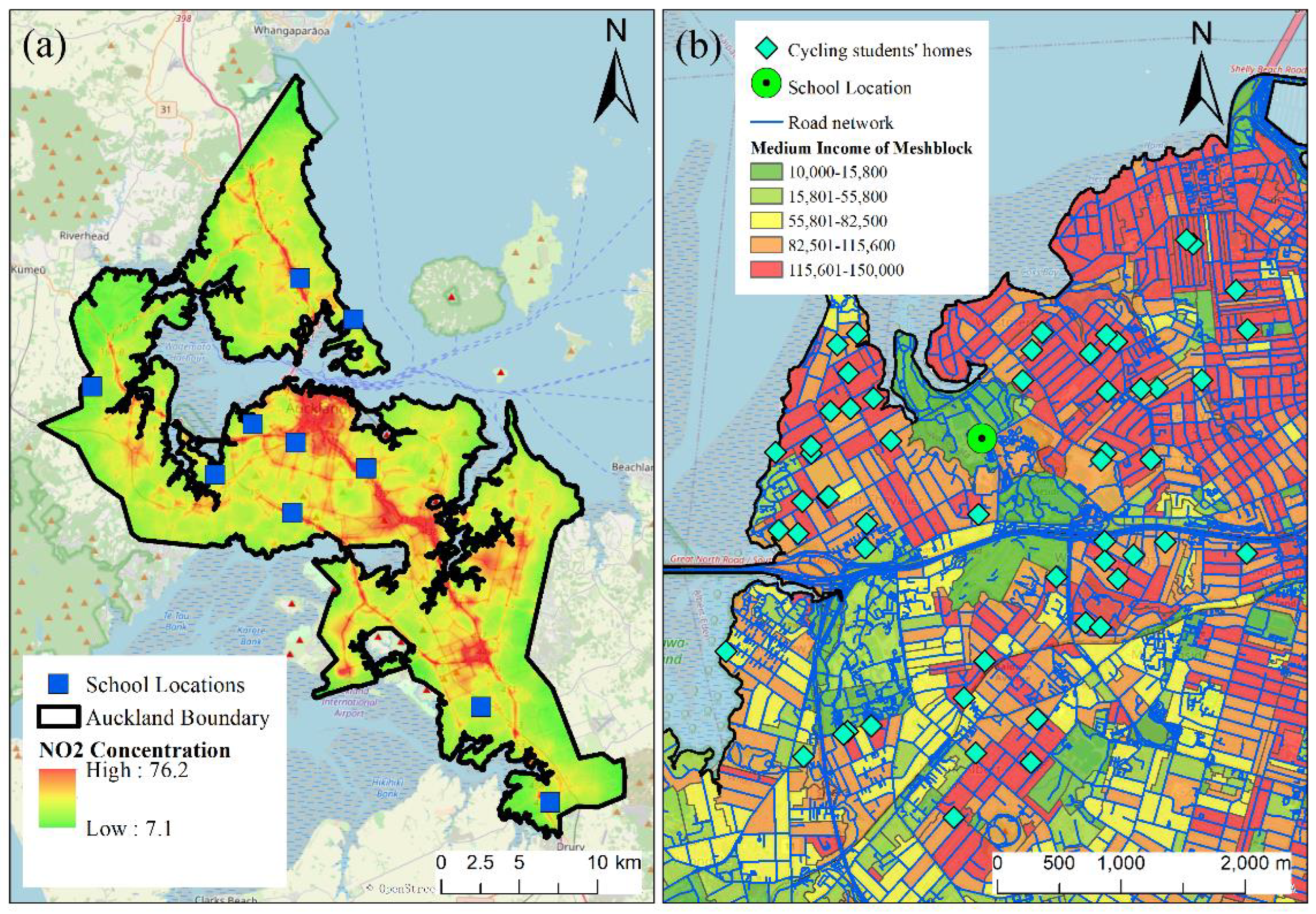
2.1. Study Area and Data Used

We choose Auckland as the study area since it is the largest and most populous city in New Zealand [15]. Auckland has a volcanic topography, and the terrain is hilly [1,15]. Air quality in Auckland is relatively good compared with that in cities in developing countries, but in recent years, with the increase in population and number of private vehicles, traffic-related air pollution (TRAP) has inevitably become a serious issue [16]. NO₂ is identified as an indicator for TRAP and has been widely used in previous studies [17,18,19]. Therefore, in this study, students’ dosage of NO₂ during cycling from home to school was investigated.

Cycling students’ information (e.g., home address and the school attended) was derived from the ‘Travelwise’ database. The intention and details of the ‘Travelwise’ project undertaken by Auckland Transport (AT) can be found in documents [1,20]. According to the statistical analysis of the ‘Travelwise’ data, among all survey samples, only 2.61% of students are cycling commuters. We randomly selected 10 high schools and intermediate schools (primary students are less likely to bike to school at a young age due to safety concerns) across Auckland to study 332 cycling students’ air pollution exposure during their daily commute from home to school.

Table 1. General information of schools involved in the study.

No.	School Name	Type of School	Location	No. of Cycling Students
1	Western Spring College	High School	Central Auckland	58
2	Mount Roskill Grammar School	High School	Central Auckland	20
3	Rosehill College	High School	South Auckland	8
4	Westlake Boys High School	High School	North Auckland	31
5	Takapuna Grammar School	High School	North Auckland	107
6	Massey High School	High School	West Auckland	16
7	Avondale College	High School	West Auckland	19
8	Kōwhai Intermediate School	Intermediate School	Central Auckland	19
9	Remuera Intermediate School	Intermediate School	Central Auckland	47
10	Manurewa Intermediate School	Intermediate School	South Auckland	7

shows the general information of the 10 schools and the number of cycling students in each school. Figure 1a shows the locations of the 10 schools on the map, and Figure 1b is an example demonstrating the location of a school and the cycling students’ home addresses.

2.2. Modeling Ambient NO₂ Concentration

In this study, we used the LUR approach to estimate spatial variations of NO₂ in Auckland. LUR models construct mathematical relationships between air pollution measurements and selected predictor variables reflecting driving factors of surrounding geographic features. Then, they can be used for prediction at unobserved locations. The LUR model developed by Ma et al. (2019) in study [15] was used in our study to estimate ambient NO₂ concentrations in the study area. Briefly, this model was developed based on annual NO₂ observations collected by 107 sites of passive samplers across Auckland (34, 30, and 43 sites in CBD, urban, and suburban, respectively). In the model development, more than 150 potential predictor variables were considered, and the supervised forward stepwise regression method proposed in the ESCAPE project was used to construct the model [16]. The authors report that the model had an R² of 0.68, 0.90, and 0.79 at the CBD, urban, and suburban, respectively. Then, this model was further rescaled (the rescaling approach can be found in the study [1]) for estimating annual mean NO₂ concentrations during morning peak hours (7:00−9:00 a.m.) as students’ cycling from home to school usually occurs during this time.

2.3. Determine the Cycling Network

A road network layer downloaded from the Auckland Transport website was used in this study to determine the cycling network. In the layer shapefile, there are more than 60,000 line features that can be categorized into 16 groups, such as motorways, major roads, and footpaths. Since this study only considered cycling commutes, motorway, motorway links, and train tracks were excluded from the network layer. The local trails and footpaths going through parks and open spaces were included in the network as cyclists are usually allowed to traverse them. ArcGIS 10.5 was used to form a redesigned cycling network for the subsequent procedures: (1) the entire network was segmented at crossings, converting each road feature into several line segments; (2) if any segment was longer than 20 m, it was then divided into several 20 m sub-segments.

2.4. Determine the Terrain-Based Dosage

Auckland’s hilly topography leads to dramatic variations in cycling speed and ventilation rate with changes in travel gradients [21,22]. Therefore, in this study, we developed a method to estimate the terrain-based respiratory dosage of air pollution during cycling along a certain route that accounts for variable cycling speed and ventilation rate related to topography. In brief, a commute route was split into several 20 m-interval road segments, and NO₂ concentration at each segment was estimated by the LUR model. The workflow for estimating NO₂ dosage while traversing each road segment is explained below.

Step 1: calculate gradient-related cycling speed for the road segment:

$$slopefacto{r}_{(s,l)}=\{\begin{array}{cc}1.5& \Leftarrow s<-30\\ 1+2\times \frac{0.7}{13}\times s+\frac{0.7}{{13}^2}\times s^2& \Leftarrow -30\le s<0\\ 1+{(\frac{s}{g(s,l)})}^2& \Leftarrow 0\le s\le 20\\ 10& \Leftarrow s>20\end{array}$$

(1)

$$g(s,l)=\{\begin{array}{cc}4& \Leftarrow 10<s\le 13\begin{array}{c}\end{array} \wedge \begin{array}{c}\end{array}l>15\\ 4.5& \Leftarrow 8<s\le 10\begin{array}{c}\end{array} \wedge \begin{array}{c}\end{array}l>30\\ 5& \Leftarrow 5<s\le 8\begin{array}{c}\end{array} \wedge \begin{array}{c}\end{array}l>60\\ 6& \Leftarrow 3<s\le 5\begin{array}{c}\end{array} \wedge \begin{array}{c}\end{array}l>120\\ 7& \Leftarrow otherwise\end{array}$$

(2)

$$slopefacto{r}_{(s,l)}^{adjst}=\{\begin{array}{c}10\Leftarrow s>13\begin{array}{c}\end{array} \wedge \begin{array}{c}\end{array}l>15\\ 10\Leftarrow s>10\begin{array}{c}\end{array} \wedge \begin{array}{c}\end{array}l>30\\ 10\Leftarrow s>8\begin{array}{c}\end{array} \wedge \begin{array}{c}\end{array}l>60\\ 10\Leftarrow s>5\begin{array}{c}\end{array} \wedge \begin{array}{c}\end{array}l>120\end{array}$$

(3)

To obtain gradient-related cycling speed, we need to first calculate a slope factor, which is determined by the slope and length of the road segment traversed [23]. In Equations (1)–(3), where s represents the direction-related slope of the road segment, expressed in %; l represents the length of the road segment (unit: m). By extracting elevations from the two endpoints of the segment, the slope can be calculated for each road segment.

$$v=\frac{v_{flat}}{slopefactor}$$

(4)

We assume a constant flat speed of 15 km/h for all cycling students, and the gradient-related cycling speed v can be calculated through Equation (4).

Step 2: calculate energy expenditure related to cycling speed, gradient, and gross mass of the cycling student:

$$W=\frac{v}{{\eta }_{mech}}\left[Mg\left(C_r+\frac{s}{100}\right)+0.5C_{D}A\rho {(v+C_w)}^2\right]$$

(5)

$$E_w=V{O}_2=450.00+9.7067\times W$$

(6)

First, the output power of cycling (W) is calculated using Equation (5), where M, g, ${\eta }_{mech}$, $C_r$, $C_D$, A, $\rho$, $C_w$ are the gross mass (bicycle + student), gravitational acceleration, mechanical efficiency of the bicycle, rolling resistance coefficient, aerodynamic drag coefficient, frontal area (bicycle + student), the density of air, and headwind; for simplicity, standard values used in other relevant studies are also applied in our study, and they are assumed to be 75 (15 + 60) kg, 9.81 m/s², 95%, 0.008, 1.2, 0.616 m², 1.226 kg/m³, and 0 m/s, respectively [24,25]. Second, the energy expenditure ($E_w$) or oxygen consumption rate (VO₂) is calculated using Equation (6). It is noticed that the VO₂ here is a relative VO_2, and the unit is mL/(kg·min). We need to convert it to an absolute VO₂ (unit: L/min) for later use [26].

Step 3: calculate ventilation rate $V_e$ (unit: L/min) based on energy expenditure $E_w$ (unit: L/min) obtained from Step 2 [27]:

$$\ln \frac{V_e}{M}=4.4329+1.0864\cdot \ln \frac{E_W}{M}-0.2829\cdot \ln A+0.0513X+\epsilon$$

(7)

where A is the age of the student (average age of 14 was used); $\epsilon$ obeys N (0, 0.1444). As the sex (X, male = 1 and female = 0) was unknown, the ventilation rate was calculated by averaging results derived from a male student and a female student, respectively.

Step 4: Determine the dosage (D_seg) while traversing the road segment:

$$D_{seg}=\frac{L_{seg}}{v}\times C_{N{O}_2}\times V_e$$

(8)

where $L_{seg}$ is the length of the road segment (20 m), $C_{N{O}_2}$ denotes the NO₂ concentration at the center of the road segment estimated by the LUR model. The total dose of a route can be calculated by summing the dosage in all road segments along the route.

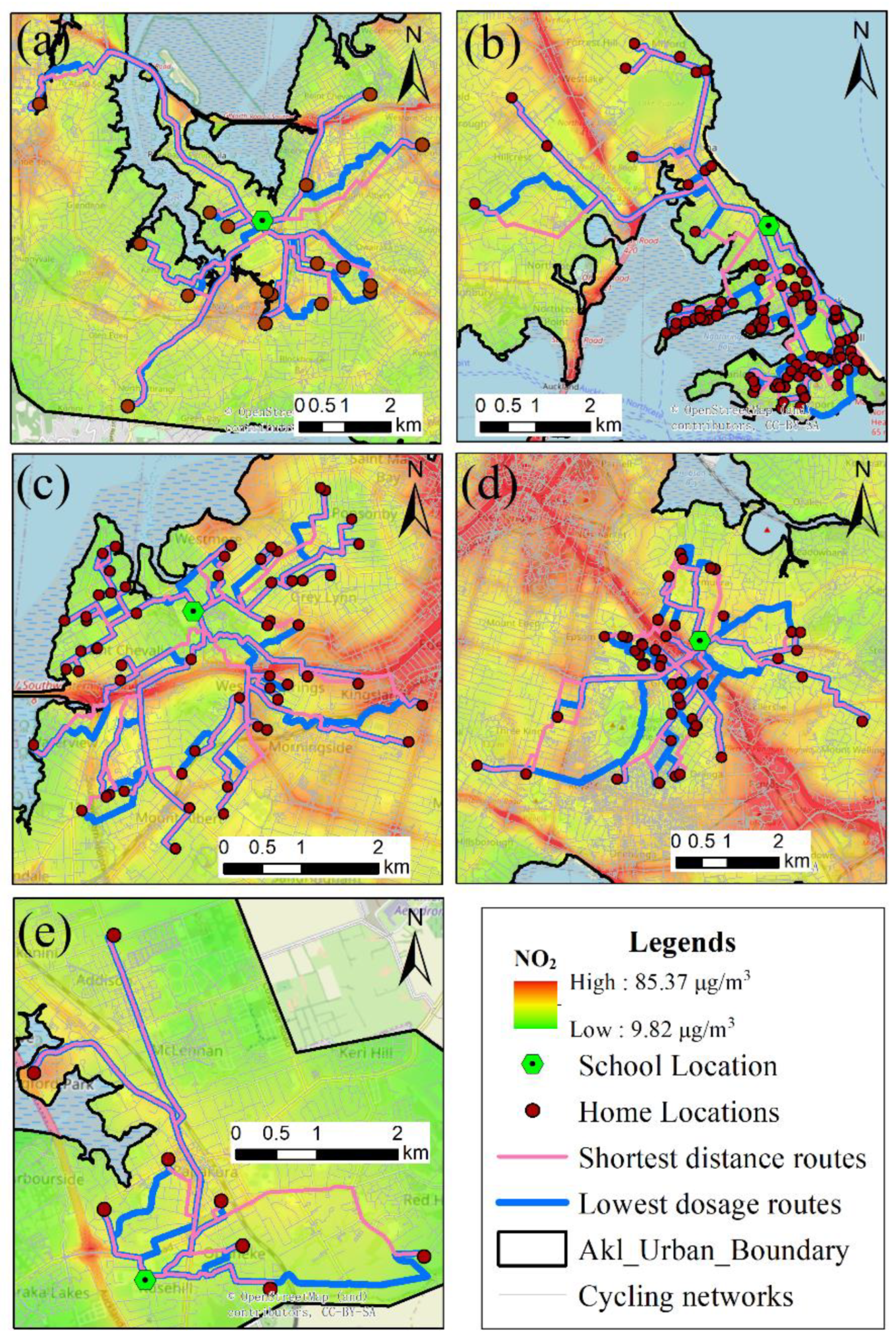
2.5. Spatial Analysis and Route Generation

To investigate students’ air pollution exposure in different commute route choices, two kinds of cycling routes from home to school (the shortest-distance and the lowest-dose routes) were generated for each student using road network analysis in ArcGIS 10.5. The shortest-distance route was studied as it is most students’ preference during the home-school commute [1]. The lowest-dose route (with the least cumulative dosage) was studied as it is an alternative route to reduce the exposure risk. The configuration of the network analysis was set as follows: (1) universal connectivity was selected since the network had been modified for cycling travel; (2) no restrictions were set for turning and one-way; (3) to consider the pollution inhaled during waiting for traffic signals at road crossings, cost barrier functions were applied in the dosage estimations (e.g., 40 s of the wait at a major crossing and 20 s at a minor crossing, both at a resting ventilation rate of 6 L·min⁻¹ [1]); (4) length and dosage were selected as impedances, respectively; and (5) they were also selected as accumulation attributes. The output of the road network analysis included: the origin, destination, total route length, and total NO₂ dosage for each home-school route. Given that some students may not be willing to use the alternative lowest-dose route if it were disproportionately longer, a restriction was set up to allow for the additional cycling distance up to 1000 m.

2.6. Exposure Justice during Cycling

Exposure justice (EJ) was also studied to examine the hypotheses: (1) cycling students from families of higher socioeconomic status are associated with a lower level of air pollution exposure, and (2) cycling students from families of lower socioeconomic status are associated with a higher level of air pollution exposure. In this study, cycling students’ socioeconomic status was represented by annual family income. In brief, each student’s annual family income value was extracted from a meshblock-level median annual family income map of Auckland (Figure 1b), and more details can be found in the study [1]. The annual family income values ranged from 10,000 to 150,000 NZD and, therefore, 80,000 NZD per annum was used as the determination between low (10,000–80,000) and high (80,000–150,000) levels of income. To fairly compare students’ exposure levels on different routes, the Unit Dosage Index (UDI) was introduced to represent the dosage someone inhaled per meter traversed and calculated by dividing the total dosage by the route length. Previous studies have identified that most students prefer to select the shortest-distance route for their home-school cycling commutes. Therefore, UDIs were derived for the 332 cycling students studied based on their shortest-distance routes between home and school. The median value of all UDIs was used as a determination to group the students with higher exposure (anyone’s UDI > the median value was determined as a higher exposure case). From the perspective of socioeconomic status, all cycling students were categorized into two groups (lower/higher income) based on their annual family incomes; from the perspective of exposure risks, all cycling students were also categorized into two groups (lower/higher exposure) based on their calculated UDIs. The portion of students at each income level and each exposure level were calculated, respectively. Then, the portion of students at the higher (lower) income level was compared accordingly with the portion of higher exposure students from the higher (lower) income level group to test the predefined hypothesis. All statistical results were calculated using R (version 3.3.0).

3. Results and Discussion

3.1. Descriptive Statistics

The highest, lowest, and mean NO₂ concentrations of the pollution map derived from the rescaled LUR model (adjusted to morning peak hours 7:00–9:00 a.m.) were 85.37 μg·m⁻³, 9.82 μg·m⁻³, and 25.64 μg·m⁻³, respectively. For the cycling network, there were altogether 535,327 features (road segments). The terrain-based slope of each road segment was derived by dividing the rise (the height of the slope) by the run (the distance of the slope), and the percentage of the slope was obtained by multiplying 100. This resulted in travel gradients of the cycling network ranging from −24.80% to +24.80%. The gradient-related cycling speed (a flat speed of 15 km/h was assumed) varied from 1.30 km/h (0.36 m/s) to 50.00 km/h (13.89 m/s) with the mean value of 17.51 km/h (4.82 m/s). The modeled energy expenditures varied from 0.45 L O₂/min to 1.75 L O₂/min. The varying ventilation rates were distributed around a mean of 12.02 L/min with a maximum value of 20.41 L/min (i.e., riding uphill with a steep slope) and a minimum value of 6.00 L/min (i.e., waiting at the road crossing).

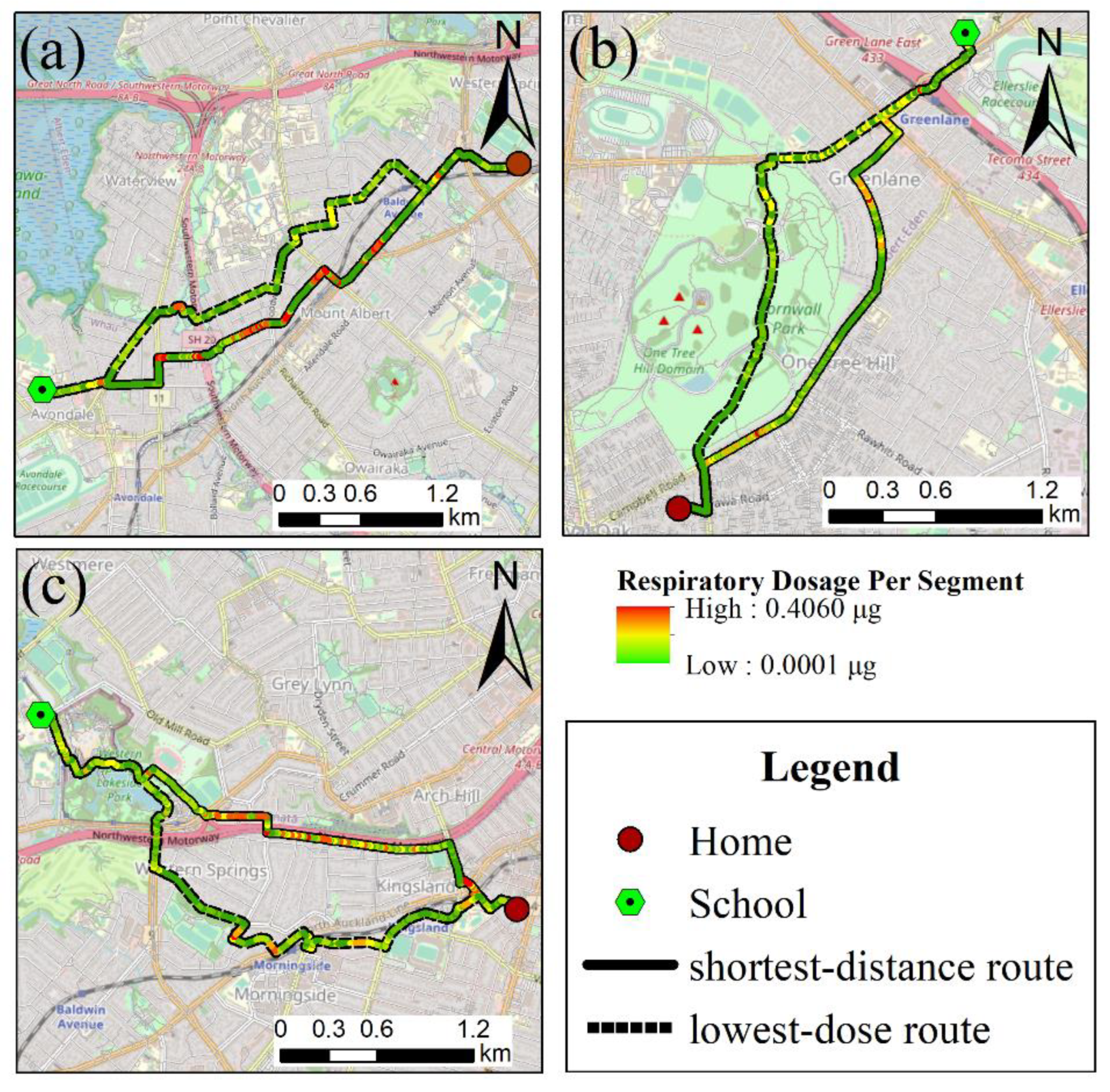
3.2. Dosage during Cycling Commutes along Different Routes

For all of the 332 cycling students in the 10 schools, we modeled and estimated their inhaled NO₂ dosage during commutes from home to school along with (a) the shortest-distance route and (b) the lowest-dosage route. Figure 2 visualizes and demonstrates different route choices (shortest distance vs. lowest dose) for each student in the school of (a) Avondale College; (b) Takapuna Grammar School; (c) Western Spring College; (d) Remuera Intermediate School; (e) Rosehill College.

Table 2. Statistical results for all students cycling along different routes.

Route Types	Statistics	Length (m)	Dosage (μg)
All shortest-distance routes	Max	8814.40	13.38
	Min	707.60	0.79
	Mean	2666.88	4.08
	Std	1162.08	2.04
All lowest-dose routes	Max	8865.34	13.25
	Min	707.60	0.79
	Mean	2837.17	3.82
	Std	1272.36	1.89
Alternative lowest-dose routes (those differ from their shortest-distance routes)	Max	8865.34	13.25
	Min	824.33	1.13
	Mean	3072.63	4.05
	Std	1258.39	1.91

shows the statistical results of route length and inhaled dosage for all 332 students cycling along different routes. The mean dosage was 4.08 and 3.82 μg per trip for the shortest-distance and lowest-dose routes, respectively. Accordingly, the mean route length for the two route choices was 2666.88 and 2837.17 m, respectively. On average, one cycling student could reduce 6.37% of NO₂ dosage with 6.39% additional route length if a lowest-dose route was used during the home-school commute. For any home-school pair (one sample of a cycling student), its lowest-dosage route is identified as an alternative lowest-dosage route (ALDR) if it is different from its corresponding shortest-distance route.

As the goal of our study was to examine the potential for air pollution exposure reduction if students use alternative cleaner routes during daily school commutes, we analyzed all ALDRs and compared them with the corresponding shortest-distance route in more depth.

Table 3. The proportion of ALDRs found for students in each school.

No.	School Name	No. of Students	No. of ALDRs	Proportion
1	Western Spring College	58	45	77.59%
2	Mount Roskill Grammar School	20	15	75.00%
3	Rosehill College	8	6	75.00%
4	Westlake Boys High School	31	22	70.97%
5	Takapuna Grammar School	107	87	81.31%
6	Massey High School	16	10	62.50%
7	Avondale College	19	13	68.42%
8	Kōwhai Intermediate School	19	17	89.47%
9	Remuera Intermediate School	47	38	80.85%
10	Manurewa Intermediate School	7	2	28.57%
Sum		332	255	76.81%

shows the proportion of ALDRs found for students in each school. Varying from 28.57% to 89.47% between schools, the general proportion was 76.81%. These results indicate that most students could find an alternative, cleaner route (e.g., ALDR) during their daily commute from home to school that differs from the routine shortest-distance route. The factors that determine the proportion of ALDRs found for students in each school may include: (1) the connectivity of the road network around a school, (2) the variations of travel gradients of the road network around a school, (3) the variations of air pollutant concentrations in the region around a school, and (4) the distance between home and the school. Kōwhai Intermediate School had the highest proportion of 89.47% among the 10 investigated schools due to its location in central Auckland (near the central business district). On the one hand, the road network connectivity in this area is significantly better than that of other places (the road network in suburban Auckland was largely designed after 1950 mostly for private vehicles), and a network with better connectivity tends to have a higher chance to find an alternative route between home and school; on the other hand, the central Auckland is a relatively heavily polluted area with large spatial gradients of air pollutant concentrations varying between streets and this also makes it easier to form an alternative cleaner route. Takapuna Grammar School had the second highest proportion of 81.31% among them, probably due to distinct spatial variations of terrain gradients around the school. In the North Head region (lower right of Figure 2b), its volcanic topography is generally hilly, and cycling speeds, energy expenditure, and ventilation rates tend to vary dramatically between different road segments. This makes it easy to form an ALDR. Manurewa Intermediate School had the lowest proportion of 28.57%, largely due to the short distance between students’ homes and the school. The mean length of the shortest-distance route for those students is 1867.52 m, which is 29.97% shorter than the mean route length of all the students (2666.88 m). As we know, it is less likely to have an alternative route for a short trip.

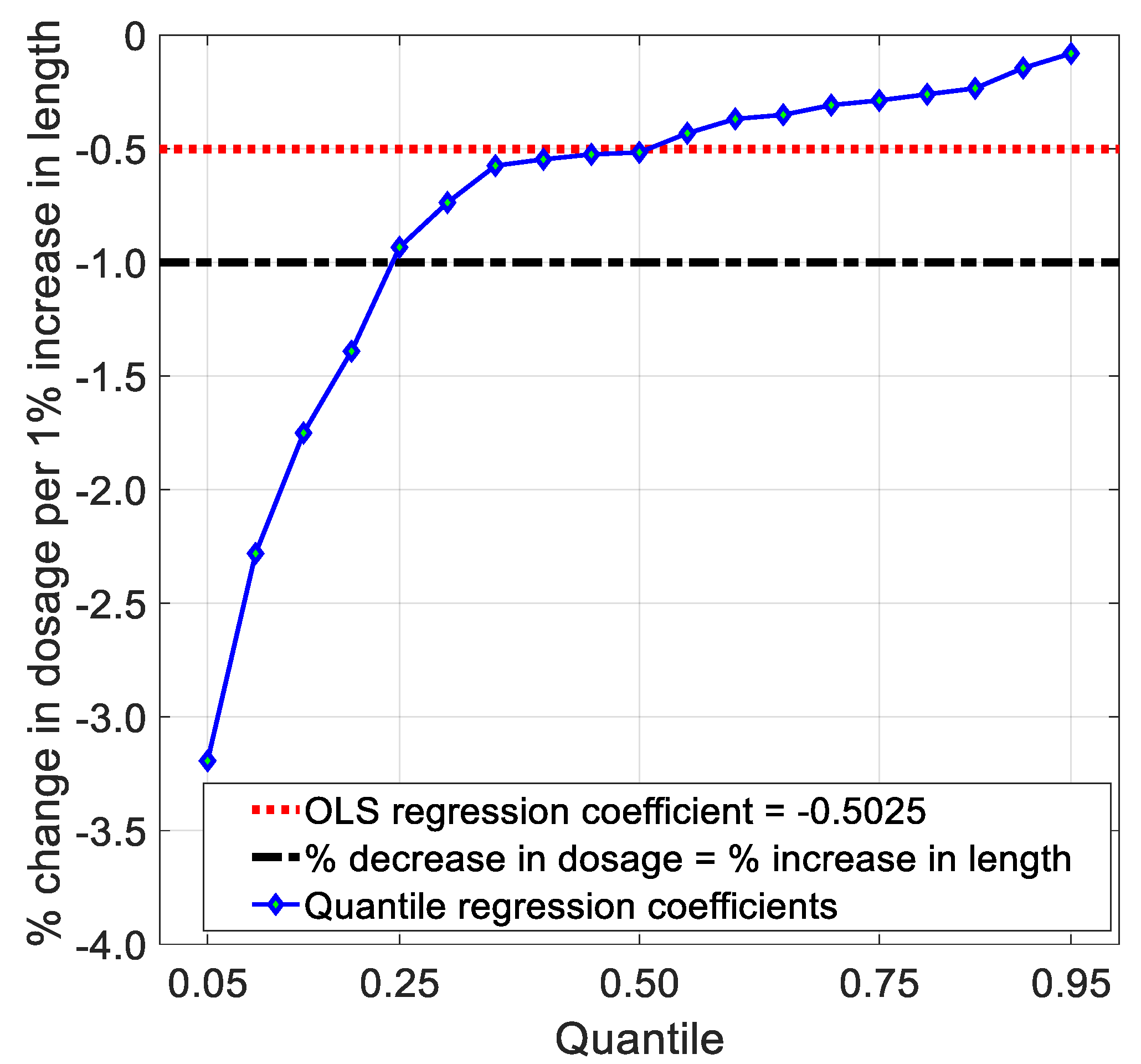
3.3. Trade-Off between Different Route Choices

The trade-off between different route choices (the routine shortest-distance route vs. ALDR) was analyzed for those 255 students that had ALDRs from home to school. Figure 3 shows the scatterplot of relative change in route length (expressed in %) vs. relative change in dosage (expressed in %) for the studied 255 samples (the red squares).

Averagely, ALDRs (3072.63 m) were 7.78% longer than their corresponding shortest-distance route (2850.92 m) in terms of mean route length, and the mean NO₂ dosage of ALDRs (4.06 μg) was 7.79% lower than that of its counterpart (4.40 μg). Statistically, the benefit (e.g., reducing inhaled NO₂ dose) of using an ALDR equaled (or marginally outweighed) the corresponding cost (e.g., riding more route length). However, the regression line (blue) in Figure 3 was on the right side of the 1:1 line (black), which indicates that for a large part of students 1% decrease in NO₂ dosage was associated with a more than 1% increase in route length from the perspective of a scatter plot. To further investigate the trade-off between these two route choices, quantile regression for the 255 samples was carried out to illustrate the conditional quantiles of relative change in dosage as a linear function of per 1% increase in route length. Figure 4 shows the quantile regression plot of relative change in dosage per 1% increase in route length. Generally, the cost significantly outweighed the benefit for most individuals. For example, for 50% of ALDRs, a 1% increase in route length was associated with only a 0.50% decrease in NO₂ dosage. In other words, the relative decrease in dosage of riding along an ALDR was smaller than the relative increase in route length. However, for many students, using an ALDR also had a positive side as for 20% (15%, 10%, 5%) of the routes, a 1% increase in route length was associated with a > 1.4% (1.7%, 2.3%, 3.2%) decrease in NO₂ dosage. For example, in Figure 3, a cycling student achieved a 26.47% reduction in NO₂ dosage with riding only a 2.91% additional route length.

3.4. Exposure (In)Justice

EJ during students’ cycling from home to school was also studied in this study.

Table 4. The portion of students from an income level vs. their portion of a higher UDI.

Income Level	Income Ranges	Population Proportion	High Exposure Proportion
Low income	10–80 K	24.10%	27.11%
High income	80–150 K	75.90%	72.89%

shows the portion of students from an income level vs. their portion of a higher UDI. Among all 332 students, 80 and 252 students were from families of low income and high income, which took up 24.10% and 75.90% of the whole sample, respectively. While in the 166 students of high exposure cases (with a higher UDI), 45 and 121 students were from families of low income and high income, which took up 27.11% and 72.89% of the high exposure group, respectively. In other words, students from families of low income accounted for 24.10% of the population, but they contributed 27.11% (>24.10%) of high exposure cases (bold fonts were used to emphasize the fact that the high exposure proportion was higher than the population proportion in Table 4). This indicates that cycling students from families of lower socioeconomic status are associated with a higher level of air pollution exposure. In contrast, students from families of high income accounted for 75.90% of the population, but they only contributed 72.89% (<75.90%) of high exposure cases. This indicates that cycling students from families of higher socioeconomic status are associated with a lower level of air pollution exposure. These results verified the existence of exposure injustices (or exposure inequalities) during students’ cycling from home to school.

3.5. General Discussion

In this study, we modeled students’ terrain-based dosage of ambient NO₂ during cycling from home to school for the very first time and further compared the benefit and costs of different route choices. Moreover, EJ during students’ cycling commutes was examined as well.

A few previous studies also estimated cyclists’ dose of air pollution during daily cycling commutes. Studies [12,13,14] estimated cyclists’ dosages of particulate matter, NO₂, CO, and SO_2, using different modeling frameworks. However, a common shortcoming in these studies is that they both assumed a fixed ventilation rate in the dose estimation, as, in reality, nobody rides a bicycle at a fixed speed with a constant inhale rate. The study [28] improved this issue by introducing the term heart rate in the equation to estimate the dynamic ventilation rate during the route as one’s ventilation rate is dependent on physical activities, and the heart rate can be physiologically linked to ventilation. However, this method requires the direct measure of each cyclist’s heart rate during his/her cycling commutes. Therefore, this approach cannot be applied to estimate cyclists’ dose of air pollution during commutes on a population scale. The modeling framework proposed in our study is based on the assumption that riding speed is associated with the varying terrain-related travel gradients and the dynamic energy expenditure, and ventilation rate is physiologically linked with the estimated gradient-related cycling speed. Finally, the estimated cyclist’s dose of air pollution can account for terrain-related riding speed, energy expenditure, and ventilation rate during the route. Logically, our approach could be applied to estimate cyclists’ dose of any air pollutant at a population scale in any other study area as long as the air pollutant concentration map, terrain information, and road network data are provided.

In our study, 76.81% of cycling students can find an ALDR. This proportion is significantly higher than that of the 17.48% found in a previous study also conducted in Auckland that focused on students’ dose of NO₂ while walking from home to school [1]. This difference and the higher proportion in our study could be caused by two reasons: (1) in general, cycling students (2667 m) had a longer commute distance than walking students (1129 m), and as aforementioned analysis, a longer trip tends to have more chance to find an ALDR; (2) the range and variation of ventilation rate during cycling (6.0–20.4 L/min) is greater than walking (6.0–17.3 L/min), and this could also increase the chance of generating an ALDR. In joint consideration of statistics of the mean dosage of cycling (4.08 μg) and walking (6.36 μg) commutes in these two studies, cyclists tend to inhale less dose of NO₂ during home-school commutes. This founding is consistent with the result of a previous case study conducted in Hamilton, Ontario, Canada [29].

Previous studies [30,31,32,33] have identified the existence of exposure inequalities in students’ homes and at school. Our study further explored cycling students’ EJ issues during their riding from home to school, and the results demonstrate that exposure inequalities existed to some extent during cycling commutes. Further studies are needed to explore the pathway to mitigate the inequalities.

The findings in this study could deepen our understanding of cycling students’ exposure to air pollution and provide scientific advice for policymakers to optimize students’ daily active commuting routes. Some recommendations include: (1) for active commuting, cycling tends to be a better option as it results in a significantly lower dose of air pollution than walking; (2) for a short trip, cycling students can simply use the shortest-distance route to school; (3) for a long trip, cycling students could try to find an ALDR if benefit beat cost; (4) as shown in Figure 5, an ALDR could be found by riding along a local road parallel with or a pathway in the park/greenspace close to the major road, or using a distant less-polluted road parallel with the heavily polluted motorway.

4. Conclusions

The commuting activities account for a disproportionately high amount of people’s total diurnal exposure. Accurate measuring of students’ dose of air pollution during their daily commutes could advance our knowledge of mitigating the adverse effect of exposure to air pollution. In this study, we proposed a modeling framework to estimate cycling students’ terrain-based dosage of ambient NO₂ during home-school commutes for the very first time and further compared the benefit and costs of different route choices. Our study advances in the relevant field as it accounts for terrain-related riding speed, energy expenditure, and ventilation rate; furthermore, the approach is scalable and applicable to any other place where required data exist. The results show that for parts of cycling students, they can find an ALDR to reduce the inhaled dose of air pollution with a sacrifice of riding cost-effectively additional route lengths. The findings in our study could deepen our understanding of cyclists’ exposure and provide scientific advice for policymakers to optimize students’ daily active commute routes. The limitations of our study include: (1) we used averaged values for parameters (e.g., age, weight, etc.) in the estimation of each student’s energy expenditure and ventilation rate, the accuracy of this estimation can be further improved if the exact values are known; (2) we used the shortest-distance route from home to school as a surrogate of a student’s real home-school commute route, this may also introduce biases and uncertainties into the analysis. In future work, we could compare the results generated based on modeling with direct measurements to further assess the accuracy of our approach. Our study suggests that local governments could mitigate the adverse health effects of students’ exposure to air pollution during commuting by (1) developing an online website or smartphone APP to optimize students’ commute routes in a short-term view; (2) considering reduction in air pollution exposure in future urban construction planning in a long-term view.

References

1. Ma, X.; Longley, I.; Gao, J.; Salmond, J. Evaluating the Effect of Ambient Concentrations, Route Choices, and Environmental (in) Justice on Students’ Dose of Ambient NO2 While Walking to School at Population Scales. Environ. Sci. Technol. 2020, 54, 12908–12919. [Google Scholar] [CrossRef]
2. Dominski, F.H.; Branco, J.H.L.; Buonanno, G.; Stabile, L.; da Silva, M.G.; Andrade, A. Effects of Air Pollution on Health: A Mapping Review of Systematic Reviews and Meta-analyses. Environ. Res. 2021, 201, 111487. [Google Scholar] [CrossRef]
3. Alvarez-Pedrerol, M.; Rivas, I.; López-Vicente, M.; Suades-González, E.; Donaire-Gonzalez, D.; Cirach, M.; de Castro, M.; Esnaola, M.; Basagaña, X.; Dadvand, P.; et al. Impact of Commuting Exposure to Traffic-related Air Pollution on Cognitive Development in Children Walking to School. Environ. Pollut. 2017, 231, 837–844. [Google Scholar] [CrossRef] [Green Version]
4. Engström, E.; Forsberg, B. Health Impacts of Active Commuters’ Exposure to Traffic-related Air Pollution in Stockholm, Sweden. J. Transp. Health 2019, 14, 100601. [Google Scholar] [CrossRef]
5. Rivas, I.; Donaire-Gonzalez, D.; Bouso, L.; Esnaola, M.; Pandolfi, M.; De Castro, M.; Viana, M.; Àlvarez-Pedrerol, M.; Nieuwenhuijsen, M.; Alastuey, A.; et al. Spatiotemporally Resolved Black Carbon Concentration, Schoolchildren’s Exposure and Dose in Barcelona. Indoor Air. 2016, 26, 391–402. [Google Scholar] [CrossRef] [Green Version]
6. Buonanno, G.; Giovinco, G.; Morawska, L.; Stabile, L. Tracheobronchial and Alveolar Dose of Submicrometer Particles for Different Population Age Groups in Italy. Atmos. Environ. 2011, 45, 6216–6224. [Google Scholar] [CrossRef] [Green Version]
7. Paunescu, A.C.; Attoui, M.; Bouallala, S.; Sunyer, J.; Momas, I. Personal Measurement of Exposure to Black Carbon and Ultrafine Particles in Schoolchildren from PARIS Cohort (Paris, France). Indoor Air. 2017, 27, 766–779. [Google Scholar] [CrossRef]
8. Ma, X.; Longley, I.; Gao, J.; Salmond, J. Assessing Schoolchildren’s Exposure to Air Pollution during the Daily Commute-A Systematic Review. Sci. Total Environ. 2020, 737, 140389. [Google Scholar] [CrossRef]
9. Pujol, J.; Martínez-Vilavella, G.; Macià, D.; Fenoll, R.; Alvarez-Pedrerol, M.; Rivas, I.; Forns, J.; Blanco-Hinojo, L.; Capellades, J.; Querol, X.; et al. Traffic Pollution Exposure Is Associated with Altered Brain Connectivity in School Children. Neuroimage 2016, 129, 175–184. [Google Scholar] [CrossRef] [PubMed] [Green Version]
10. Tudor-Locke, C.; Ainsworth, B.E.; Popkin, B.M. Active Commuting to School. Sports Med. 2001, 31, 309–313. [Google Scholar] [CrossRef] [PubMed]
11. Gilliland, J.; Maltby, M.; Xu, X.; Luginaah, I.; Loebach, J.; Shah, T. Is Active Travel a Breath of Fresh Air? Examining Children’s Exposure to Air Pollution during The School Commute. Spat. Spatiotemporal Epidemiol. 2019, 29, 51–57. [Google Scholar] [CrossRef] [PubMed]
12. Carreras, H.; Ehrnsperger, L.; Klemm, O.; Paas, B. Cyclists’ Exposure to Air Pollution: In Situ Evaluation with a Cargo Bike Platform. Environ. Monit. Assess. 2020, 192, 470. [Google Scholar] [CrossRef] [PubMed]
13. Agarwal, A.; Kaddoura, I. On-road Air Pollution Exposure to Cyclists in an Agent-Based Simulation Framework. Period. Polytech. Transp. Eng. 2020, 48, 117–125. [Google Scholar] [CrossRef]
14. Adams, M.D.; Yiannakoulias, N.; Kanaroglou, P.S. Air Pollution Exposure: An Activity Pattern Approach for Active Transportation. Atmos. Environ. 2016, 140, 52–59. [Google Scholar] [CrossRef]
15. Ma, X.; Longley, I.; Gao, J.; Kachhara, A.; Salmond, J. A Site-optimised Multi-scale GIS Based Land Use Regression Model for Simulating Local Scale Patterns in Air Pollution. Sci. Total Environ. 2019, 685, 134–149. [Google Scholar] [PubMed]
16. NZ MfE. Emissions Inventories for CO, NOx, SO2, Ozone, Benzene and Benzo(a)pyrene in New Zealand. Available online: https://environment.govt.nz/publications/emission-inventories-for-co-nox-so2-ozone-benzene-and-benzoapyrene-in-new-zealand/ (accessed on 21 June 2022).
17. Weissert, L.F.; Salmond, J.A.; Miskell, G.; Alavi-Shoshtari, M.; Williams, D.E. Development of a Microscale Land Use Regression Model for Predicting NO2 Concentrations at a Heavy Trafficked Suburban Area in Auckland, NZ. Sci. Total Environ. 2018, 619–620, 112–119. [Google Scholar] [CrossRef]
18. Miskell, G.; Salmond, J.; Longley, I.; Dirks, K.N. A Novel Approach in Quantifying the Effect of Urban Design Features On Local-Scale Air Pollution in Central Urban Areas. Environ. Sci. Technol. 2015, 49, 9004–9011. [Google Scholar] [CrossRef]
19. Beelen, R.; Hoek, G.; Vienneau, D.; Eeftens, M.; Dimakopoulou, K.; Pedeli, X.; Tsai, M.Y.; Künzli, N.; Schikowski, T.; Marcon, A.; et al. Development of NO2 and NOx Land Use Regression Models for Estimating Air Pollution Exposure in 36 Study Areas in Europe–The ESCAPE Project. Atmos. Environ. 2013, 72, 10–23. [Google Scholar] [CrossRef]
20. Morton, T. Travelwise to School: Delivering School Travel Plans in The New Zealand Environment. In Proceedings of the Australasian Transport Research Forum (ATRF), Sydney, Australia, 28–30 September 2005. [Google Scholar]
21. Chieng, M.; Lai, H.; Woodward, A. How Dangerous Is Cycling in New Zealand? J. Transp. Health. 2017, 6, 23–28. [Google Scholar] [CrossRef]
22. Mirza, L.; Cheung, A.K.; Moradi, S. Understanding Factors Influencing Choices of Cyclists and Potential Cyclists: A Case Study at The University of Auckland. Road Transp. Res. 2014, 23, 37–51. [Google Scholar]
23. Price, M. Slopes, Sharp Turns, and Speed: Refining Emergency Response Networks to Accommodate Steep Slopes and Turn Rules. Hands On ArcUser Spring 2008, 11, 50–57. [Google Scholar]
24. Parkin, J.; Rotheram, J. Design Speeds and Acceleration Characteristics of Bicycle Traffic for Use in Planning, Design and Appraisal. Transport Pol. 2010, 17, 335–341. [Google Scholar] [CrossRef]
25. Liu, L.; Suzuki, T. Quantifying E-Bike Applicability by Comparing Travel Time and Physical Energy Expenditure: A Case Study of Japanese Cities. J. Transp. Health. 2019, 13, 150–163. [Google Scholar] [CrossRef]
26. Zoladz, J.A.; Rademaker, A.C.H.J.; Sargeant, A.J. Non-Linear Relationship Between O2 Uptake and Power Output at High Intensities of Exercise in Humans. J. Physiol. 1995, 488, 211–217. [Google Scholar] [CrossRef] [PubMed] [Green Version]
27. US EPA. Metabolically Derived Human Ventilation Rates: A Revised Approach Based upon Oxygen Consumption Rates. Available online: https://ordspub.epa.gov/ords/eims/eimscomm.getfile?p_download_id=490080 (accessed on 21 July 2022).
28. Hofman, J.; Samson, R.; Joosen, S.; Blust, R.; Lenaerts, S. Cyclist Exposure to Black Carbon, Ultrafine Particles and Heavy Metals: An Experimental Study Along Two Commuting Routes Near Antwerp, Belgium. Environ. Res. 2018, 164, 530–538. [Google Scholar] [CrossRef] [PubMed]
29. Adams, M.; Bennet, S.; Yiannakoulias, N.; Kanaroglou, P. Does Walking or Cycling Provide the Lowest PM2.5 Air Pollution Dose During the Trip from Home to School for Children? In Proceedings of the Canadian Transportation Research Forum, Windsor, ON, Canada, 1–4 June 2014. [Google Scholar]
30. Cakmak, S.; Hebbern, C.; Cakmak, J.D.; Vanos, J. The Modifying Effect of Socioeconomic Status on the Relationship Between Traffic, Air Pollution and Respiratory Health in Elementary Schoolchildren. J. Environ. Manage. 2016, 177, 1–8. [Google Scholar] [CrossRef] [Green Version]
31. Grineski, S.E.; Collins, T.W. Geographic and Social Disparities in Exposure to Air Neurotoxicants at US Public Schools. Environ. Res. 2018, 161, 580–587. [Google Scholar] [CrossRef]
32. Jephcote, C.; Chen, H. Environmental Injustices of Children’s Exposure to Air Pollution from Road-Transport Within the Model British Multicultural City of Leicester: 2000–2009. Sci. Total Environ. 2012, 414, 140–151. [Google Scholar] [CrossRef]
33. Chakraborty, J.; Zandbergen, P.A. Children at Risk: Measuring Racial/Ethnic Disparities in Potential Exposure to Air Pollution at School and Home. J. Epidemiol. Commun. Health 2007, 61, 1074–1079. [Google Scholar] [CrossRef]
Figure 1. Maps demonstrating the study area and cycling student samples: (a) locations of the 10 schools involved in the study and the map of annual ambient NO2 concentrations of Auckland; (b) an example showing the location of a school and the cycling students’ home addresses (Note: The legends were deliberately drawn at a rather large size to prevent the identification of the exact addresses).
Atmosphere 13 01612 g001
Figure 2. Visualization of route choices (shortest distance vs. lowest dose) for students in each school: (a) Avondale College; (b) Takapuna Grammar School; (c) Western Spring College; (d) Remuera Intermediate School; (e) Rosehill College.
Atmosphere 13 01612 g002
Figure 3. Scatterplot of relative change in route length vs. relative change in dosage.
Atmosphere 13 01612 g003
Figure 4. Quantile regression plot of relative change in dosage per 1% increase in route length.
Atmosphere 13 01612 g004
Figure 5. Examples illustrate the generation of the lowest-dose route compared with the routine shortest-distance route. (a) riding along a local road parallel with the major road; (b) using the pathway in a park or greenspace close to the major road; (c) using a distant less-polluted road parallel with the heavily polluted motorway.
Atmosphere 13 01612 g005