Article

Incremental Evaluation Model for the Analysis of Indoor Air Measurements

by
Andreas Schmohl
*,
Michael Buschhaus
,
Victor Norrefeldt
,
Sabine Johann
,
Andrea Burdack-Freitag
,
Christian R. Scherer
,
Pablo A. Vega Garcia
and
Christoph Schwitalla
Fraunhofer Institute for Building Physics IBP, Fraunhoferstr. 10, 83626 Valley, Germany
*
Author to whom correspondence should be addressed.
Atmosphere 2022, 13(10), 1655; https://doi.org/10.3390/atmos13101655
Submission received: 30 August 2022 / Revised: 30 September 2022 / Accepted: 5 October 2022 / Published: 11 October 2022

Abstract

:
The investigation of the cleaning effectiveness of air cleaners under realistic conditions is challenging. Mathematical models are needed to extract characteristic properties of the air cleaning system from experimental data. An incremental evaluation model based on a source term and a total first-order loss coefficient in each segment was developed to analyze indoor particle measurements. The application of the model is demonstrated using two scenarios, one in a well-mixed testing room and another in a fully equipped aircraft cabin at 750 hPa with a typical aircraft ventilation system. In the first scenario, a normalized version of the model is used to eliminate the source’s influence. For the investigation in the aircraft cabin, the model served to extract temporal and spatial resolved source terms and first-order loss coefficients. The incremental evaluation model is applicable to enhance the certification of air cleaners. The application of the model is not only limited to particles; measurements of gaseous compounds like ozone, carbon dioxide, or volatile organic compounds can be evaluated analogously. The model’s utility for the data analysis of experiments with complex flow conditions should be studied in further investigations.

1. Introduction

Air cleaners (AC) can remove particulate matter (PM) and bioaerosols from indoor air [1,2,3]. The concept of a virtual clean air delivery rate (CADR) is used to specify the cleaning efficiency of an air cleaner at a certain physical volume flow [2,3,4,5,6,7,8]. The cleaning efficiency depends on the type of matter that has to be removed from the indoor air. The contaminants could be particulate matter [1,2,3,8,9], volatile organic compounds [10], or inorganic gaseous compounds. Furthermore, in the case of particulate matter, the cleaning efficiency of an air cleaner depends on the particle size distribution [2,3,6].
The removal effectiveness of an air cleaner can be specified in a laboratory under controlled and reproducible conditions. Mathematical models can implement the analysis of the experimental data of the test. Without a source that releases matter in the analyzed phase of the experiment, a simple exponential decay function can be used for the analysis [2,4,5,6]. While matter is released or contaminated outdoor air is infiltrating the room, a source term has to be considered [11,12,13,14,15]. Models based on a source term and a first-order loss term are common and well described elsewhere [3,8,10,11,12,14,15,16,17,18].
The general purpose of a fitting function is to describe a set of data. Ideally, all used fitting parameters are related to a physical-chemical meaning. The focus of this research was the development and application of an incremental fitting model. The model should be based on an equation that describes each segment. Hence for each phase of the experiment, the concentration curve between the concentration at the beginning of each segment and the equilibrium concentration at infinity. An analogous equation was utilized by Schumacher et al. and Jung; however, Jung did not use the option to string together several segments to create an incremental evaluation model, and Schumacher et al. did not use the model for data analysis [3,12]. In the case of first-order kinetics, the equilibrium concentration in this model equals the source term divided by a first-order loss coefficient [3,12].
This research demonstrates the application of the incremental evaluation model using two scenarios. The first application scenario—“case study I”—is the determination of a clean air delivery rate (CADR) of a mobile air cleaner in a test room with well-mixed conditions. The second application scenario—“case study II”—investigates a non-thermal plasma air cleaning technology as an alternative technology for aircraft cabins. Generally, the feeding air in aircraft cabins is filtered by HEPA filters [9]. These filters are installed in the ventilation ducts. The advantage of the investigated alternative air cleaning technology was the reduction of the pressure drop in the ventilation duct resulting in lower energy consumption of the ventilation system. The flow conditions in aircraft cabins are complex; therefore, the temporal and spatial characteristics must be considered. When emitting particles in the aircraft cabin, measurements [19] and simulations [20] clearly show a spacial variation with increased concentrations closer to the emitter and lower concentrations farther away. This proves that the assumption of perfect mixing cannot be applied to such environments. Investigations in similar environments like train compartments similarly show that the distance from a virus emitter in the carriage is crucial for the exposure, and perfect mixing cannot be assumed [21,22]. Therefore, case study II focused on the temporal and spatial resolved evaluation of the source term s [(µg/m3)/h)] and total first-order loss coefficient k [h−1].
Applications of the incremental evaluation model for particulate matter, Phi6 bacteriophage bioaerosol, and ozone have recently been published [13,23].

2. Materials and Methods

2.1. Materials

Three identical light scattering aerosol spectrometers LSAS (Fidas Frog, Palas GmbH, Karlsruhe, Germany) were used to measure the aerosols in a micro range of 0.18–20 µm. The aerosol spectrometers continuously recorded PM fractions (PM1, PM2.5, and PM10) and the particle number concentration.
A nebulizer (AGK 2000, Palas GmbH, Karlsruhe, Germany) nebulized an aerosol at 1.5 bar inlet pressure into the room air. The nebulized liquid was a Phi 6 (Pseudomonas Phage Phi6; DSM 21518) bacteriophage suspension, according to AHAM AC-5-2022 [24]. The molar concentrations of the salts in the suspension were: 86 mM NaCl, 49 mM Na2HPO4, 22 mM KH2PO4, 1 mM CaCl2, and 1 mM MgSO4.
The microbiological analysis is not relevant to this publication. However, microbiological sampling is described hereafter because the air sampling influenced the particle measurements (see Section 3.2.6). For the microbiological analysis, a bacteriophage plaque assay was used [23,25]. The plaque assay proceeded according to DIN EN 13610 [26]. Air samples for the plaque assays were collected with an airflow of 3 m3/h by a Holbach air sampler (MBASS30V3, Umweltanalytik Holbach GmbH, Wadern, Germany).

2.2. Test Room for Determination of Clean Air Delivery Rate (CADR)

The air cleaner test was conducted in the Fraunhofer Indoor Air Test Center (IATC) in Valley, Germany (Figure 1). The IATC is a test facility with a room volume of 129 m3 (8.24 × 5.06 × 3.09 m3), where the climatic conditions are specifically set and kept constant over the measurement period. The test room was equipped with chairs and tables to simulate the situation in a classroom or an office.
The nebulizer continuously nebulized the phage suspension into the air. The aerosol spectrometers continuously recorded PM fractions in addition to the particle number concentration (or particle count, respectively) at three different positions in the room. Two fans, each with a volume flow of 400 m3/h and directed against each other, mixed the air during the entire test procedure. One fan was placed behind the aerosol generator, and the second in front of the air cleaner (see Figure 1b). The test procedure was subdivided into five phases, see Table 1.

2.3. Investigation of an Air Cleaner in an Aircraft Cabin

The Fraunhofer Flight Test Facility (FTF) is a test platform on which aircraft ventilation systems and the tracing of in-cabin transmission can be investigated. In addition, real emission data can be used to evaluate various air cleaning devices. The full-size demonstrator consists of a front section of a long-range twin-aisle aircraft with ten rows of 2/4/2 seating (Figure 2). It has original ceiling air inlets, lateral inlets below the overhead bins, and extraction below the side wall at floor level into the triangle area (cheeks). Here the airflow is split into recirculation and exhaust air extracted from the bilge section. The aircraft’s cabin volume is 107 m3.
The experimental schedule and the documented events are listed in Table 2. The cleaning technology was implemented in the recirculation line. State of the art uses HEPA filters to purify the cabin air. In this test setup, the air in the recirculation line was first cleaned by a HEPA filter. Afterwards, the HEPA filter was removed and replaced by a non-thermal plasma air cleaner.
The experimental setup followed a scenario with a continuous emitter in the cabin, simulating the continuous exhalation of aerosols. The aerosol release was realized by a modified “breathing” Sheffield head which was combined with the aerosol generator and placed at seat number 4G (black head in Figure 2a) [27]. The modified head was "breathing" 20 cycles per minute with 2 L “respiratory volume” per cycle resulting in an output of 40 L/min or 2.4 m3/h, respectively. The aerosol spectrometers continuously recorded the PM fractions and the particle number concentration at three positions (3H, 4A, and 9D; see Figure 2b). For the evaluation, the PM2.5 fraction was used.
Indoor climate parameters were set to 23 °C, 5–15% relative humidity, and 750 hPa. This pressure is typical for cruise conditions. The aircraft ventilation system provided an airflow of 846 m3/h, of which 50% was fresh air and 50% was recirculated air. The total airflow corresponds to a mean air exchange rate of 7.9 h−1. The airflow in the cabin was 63% ceiling outlet and 37% below the overhead bins. The ventilation nozzles were not used. A total of 25 passengers were simulated by 25 heated dummies (75 W, human-like shape). Each passenger received 34 m3/h of cabin air.

2.4. Mathematical Basics

2.4.1. Clean Air Delivery Rate

The clean air delivery rate (CADR) is the virtual volume flow of clean air [m3/h] supplied by an air cleaner. While the experimentally determined loss coefficient kAC is characteristic for the test setup, the CADR is characteristic for the air cleaner itself [2,4,5,6,7]. The loss coefficient kAC of the air cleaner is the total loss coefficient k minus the natural loss coefficient knat, which describes the behavior of the test setup without an air cleaner.
The clean air delivery rate of an air cleaner [2,3,4,5,6,7,8] is the product of the loss coefficient due to the air cleaner and the room volume, see Equation (1):
CADR = k A C × V = k k n a t × V
where CADR is the clean air delivery rate in [m3/h], kAC is the air cleaner loss coefficient in [h−1], knat is the natural loss coefficient in [h−1], k is the total loss coefficient in [h−1], and V is the room volume in [m3].
Volume V is the volume in which the locally determined total loss coefficient k and the natural loss coefficient knat are valid. Hence, a necessary condition for determining a CADR is to have well-mixed conditions in the room. Otherwise, neither the volume V nor the time-resolved natural loss coefficient knat are known. Therefore, a homogeneous concentration in the whole room is mandatory.

2.4.2. Steady State Condition

In a steady state condition, the source term s [µg/(m3 h] equals the concentration loss [µg/(m3 h]. In the case of first-order kinetics, the concentration loss in the steady state is the product of the equilibrium concentration and the total first-order loss coefficient [h−1]. The steady-state condition is expressed by Equation (2):
s = c e q × k
where s is the source term in [µg/(m3 h)], ceq is the equilibrium concentration in [µg/m3], and k is the total loss coefficient in [h−1].
There can be several contributions to the source term s. Equation (3) represents an example for a source term s:
s = R / V + c i n × F / V
where s is the source term in [µg/(m3 h)], R is the release rate in [µg/h], V is the room volume in [m3], cin is the concentration in [µg/m3] in the outdoor air infiltrating the room, and F is the flow in [m3/h] streaming into volume V.
The total first-order loss coefficient k can be considered a sum of first-order loss processes. Equation (4) represents an example of a total first-order loss coefficient k:
k = k s e d + k r e a c t + k a g l o m + F / V
where k is the total loss coefficient in [h−1], ksed is the loss coefficient due to sedimentation in [h−1], kreact is the loss coefficient due to reactions in [h−1], and kaglom is the loss coefficient due to agglomeration in [h−1]. The volume flow F in [m3/h] divided by volume V in [m3] results in the air exchange in [h−1].
While the determination of a CADR needs well-mixed conditions, the spatially resolved determination of a loss coefficient k can be used without this requirement.

3. Results

An incremental model consists of various calculation segments. Each segment represents a characteristic part of the concentration curve and corresponds to a phase of the analyzed experiment. The basis of this work was the development of an equation describing the concentration curve between the concentration at the beginning of each segment and the equilibrium concentration at infinity. As the concentration converges to a steady state, this equation can be called a steady state convergence function.
The concentration at a certain time can be described by Equation (5):
c n t = c e q , n + c n 1 t n 1 c e q , n × e k n × t t n 1
where cn(t) is the concentration in [µg/m3] at a certain time t in [h], ceq,n is the equilibrium concentration in [µg/m3] of phase n, cn−1(tn−1) is the concentration in [µg/m3] at the beginning of phase n at tn−1 in [h], and kn is the total first-order loss coefficient in [h−1] of phase n.
With t = tn−1, Equation (5) results in the initial concentration cn−1. The outcome for t towards infinity is the equilibrium concentration ceq. The concentration curve between the initial and final concentration is described by an e-function.
The final concentration of phase n is not necessarily the equilibrium concentration. The concentration cn at the end of phase n is calculated by Equation (6) analogous to Equation (5) by using the time parameter tn of the end of phase n:
c n = c n t n = c e q , n + c n 1 c e q , n × e k n × t n t n 1
The concentration at the beginning of a certain phase n is equal to the concentration at the end of the previous phase n−1 at tn−1. At the beginning of the first phase (n = 1), the concentration cn−1(tn−1) is c0(t0).

3.1. Case Study I: Determination of a Clean Air Delivery Rate under Well Mixed Conditions

3.1.1. Fitting Function

Typically, the testing of air cleaners is implemented under controlled conditions and with a fixed testing procedure. At the beginning of the test (phase zero), there is an initial period with no aerosol release and no active air cleaner. The concentration c0 at the beginning of the test should be small enough to be neglectable.
At the beginning of the first phase, the source was switched on (r = 1) while the air cleaner stayed off (power level p = 0%). The concentration c1 at the end of phase 1 was used to normalize; see Equation (5). For the normalized function fn(t), the parameter sn was replaced by the product of the normalization parameter N with the parameter r that characterizes the status of the source. The result of this normalization process was Equation (7):
f n t = N × r n k n + f n 1 N × r n k n × e k n × t t n 1
with   N = k n a t / 1 e k n a t × t 1 t 0
where fn(t) is the normalized concentration [-] at a certain time t in [h] during phase n, N is a normalization parameter [h−1], kn is the total loss coefficient in [h−1] in phase n, knat is the natural loss coefficient in [h−1] determined in phase 1, t0 is the time in [h] at the beginning of the aerosol release, t1 is the time in [h] at the beginning of the simultaneous operation of aerosol release and air cleaner, tn−1 is the time in [h] at the beginning of phase n, fn−1 is the normalized concentration [-] at the end of the previous phase n−1 at tn−1, and rn is a parameter that characterizes the status of the source: r = 0 means off and r = 1 means on.
The value fn at the end of phase n (t = tn) was calculated by Equation (8), analogous to Equation (7):
f n = f n t n = N × r n k n + f n 1 N × r n k n × e k n × t n t n 1
The total loss coefficient kn for a certain phase n was calculated by Equation (9):
k n = k n a t + p n × e p , n × k A C
where kn is the total loss coefficient in [h−1] in phase n, knat is the natural loss coefficient in [h−1] determined in phase 1, pn is the power level (between 0 and 100%) of the air cleaner, ep,n is the efficiency of the air cleaner at a certain power level p (e.g., e50% at 50% power level in Table 3), and kAC is the loss coefficient in [h−1] due to the air cleaner.

3.1.2. Fitting Process

Initially, the fitting model was constructed by setting up five equations analogous to the normalized Equation (7) for five phases (n = 1 up to n = 5) and by including the known parameters in these five equations (Table 3).
The mean values for PM10, PM2.5, and PM1 and the particle count from the particle measurement at three positions in the test room were each calculated and normalized by the maximum concentration at the end of phase 1. The maximum PM2.5 concentration reached 517 µg/m3 at maximum after 1 h aerosol release. The relative standard deviation of PM2.5 at the three positions did not exceed 12% (or <12 µg/m3 for <100 µg/m3). The PM2.5 concentration in the initial phase (phase 0) was 2.1 ± 0.9 µg/m3, thus only 0.4% of the maximum concentration.
The resulting total fitting curve (Table 3) can be divided into 3 parts. The first part (n = 1) was used to adjust knat, the second (n = 2 and 3) to adjust kAC, and the third (n = 4 and 5) to adjust e50%. Therefore the fitting process was done in three steps:
  • The parameter knat was changed until the curvature of the curve f1(t) met the experimental data in phase 1. The parameter t1 was adjusted slightly;
  • The parameter kAC was changed until the curve met the experimental data in phases 2 and 3. The parameters t2 and t3 were adjusted slightly;
  • The parameter e50% was changed until the curve met the experimental data in phases 4 and 5. The parameters t4 and t5 were adjusted slightly.

3.1.3. Fitting Results

The results of the fitting process are shown in Table 4 and Figure 3. Notice that the curve of the normalized concentration can be described for 5 h and 5 different testing modes (parameters changed: 3 power levels of AC and release on/off) very well (variance between 5% and 10%) with only three unknown variables (knat, kAC, and efficiency e50%). Until 2.68 h (phases 1, 2, and 3), only two variables (knat and kAC) were necessary.
The clean air delivery rate (CADR) is calculated subsequently by Equation (10):
CADR = k A C × V = 3.0   h 1 × 129   m 3 = 387   m 3 / h
where CADR is the clean air delivery rate in [m3/h], kAC is the air cleaner loss coefficient in [h−1], and V is the volume of the test room in [m3].
At 50% power level the efficiency e of the air cleaner was higher (e50% = 114%) than at 100% power level (e100% is defined as 100%).

3.2. Case Study II: Investigation of an Air Cleaner in an Aircraft Cabin

3.2.1. General Aspects concerning the Fitting Model

The equilibrium concentration of a certain phase was calculated by Equation (11):
c e q , n = s n k n
where ceq,n is the equilibrium concentration in [µg/m3] in phase n, sn is the source term in [µg/(m3 h] in phase n, and kn is the total loss coefficient in [h−1] in phase n.
The source term s at a certain location was not the same as the release rate of the particle source because only a part of the released particles flowed through the volume compartment where the measurement took place.
The concentration at a certain time was calculated by Equation (12):
c n t = s n k n + c n 1 t n 1 s n k n × e k n × t t n 1
where cn(t) is the concentration in [µg/m3] at a certain time t in [h] during phase n, sn is the source term in [µg/(m3 h] in phase n, kn is the total loss coefficient in [h−1] in phase n, and cn−1(tn−1) is the concentration in [µg/m3] at the end of the previous phase n−1 at tn−1 in [h].
The concentration cn at the end of phase n was calculated by Equation (13), analogous to Equation (12):
c n = c n t n = s n k n + c n 1 s n k n × e k n × t n t n 1
The parameter kn affects the curvature of the fitted curve. Both parameters together affect the concentration level. As the curvature of the curve is only influenced by parameter kn, the curvature of the fitted curve is the starting point of the fitting procedure. The lower the noise of the data, the less ambiguous the choice of parameter values and their interpretation.
Equation (12) offers the possibility of deriving physical information from experimental data. The shape of the fitted curve can be connected to the physical parameters kn, sn, and the schedule of the experiment. The selection of the values for the parameters is not trivial. For instance, the schedule can be assumed as strictly fixed parameters or variables. The latter is appropriate if there is a time delay between cause and effect or if the events cannot be related to a known event from the schedule of the experiment.

3.2.2. Fitting Process for Phases with Active Source (sn >> 0)

The source term s can be assumed as a variable or fixed value. If the curvature of the curve can be identified clearly, the parameter kn is specified, and the connected source term sn has to be calculated by Equation (14):
s n = k n × c n c n 1 × e k n × t n t n 1 1 e k n × t n t n 1
where sn is the source term in [µg/(m3 h)] during phase n, kn is the total loss coefficient in [h−1] in phase n, cn is the concentration in [µg/m3] at the end of phase n at tn in [h], and cn−1 is the concentration in [µg/m3] at the beginning of phase n at tn−1 in [h].
On the other hand, if kn cannot be specified adequately in a certain phase n due to high data noise, the source term sn can be assumed as a constant parameter during several phases. In this case, the source term sn is set equal to the source term of another phase in which the parameter kn can be determined more adequately.

3.2.3. Fitting Process for Exponential Decay until Background Concentration Is Reached

Suppose the source is off and the concentration at the end of phase n is the background concentration. In this case, Equation (15) is used, and the parameter kn is adjusted until the fitting curve meets the experimental data:
c n t = c 0 + c n 1 c 0 × e k n × t t n 1
where cn(t) is the concentration in [µg/m3] at a certain time t in [h], c0 (c0 = cn) is the background concentration in [µg/m3], cn−1 is the concentration in [µg/m3] at the beginning of phase n at tn−1 in [h], and kn is the total loss coefficient in [h−1] in phase n.
The parameter sn is calculated subsequently by Equation (16):
s n = k n × c 0
where sn is the source term in [µg/(m3 h)] in phase n, kn is the total loss coefficient in [h−1] in phase n, and c0 (c0 = cn) is the background concentration in [µg/m3].

3.2.4. Fitting Process for Exponential Decay If the Concentration at the End of the Phase Is Higher Than the Background Concentration

Suppose the source is off and the concentration at the end of phase n is higher than the background concentration c0 (cn > c0). In this case, the parameter kn is calculated by Equation (17):
k n = l n c n 1 c 0 c n c 0 / t n t n 1
where kn is the total loss coefficient in [h−1] in phase n, cn−1 is the concentration in [µg/m3] at the beginning of phase n at tn−1 in [h], c0 (cn > c0) is the background concentration in [µg/m3], and cn is the concentration in [µg/m3] at the end of phase n at tn in [h].
The parameter sn is calculated subsequently by Equation (16).

3.2.5. Implementation of the Adjustment of the Parameters kn and sn

In a phase n without an active source (sn ≅ 0), the parameter kn was calculated in Equation (17) or Equation (15), and the parameter sn was calculated subsequently by Equation (16). The adjustable parameters were the concentrations cn−1 and cn at the beginning (tn−1) and the end (tn) of phase n. In this case, the parameters kn and sn were unambiguous to a large extent (variance usually less than 5% and up to 10%).
The parameter kn was the preferred fitting parameter also in phases with an active source (sn >> 0). The exponential coefficient kn was used to adjust the curvature of the fitting curve to the experimental data, while the parameter sn was fixed using Equation (14).
When the noise of the experimental data was too high to specify kn clearly in a certain phase n, the assumption of a constant source term was used to reduce the ambiguity. In this case, a phase n = ref with a clearly specified kref (well-defined curvature) was selected as a reference for the value of sref, and the parameter kn was changed until sn equals sref. As a result, the parameter sn was calculated by Equation (14).

3.2.6. Fitting Results

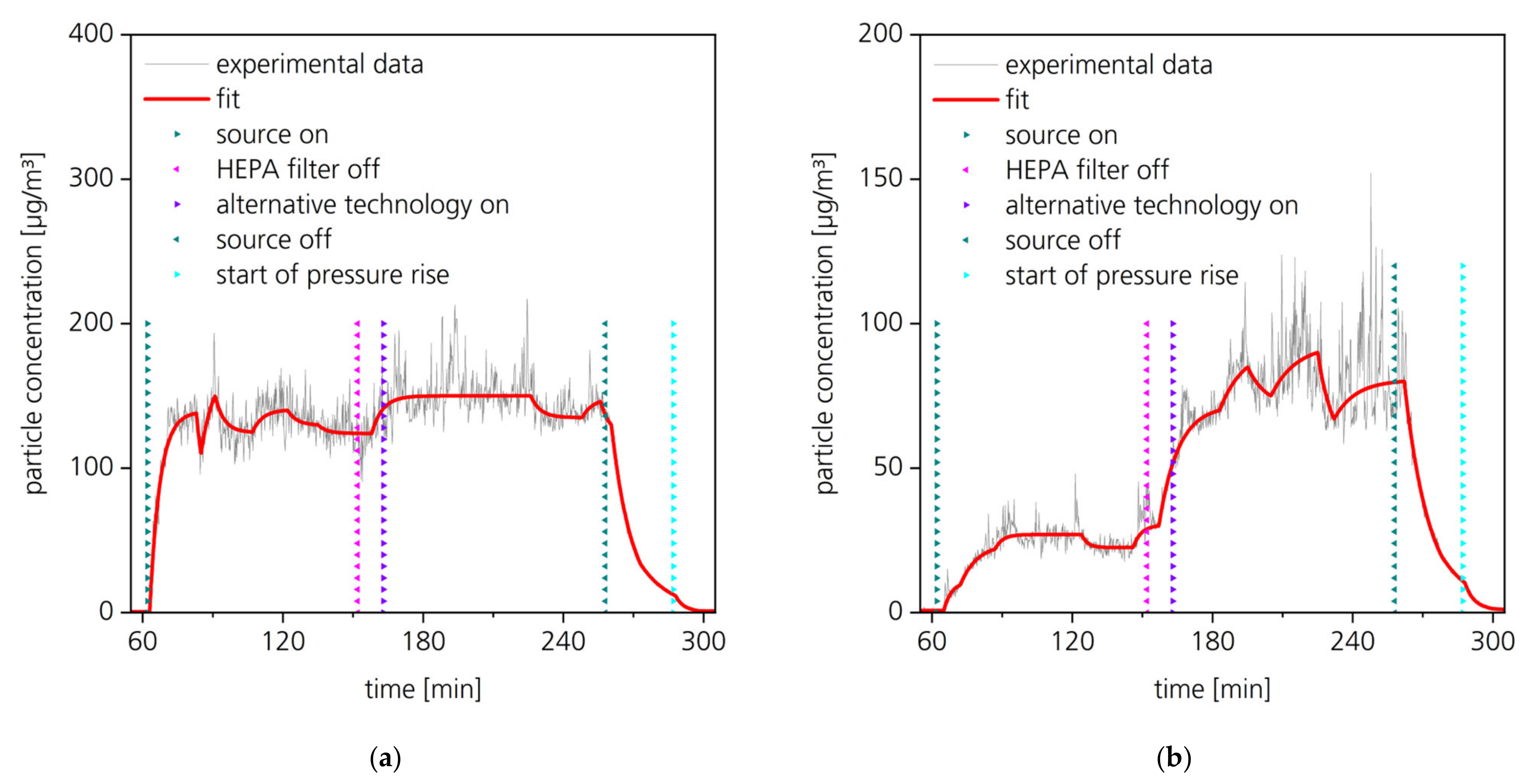
Figure 4a illustrates the fitting curve and the experimental data for the concentration at position 1 in the aircraft cabin close to the aerosol release. Figure 4b presents the trends of the parameters sn and kn at position 1, and the specific values can be extracted from Table 5. During the aerosol release, the total loss coefficient kn amounted to about 17 h−1 and the source term about 4420 (µg/m3)/h. When the aerosol release terminated, the loss coefficient kn initially increased for a short moment and afterward decreased in several steps from 28.3 down to 3.9 h−1. This result clearly indicates that the exponential decay coefficient is not constant over time. With the beginning of the pressure rise at 285 min, the coefficient kn increased again due to venting the cabin with fresh air.
At position 2 (Figure 5a) and especially at position 3 (Figure 5b), the particle concentration is smaller than at position 1 due to the larger distance from the aerosol source. While the change of the cleaning technique from HEPA filter to non-thermal plasma almost did not affect the concentration at position 1 and slightly at position 2, the concentration at position 3 increased by a factor of about 3. This is a clear indication that the purification effect of the cleaning technique depends on location in the aircraft cabin.
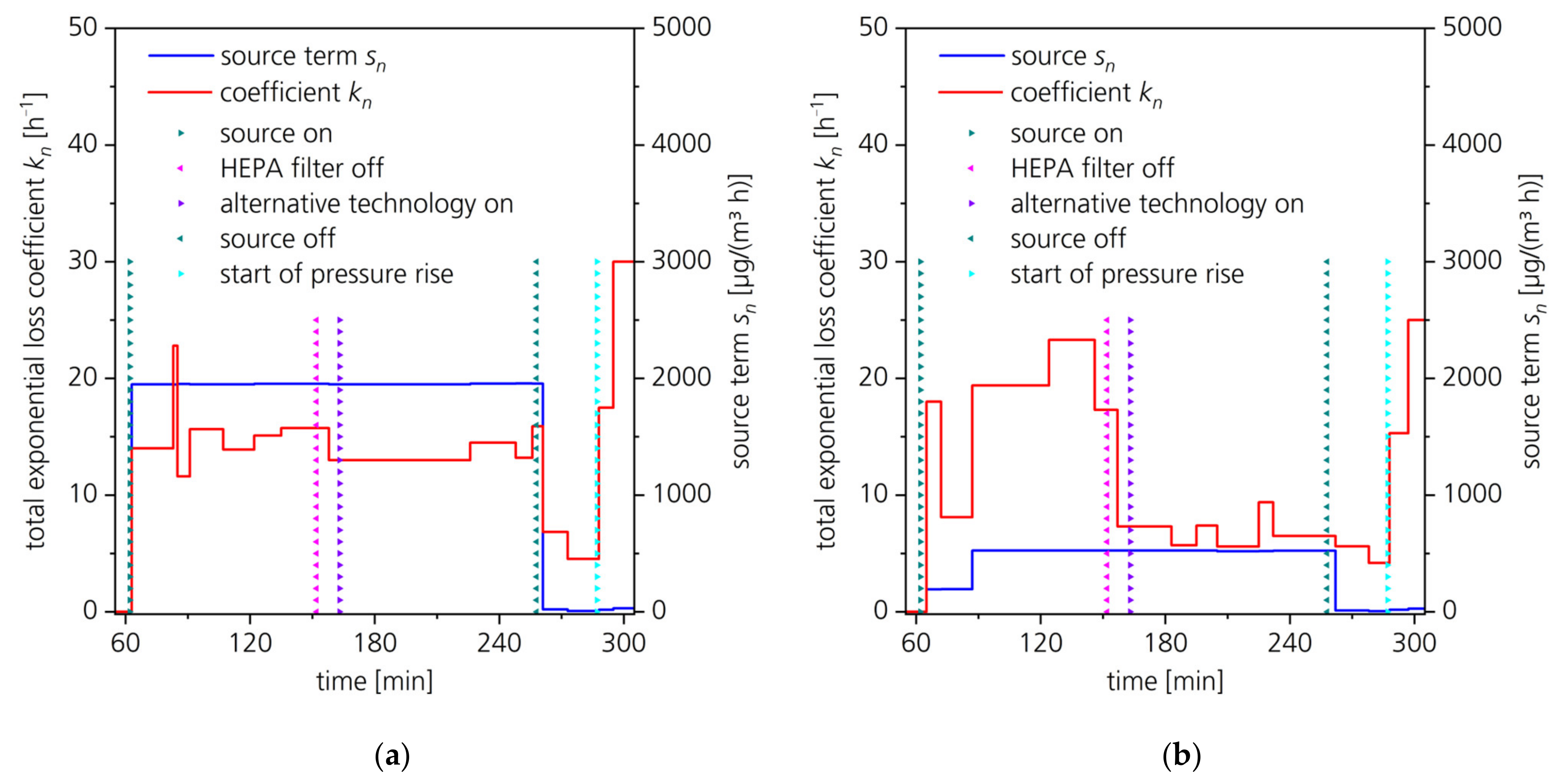
Figure 6 illustrates the trends of kn and sn at positions 2 and 3. Several changes of kn can be dedicated to events of the experimental schedule, like switching the aerosol release on and off, changing the cleaning technology, and the start of the pressure rise due to venting the aircraft cabin. The concentration drops and the increase of kn at positions 2 and 3 at about 123 min and 225 min (Table 6) correlated with the beginning of the air sampling for bacteriophage plaque assays. The volume flow of the sampling pumps was 3 m3/h and, therefore, in the range of typical respiratory flow volumes of approximately six passengers (0.5 m3/h per person). The reason for the lower source term sn during phases 1 and 2 at position 3 is unknown (194 instead of 524 (µg/m3)/h). Due to the low noise in phase 2, the variance of parameter k2 is low.

4. Discussion

4.1. Case Study I: Determination of a Clean Air Delivery Rate under Well Mixed Conditions

Usually, testing procedures for determining a CADR utilize an exponential decay without continuous particle release and hence without a source term [2,4,5,6,7]. Schumacher et al. presented an equation analogous to Equation (5). However, they did not utilize their model to analyze experimental data [3]. No CADR evaluation method considering an aerosol release during the testing period could be found in the literature besides the utilization of the presented model for the analysis of particulate matter and bacteriophage plaque assays by Burdack-Freitag et al. and Schmohl et al. [13,23].
With the presented test schedule in combination with the application of the presented incremental evaluation model, the clean air delivery rate could be determined accurately with about 5% of uncertainty. Additionally, this method is very robust because the fitting is done over a long period. Therefore, short-term artifacts do not influence the result (e.g., Figure 3, PM10 at 1.5 h). Furthermore, a continuous aerosol release is more realistic than tests without aerosol release during the testing of the air cleaner.
The particle size distribution of the used aerosol and the particle size dependency of the filter efficiency have to be considered to determine a CADR [2,3,6]. In this research, this aspect was neglected to reduce the complexity of the topic.
The purpose of case study I was to validate the incremental evaluation model under controlled experimental conditions and to demonstrate the excellent agreement of the mathematical model with the experimental data.

4.2. Case Study II: Investigation of an Air Cleaner in an Aircraft Cabin

Computer-assisted simulations are commonly used to compare experimental data with calculated data [28,29]. Numerical simulations can provide spatial and temporal resolved parameters in high resolution. However, the effort to create a numerical simulation model is much higher than the utilization of the presented incremental evaluation model.
Usually, the effectiveness of air purification is investigated by a test setup that reduces the complexity of the system. For instance, a single-pass collection effectiveness assessment can be used, and the concentration before and after the cleaning device can be compared [9]. However, due to this simplification, the influence of the distance neither to the particle source nor to the air inlets and outlets can be determined. Case study II provides the first experimentally derived spatial and temporal resolved source terms s and total loss coefficients k in an aircraft cabin, thus under complex flow conditions.
Jung utilized an equation similar to Equation (12) to describe the change of CO2 concentration in a car cabin [12]. However, no analysis with several time segments was executed.
The determined source terms in case study II were not equal to the release rate at Sheffield’s head because only a part of the released particles reached the volume compartment where the aerosol spectrometers measured the particle concentration. The further the position of the aerosol spectrometer from Sheffield’s head, the lower the source term. The realized source term in the volume compartment depends on flow characteristics. Therefore, a change in flow directions, for example, due to moving staff, can change the source term at a certain position. The assumption of a constant source term was used to reduce the complexity of the model. This can imply a shortcoming for the application of the incremental model. The set of parameters has to be plausible concerning the events and effects during the experiment.
Usual exponential decay models with a constant total loss coefficient were unsuitable for describing the concentration decay process after the aerosol release terminated. However, the presented incremental model could quantify the change of the total loss coefficient and the source term during the concentration decrease. At position 1, terminating the aerosol release resulted in a short increase of kn (up to 28.3 h−1) followed by a stabilization close to the kn (approx. 5 h−1) of positions 2 and 3. Physically, this indicates that the aerosol release in the proximity dominated and outperformed the benefit of the cleaning technology. Once the emission is terminated, the local particle cloud quickly dilutes until the concentration is homogeneous in the aircraft cabin (approx. 10 µg/m3 at 288 min). The results for all three positions indicate a slowdown of particle loss after the aerosol release terminated. Initially, the particle diffusion effect contributed to the particle loss resulting in a high total loss coefficient. Afterwards, the loss process was increasingly dominated by the air exchange. At all three positions, the following increase of particle loss at approx. 288 min correlated with the pressure rise while venting the cabin.
Compared with the mean air exchange of 7.9 h−1, the determined total loss coefficients were higher at all three positions (13–23 h−1) while the HEPA filter was used. With the non-thermal plasma cleaning technique, the total loss coefficient was in the same range at positions 1 and 2, but at position 3, the total loss coefficient dropped to approximately 7 h−1. The change of the total loss coefficient k during the experiment indicated whether the sampling position was affected mainly by the aerosol release or the air cleaning technology. The change of the cleaning technology resulted in a reduced total loss coefficient at position 3 (from 17.3 to 7.3 h−1). On the contrary, the change did not affect the total loss coefficient at position 1 (17.0 h−1 constantly). This interpretation is consistent with the higher source term s at position 1 (4420 (µg/m3)/h) in comparison with position 3 (approx. 520 (µg/m3)/h). These results confirmed the interpretation that the aerosol release in the proximity of the particle releasing source dominated and outperformed the benefit of the cleaning technology and that the particle diffusion effect contributed to the particle loss.
Additionally, the influence of a parallel air sampling for phage plaque assay could be quantified using the incremental model. The sampling resulted in an increase in the total loss coefficient at positions 2 (9–20%) and 3 (12–68%). An alternative set of parameters could be a stable loss coefficient combined with a reduced source term, but this option was assumed to be less plausible. The influence of parallel sampling should be considered in future investigations.

5. Conclusions and Outlook

5.1. Case Study I: Determination of a Clean Air Delivery Rate under Well Mixed Conditions

In realistic air cleaner applications, the source releases aerosol simultaneously while the air cleaner is purifying the indoor air without the support of external mixing, e.g., by fans. Air cleaners should be tested under similar conditions. Therefore, the testing procedure described in Table 7 is recommended for evaluating air cleaners.
With the suggested testing procedure, it can be proved that the air cleaner can mix the air in the test room independently of the external air mixing devices during phases 4 and 5 (fan off). Subsequently, the last two phases can be applied to prove the stability of the aerosol generation (step 6, in combination with knat from step 7) and the natural loss coefficient knat (step 7).
In phases 4 and 5, the well-mixed condition is potentially not fulfilled. For these two phases, the data can be evaluated by the incremental model analogous to the scenario in the aircraft cabin (case study II).

5.2. Case Study II: Investigation of an Air Cleaner in an Aircraft Cabin

Spatial and temporal resolved source terms s and total loss coefficients k could be derived from the available experimental data. Thus, the local effectiveness of the air cleaning technology could be evaluated more reliably than without the application of the incremental evaluation model. Likewise, identifying some disturbance factors was possible (e.g., the effect of parallel air sampling on the total loss coefficient k or change of the source term s at position 3 at 87 min).

5.3. Applications beyond the Presented Case Studies

The presented model is limited to scenarios with zero-order and first-order kinetics processes. An adaptation of the equation is potentially needed if processes with second-order kinetics, such as chemical reactions of two air components, have to be considered. The effects independent of the concentration (=zero-order kinetics) affect the source term s, and the effects with first-order kinetics concerning the concentration affect the total loss coefficient k. The individual effects contributing to the source term s and the total loss coefficient k have to be determined by a suitable design of the experiment, such as changing between periods with and without the purifying technology (or source, respectively). Additionally, the model could be extended with a release rate as a function of time.
With the incremental fitting model, even complex and challenging experiments with dynamic conditions can be described. The practical benefits are:
-
Spatial and temporal resolved quantification of source terms s and total loss coefficients k;
-
More reliable evaluation of the local effectiveness of an air purifying technology;
-
Support in the identification of disturbance factors;
-
Determination of the spatial and temporal resolved air exchange rate in indoor spaces, e.g., by a parallel controlled release of CO2;
-
Assistance in the planning of experiments through the prediction of expected matter concentrations and necessary sampling volumes (analogous to Schumacher et al. [3]).
Usually, the incremental evaluation model can be used independently from the kind of matter. For example, concentration curves of volatile organic compounds (VOC), CO2 [12], N2O [15], NO2, NO, and Ozone [13] can also be analyzed. For instance, Jung utilized an equation analogous to Equation (12) to determine the evolution of the CO2 concentration in car cabins, but without changing the experimental conditions and hence not as an incremental model [12]. Furthermore, the analysis of bioaerosols using plaque assays is feasible [13,23]. In the case of using air samples, such as for bacteriophage plaque assays, the integral of Equation (12) is needed [23]. Further investigations to evaluate the robustness of this tool are necessary and should proceed in future research. An objective and future topic is the transfer of the equations into a comfortably manageable evaluation tool.

Author Contributions

Conceptualization, A.S.; methodology, A.S., V.N. and M.B.; software, A.S.; validation, A.S., M.B. and V.N.; formal analysis, A.S.; investigation, M.B. and V.N.; resources, V.N. and M.B.; data curation, A.S. and M.B.; writing—original draft preparation, A.S. and M.B.; writing—review and editing, A.S., M.B., V.N., C.R.S., P.A.V.G. and C.S.; visualization, A.S. and M.B.; supervision, V.N. and S.J.; project administration, V.N. and S.J.; funding acquisition, V.N. and A.B.-F. All authors have read and agreed to the published version of the manuscript.

Funding

This research was funded by the Bavarian Ministry of Economic Affairs, Regional Development and Energy, aviation research program BayLu25, grant number ROB-2-3410.20_04-10-33/BLU-2109-0033.

Institutional Review Board Statement

Not applicable.

Informed Consent Statement

Not applicable.

Data Availability Statement

The data set is available from the corresponding author upon reasonable request.

Conflicts of Interest

The authors declare no conflict of interest. The funders had no role in the design of the study, in the collection, analyses, or interpretation of data, in the writing of the manuscript, or in the decision to publish the results.

References

  1. Curtius, J.; Granzin, M.; Schrod, J. Testing mobile air purifiers in a school classroom: Reducing the airborne transmission risk for SARS-CoV-2. Aerosol Sci. Technol. 2021, 55, 586–599. [Google Scholar] [CrossRef]
  2. Küpper, M.; Asbach, C.; Schneiderwind, U.; Finger, H.; Spiegelhoff, D.; Schumacher, S. Testing of an Indoor Air Cleaner for Particulate Pollutants under Realistic Conditions in an Office Room. Aerosol Air Qual. Res. 2019, 19, 1655–1665. [Google Scholar] [CrossRef] [Green Version]
  3. Schumacher, S.; Asbach, C.; Schmid, H.-J. Effektivität von Luftreinigern zur Reduzierung des COVID-19-Infektionsrisikos/Efficacy of air purifiers in reducing the risk of COVID-19 infections. Gefahrstoffe 2021, 81, 16–28. [Google Scholar] [CrossRef]
  4. ANSI/AHAM AC-1-2020; Method for Measuring Performance of Portable Household Electric Room Air Cleaners. Association of Home Appliance Manufacturers: Washington, DC, USA, 2020.
  5. GB/T 18801-2015; Air Cleaner (Translated English version of Chinese National Standard). National Standard of the People’s Republic of China: Beijing, China, 2016.
  6. Wood, J. Evaluation of In-Room Particulate Matter Air Filtration Devices; EPA/600/R-08/012; Environmental Protection Agency: Washington, DC, USA, 2008; pp. 1–56.
  7. VDI-EE 4300 Blatt 14:2021-09; Measurement of Indoor Pollution—Requirements for Mobile Air Purifiers to Reduce Aerosol-Borne Transmission of Infectious Diseases. Verein Deutscher Ingenieure e.V.: Düsseldorf, Germany, 2021.
  8. Mølgaard, B.; Koivisto, A.J.; Hussein, T.; Hämeri, K. A New Clean Air Delivery Rate Test Applied to Five Portable Indoor Air Cleaners. Aerosol Sci. Technol. 2014, 48, 409–417. [Google Scholar] [CrossRef]
  9. Pellegrin, B.; Berne, P.; Giraud, H.; Roussey, A. Exploring the potential of electrostatic precipitation as an alternative particulate matter filtration system in aircraft cabins. Indoor Air 2022, 32, e12990. [Google Scholar] [CrossRef] [PubMed]
  10. Reed, C.; Nabinger, S.J.; Emmerich, S.J. Measurement and simulation of the indoor air quality impact of gaseous air cleaners in a test house. Proc. Indoor Air 2002, 2, 652–657. [Google Scholar]
  11. Chan, W.R.; Logue, J.M.; Wu, X.; Klepeis, N.E.; Fisk, W.J.; Noris, F.; Singer, B.C. Quantifying fine particle emission events from time-resolved measurements: Method description and application to 18 California low-income apartments. Indoor Air 2018, 28, 89–101. [Google Scholar] [CrossRef] [PubMed] [Green Version]
  12. Jung, H. Modeling CO2 Concentrations in Vehicle Cabin; SAE Technical Paper 2013-01-1497; SAE International: Warrendale, PA, USA, 2013; pp. 1–6. [Google Scholar] [CrossRef]
  13. Burdack-Freitag, A.; Buschhaus, M.; Grün, G.; Hofbauer, W.K.; Johann, S.; Nagele-Renzl, A.M.; Schmohl, A.; Scherer, C.R. Particulate Matter versus Airborne Viruses—Distinctive Differences between Filtering and Inactivating Air Cleaning Technologies. Atmosphere 2022, 13, 1575. [Google Scholar] [CrossRef]
  14. Manoukian, A.; Quivet, E.; Temime-Roussel, B.; Nicolas, M.; Maupetit, F.; Wortham, H. Emission characteristics of air pollutants from incense and candle burning in indoor atmospheres. Environ. Sci. Pollut. Res. 2013, 20, 4659–4670. [Google Scholar] [CrossRef]
  15. Bivolarova, M.; Ondráček, J.; Melikov, A.; Ždímal, V. A comparison between tracer gas and aerosol particles distribution indoors: The impact of ventilation rate, interaction of airflows, and presence of objects. Indoor Air 2017, 27, 1201–1212. [Google Scholar] [CrossRef] [PubMed]
  16. Nazaroff, W.W.; Cass, G.R. Mathematical modeling of indoor aerosol dynamics. Environ. Sci. Technol. 1989, 23, 157–166. [Google Scholar] [CrossRef]
  17. Nazaroff, W.W. Indoor particle dynamics. Indoor Air 2004, 14, 175–183. Available online: https://escholarship.org/uc/item/7sq4x34d (accessed on 29 August 2022). [CrossRef] [PubMed] [Green Version]
  18. Nazaroff, W.W. Indoor bioaerosol dynamics. Indoor Air 2016, 26, 61–78. [Google Scholar] [CrossRef] [PubMed] [Green Version]
  19. Silcott, D.; Kinahan, S.; Santarpia, J. TRANSCOM/AMC Commercial Aircraft Cabin Aerosol Dispersion Tests. 2020. Available online: https://www.ustranscom.mil/cmd/docs/TRANSCOM%20Report%20Final.pdf (accessed on 29 August 2022).
  20. Zee, M.; Davis, A.C.; Clark, A.D.; Wu, T.; Jones, S.P.; Waite, L.L.; Cummins, J.J.; Olson, N.A. Computational fluid dynamics modeling of cough transport in an aircraft cabin. Sci. Rep. 2021, 11, 23329. [Google Scholar] [CrossRef] [PubMed]
  21. Matheis, C.; Norrefeldt, V.; Will, H.; Herrmann, T.; Noethlichs, B.; Eckhardt, M.; Stiebritz, A.; Jansson, M.; Schön, M. Modeling the Airborne Transmission of SARS-CoV-2 in Public Transport. Atmosphere 2022, 13, 389. [Google Scholar] [CrossRef]
  22. Woodward, H.; Fan, S.; Bhagat, R.K.; Dadonau, M.; Wykes, M.D.; Martin, E.; Hama, S.; Tiwari, A.; Dalziel, S.B.; Jones, R.L.; et al. Air Flow Experiments on a Train Carriage—Towards Understanding the Risk of Airborne Transmission. Atmosphere 2021, 12, 1267. [Google Scholar] [CrossRef]
  23. Schmohl, A.; Nagele-Renzl, A.M.; Buschhaus, M.; Johann, S.; Scherer, C.R.; Grün, G.; Hofbauer, W.K.; Burdack-Freitag, A. Determination of CADR of virus-inactivating air purifiers by surrogate virus plaque assay. In Proceedings of the Indoor Air 2022, 17th International Conference of the International Society of Indoor Air Quality & Climate, Kuopio, Finland, 12–16 June 2022; pp. 1–8. [Google Scholar]
  24. AHAM AC-5-2022; Method for Assessing the Reduction Rate of Key Bioaerosols by Portable Air Cleaners Using an Aerobiology Test Chamber. Association of Home Appliance Manufacturers: Washington, DC, USA, 2022.
  25. Baer, A.; Kehn-Hall, K. Viral concentration determination through plaque assays: Using traditional and novel overlay systems. J. Vis. Exp. 2014, 93, e52065. [Google Scholar] [CrossRef] [PubMed]
  26. DIN EN 13610:2003-06; Chemische Desinfektionsmittel—Quantitativer Suspensionsversuch zur Bestimmung der Viruziden Wirkung Gegenüber Bakteriophagen von Chemischen Desinfektionsmitteln in den Bereichen Lebensmittel und Industrie—Prüfverfahren und Anforderungen (Phase 2, Stufe 1). Deutsche Fassung EN 13610:2003; Deutsches Institut für Normung e.V.: Berlin, Germany, 2003.
  27. Norrefeldt, V.; Buschhaus, M.; Nagele-Renzl, A.M. European Patent Application: Aerosolgenerator und Verfahren zur Abgabe eines Aerosols. Patent Application No. 21212872.2, 7 December 2021. [Google Scholar]
  28. Dbouk, T.; Roger, F.; Drikakis, D. Reducing indoor virus transmission using air purifiers. Phys. Fluids 2021, 33, 103301. [Google Scholar] [CrossRef] [PubMed]
  29. Burgmann, S.; Janoske, U. Transmission and reduction of aerosols in classrooms using air purifier systems. Phys. Fluids 2021, 33, 033321. [Google Scholar] [CrossRef] [PubMed]
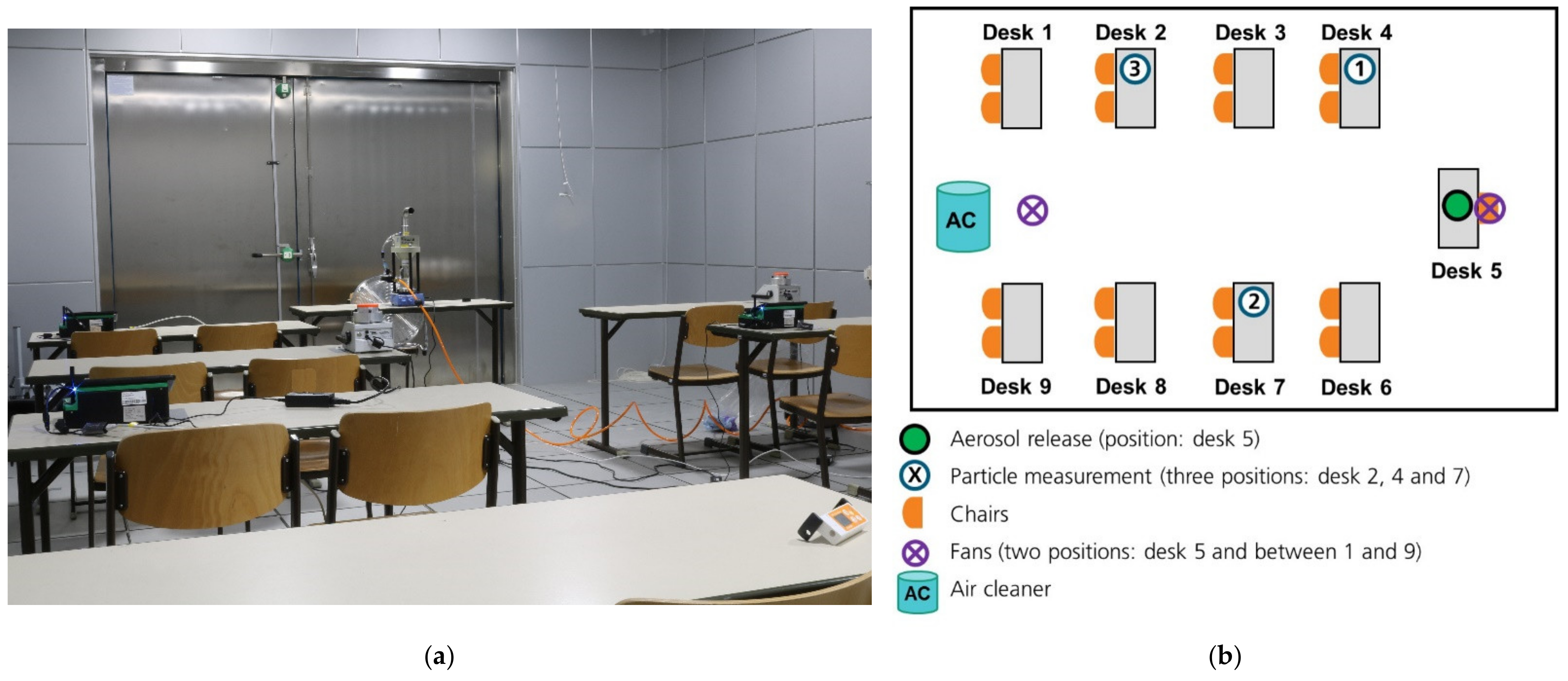
Figure 1. IATC test setup with one aerosol generator, two fans, one air cleaner, and three particle measurement devices: (a) view towards aerosol generator; (b) positions of the aerosol generator, three particle counters, and the air cleaner (AC) in the test room.
Atmosphere 13 01655 g001
Figure 2. Aircraft cabin and positions: (a) interior view; (b) positions of the Sheffield head, three particle counters, two air samplers for phage plaque assay, and 25 heated dummies.
Atmosphere 13 01655 g002
Figure 3. Determination of the coefficient kAC of an air cleaner (AC) in a well-mixed room. The natural loss coefficient is determined between 0 and 1 h. (Fitting process see Section 3.1.2.).
Atmosphere 13 01655 g003
Figure 4. Results of the particle measurement and fitting process at position 1 close to the aerosol release and the changed parameters like source on/off, start of pressure rise, and change of air cleaning technique and: (a) PM2.5 and corresponding fitting curve; (b) parameters kn and sn of the fitting curve.
Atmosphere 13 01655 g004
Figure 5. Experimental data of particle measurement (grey line) and fitted curve (red line) at positions in farther distance to the particle release: (a) PM2.5 at position 2; (b) PM2.5 at position 3.
Atmosphere 13 01655 g005
Figure 6. Fitted parameters kn and sn and changed parameters like source on/off, start of pressure rise, and change of air cleaning technique: (a) kn and sn at position 2; (b) kn and sn at position 3.
Atmosphere 13 01655 g006
Table 1. Events during determining the clean air delivery rate of an air cleaner in a well-mixed test room.
Time of Daytevent
[h]
Event
11:30−0.50Start of particle measurement
12:000.00Aerosol release was switched on.
13:001.00Air cleaner with 100% power level was switched on.
14:002.00Aerosol release was switched off.
14:402.67Aerosol release was switched on and air cleaner reduced from 100% to 50% power level.
15:403.67Aerosol release was switched off.
17:005.00End of particle measurement
Table 2. Documented events during the investigation in the aircraft cabin.
Time of Daytevent
[min]
Event
08:00−30Ventilation with HEPA filter switched on
08:388Start of particle measurement
09:1747Takeoff (pressure drop from 946 hPa to 750 hPa)
09:3161Cruising altitude reached (750 hPa)
09:3262Start of aerosol release (Sheffield head close to position 1)
10:30120Start of phage sampling
11:00150End of phage sampling
11:02152HEPA filter removed
11:13163Alternative technology on
12:13223Start of phage sampling
12:43253End of phage sampling
12:48258End of aerosol release
13:17287Descent (pressure rise from 750 hPa to 946 hPa)
13:21291Alternative technology off
13:34304Landing (946 hPa)
13:35305End of particle measurement
Table 3. Resulting set of equations for the five segments of the incremental model.
Phase
n *
Start tn−1End tn f n t   with   N = k n a t / 1 exp k n a t × t 1 t 0
ntn−1tn f n t = N × r n / k n + f n 1 N × r n / k n × exp k n × t t n 1 with k n = k n a t + p n × e n × k A C
101.00 f 1 t = N × 1 / k 1 + 0 N × 1 / k 1 × exp k 1 × t 0 with k 1 = k n a t + 0 × 0 × k A C
21.002.00 f 2 t = N × 1 / k 2 + 1 N × 1 / k 2 × exp k 2 × t 1.00 with k 2 = k n a t + 1 × 1 × k A C
32.002.67 f 3 t = N × 0 / k 3 + f 2 t 2 N × 0 / k 3 × exp k 3 × t 2.00 with k 3 = k n a t + 1 × 1 × k A C
42.673.67 f 4 t = N × 1 / k 4 + f 3 t 3 N × 1 / k 4 × exp k 4 × t 2.67 with k 4 = k n a t + 0.5 × e 50 % × k A C
53.675.00 f 5 t = N × 0 / k 5 + f 4 t 4 N × 0 / k 5 × exp k 5 × t 3.67 with k 5 = k n a t + 0.5 × e 50 % × k A C
* The fitted curve was divided in five segments with known or defined parameters tn−1, f0, f1, rn, pn, e0% = 0, e100% = 1 and three unknown variables knat, kAC and e50%.
Table 4. Known parameters tn−1, pn, and r, and variable fitting parameters knat, kAC, and e50% for the fitting curve in Figure 3.
Phase n *
[-]
tn−1 (Start)
[h]
knat
[h−1]
kAC
[h−1]
AC
Power Level p
AC
Efficiency e
Release
r
kn
[h−1]
fstart,n
[-]
feq,n
[-]
10.000.53.00% (off)-1 (on)0.50.002.51
21.020.53.0100% (on)e100% = 11 (on)3.51.000.36
32.020.53.0100% (on)e100% = 10 (off)3.50.380.00
42.680.53.050% (on)e50% = 1.141 (on)2.210.040.57
53.680.53.050% (on)e50% = 1.140 (off)2.210.520.00
* The fitted curve was divided into five model segments with individual parameters p, e, and r. The fitting parameters knat and kAC have been kept constant for all five segments. Bold type numbers are unknown variables used for matching the curve to the measurement data.
Table 5. Fitting parameters kn and sn for the fitting curve for position 1 and derived concentration cstart,n at the beginning of phase n and equilibrium concentration ceq,n.
Position
in Cabin
Phase n *
[-]
tn (Start) #
[min]
kn
[h−1]
Uncertainty Factor of knsn
[(µg/m3)/h]
Uncertainty Factor of sncstart,n
[µg/m3]
ceq,n
[µg/m3]
Position
1
163.517.01.444201.41.0260
2259.728.31.14352.02609.2
3260.915.81.05942.01483.5
42629.31.05232.01112.4
52666.71.05112.060.01.6
62705.31.0572.038.81.3
72745.11.0551.927.51.0
82833.91.0541.713.41.0
928915.71.05141.29.41.0
1029430.01.0521.23.40.4
* The fitted curve was divided into ten phases with individual fitting parameters kn and sn in each phase n. # The aerosol was generated between 62 min and 258 min while the pressure continuously was 750 hPa. Between 120 min and 150 min, as well as between 223 min and 253 min, microbiological sampling with 3 m3/h proceeded. At 150 min, the HEPA filter was removed, and at 163 min, the alternative cleaning technology was built in. Venting the cabin started at 285 min.
Table 6. Fitting parameters kn and sn for the fitting curves for position 2 and position 3 and derived concentrations cstart,n at the beginning of phase n and equilibrium concentrations ceq,n. The bold type values were used for the initial determination of kn. In the other phases, the assumption of a constant source term was applicated.
Position
in Cabin
Phase n *
[-]
tn (Start) #
[min]
kn
[h−1]
Uncertainty Factor of knsn
[(µg/m3)/h)]
Uncertainty Factor of sncstart,n
[µg/m3]
ceq,n
[µg/m3]
Position
2
16314.01.519501.50.5139
28322.82.019472.913885.4
38511.62.019521.8110168
49115.652.019502.0150125
510713.92.019502.0125140
612215.12.019532.0140129
713515.752.019532.0130124
815813.02.019502.0124150
922614.52.019562.0150135
1024813.22.019572.0135148
1125615.92.019562.2146123
122616.841.1212.01303.1
132734.531.162.0321.3
1428817.51.1171.4111.0
1529530.01.1301.02.31.0
Position
3
16518.02.01931.70.710.7
2728.11.41941.39.523.9
38719.42.05242.022.027.0
412423.32.05242.027.022.5
514617.32.05251.922.530.3
61577.31.45241.430.071.8
71835.72.05251.870.092.1
81957.42.05252.285.070.9
92055.62.05191.875.0101.1
102259.42.05212.494.061.1
112326.52.05232.067.080.5
122625.611.1122.081.02.1
132784.191.152.019.01.1
1428815.31.1171.210.01.1
1529725.01.1271.02.01.1
* Each fitted curve was divided into 15 phases with individual fitting parameters kn and sn in each phase n. # The aerosol was generated between 62 min and 258 min while the pressure was continuously 750 hPa. Between 120 min and 150 min, as well as between 223 min and 253 min, microbiological sampling with 3 m3/h proceeded. At 150 min, the HEPA filter was removed, and at 163 min the alternative cleaning technology was built in. Venting the cabin started at 285 min.
Table 7. Recommended testing procedure for the evaluation of air cleaners.
Phase
n
tstart
[h]
Aerosol
Release
Air
Cleaner
Both
Fans
Purpose
10.0onoffondetermination of knat,start under ideal, well-mixed conditions
21.00ononon2 & 3: determination of kAC,ideal under ideal, well-mixed conditions
31.67offonon
42.33ononoff4 & 5: determination of kAC,real under realistic conditions
53.00offonoff
63.67onoffonproof of stable aerosol generation by comparison with phase 1
74.33 *offoffonproof of stable knat by comparison of knat,end (n = 7) with knat,start (n = 1)
* End of phase 7 at 5.00 h.
Publisher’s Note: MDPI stays neutral with regard to jurisdictional claims in published maps and institutional affiliations.