1. Introduction
Since the 1990s, a new discipline, space weather, has been developing. One of its definitions is that: “Space weather is the physical and phenomenological state of natural space environments. The associated discipline aims, through observation, monitoring, analysis and modeling, at understanding and predicting the state of the Sun, the interplanetary and planetary environments, and the solar and non-solar driven perturbations that affect them; and also at forecasting and now casting the possible impacts on biological and technological systems [
1]”. Space weather must integrate all knowledge concerning Sun–Earth relations and predict the impact of solar events on new technologies and biological systems.
For several decades, many scientific disciplines relating to Sun–Earth relations (solar physics, internal and external geophysics, atmospheric physics, etc.) have developed separately. Space weather requires breaking down the boundaries that separate these disciplines. Certain physical processes are common to these different scientific disciplines such as the dynamo process. The process of the dynamo connects together through the formalism of Maxwell, so many physical parameters (movement of the plasma, magnetic field, electric currents, etc.) and the magnetic field are easily measurable.
We therefore propose to group together different disciplines using the dynamo process in this article. Before this study, the dynamo mechanism was/is invoked for the Sun [
2], for the magnetosphere [
3], for the ionosphere [
4], and for the Earth [
5]. Our novelty will be to develop a transdisciplinary approach of the Earth–Sun system to aid in the analysis of the Earth’s magnetic field at mid- and low-latitudes. In the
Section 2, we briefly recall the four permanent large-scale dynamos of the Earth–Sun System. In the
Section 3, we present the magnetic signatures of some large-scale electric current systems circulating in the ionosphere and magnetosphere. Then, in
Section 3, we discuss the variations in the Earth’s magnetic field, and explain how to treat the magnetic signatures of electric currents in middle and low latitudes in order to extract the magnetic effect of the ionospheric disturbance dynamo [
6,
7,
8].
2. Dynamos in the Earth–Sun System: Physics
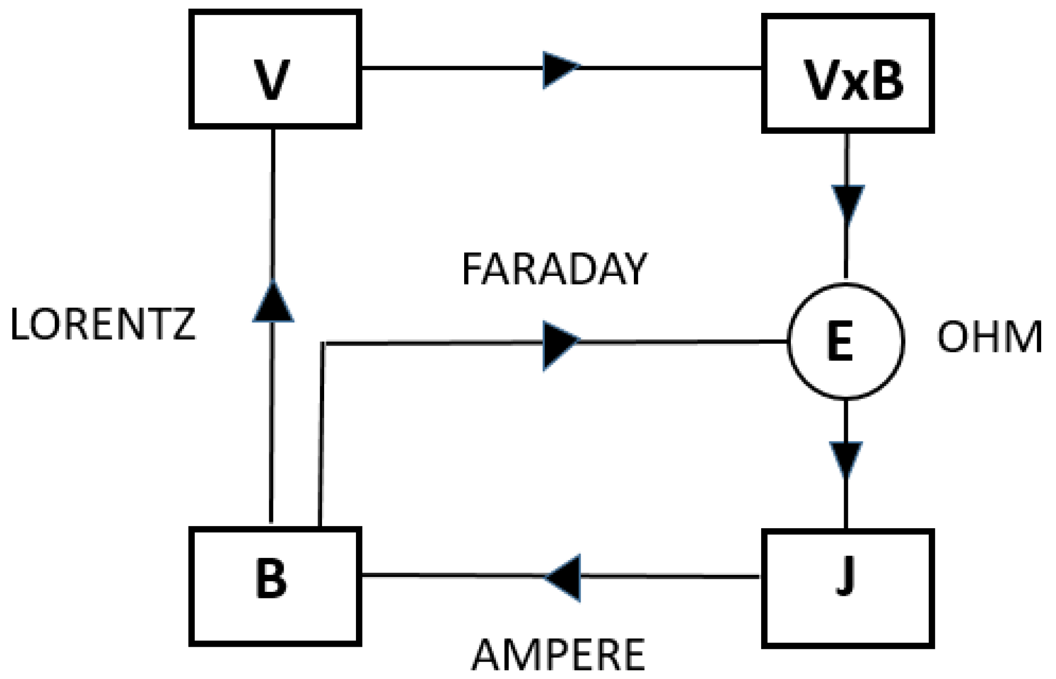
A motion V and a magnetic field B are the two creative elements of a dynamo.
Figure 1 presents the dynamo physics. A dynamo converts kinetic energy into electric-magnetic energy. “
A motion V across a magnetic field B induces an electric field V ×
B, which produces an electric current J = σ (E + V ×
B) via
Ohm’s law where σ is the electric conductivity and E an electric field. This current produces in turn a magnetic field ∇XB = μJ, where μ is the permeability. The magnetic field creates both electric field E through Faraday’s law ε = −∂Φ
B/∂t
and Lorentz force J × B which reacts on the motion V” [
2].
The dynamo theory describes the process by which rotation with convective motion in a conductive fluid acts to maintain a magnetic field. This theory explains the presence of long-term magnetic fields in astronomical bodies. The dynamo effect is also called the etohydrodynamics (MHD) mechanism, which was originally proposed to explain the origin of elds observed in galaxies and galaxy clusters. The basic physics idea is to convert the kinetic energy of turbulent motion in the interstellar medium into magnetic energy. Initiating the galactic MHD process requires a seed magnetic field as well as three other key components: hydrodynamic turbulence, differential rotation, and the rapid reconnection of magnetic field lines. Due to the magnetohydrodynamics effect, a strong magnetic field of magnitude 10
12–10
15 T can be generated inside a newly-formed hot neutron star [
9,
10]. If both toroidal and poloidal magnetic fields exist inside a neutron star, the star’s structure tends to be stable. The dissipation of poloidal magnetic fields provides photon and neutrino radiation from the stellar surface, while the decay of the dipolar poloidal magnetic fields affects the rotation evolution of the star [
11,
12].
2.1. The Solar Dynamo (Solar Physics)
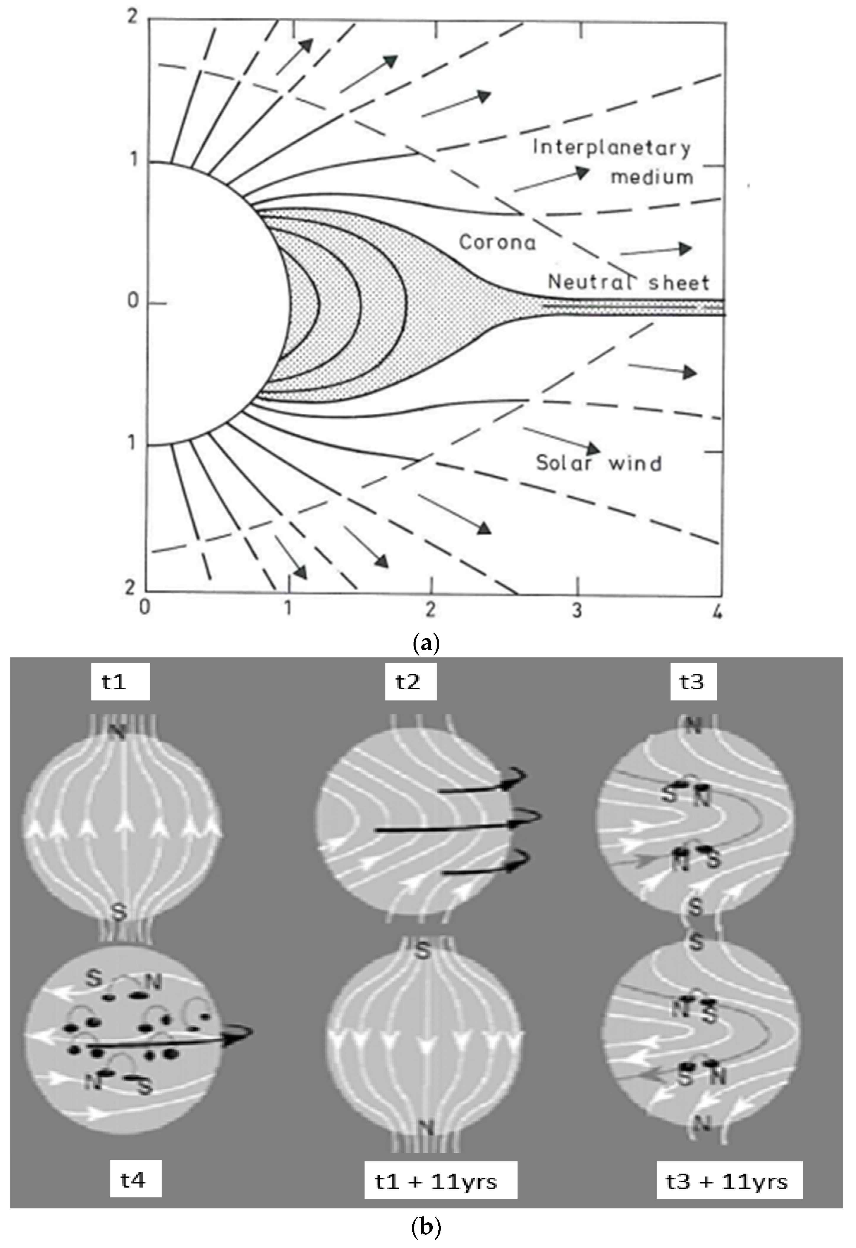
The solar magnetic field is highly variable, which makes the solar wind and the magnetic field it carries with it into interplanetary space highly variable in space and in time. In a first approximation, the magnetic field near the visible solar surface can be regarded as a dipole similar to that of the Earth. The solar magnetic field is shown in
Figure 2a [
13], it reverses every eleven years, and its magnitude is 5 × 10
−3 T. The Sun also rotates on itself, with a period of approximately 27 Earth days. It rotates faster at the equator (25 days) than at the poles (35 days). The lines of the dipole field are twisted under the effect of the differential rotation and this creates the sunspots whose magnetic force is 0.3 to 0.5 T.
Figure 2b [
7] represents the complete solar cycle with dipole phases alternating with toroidal phases (
http://solarscience.msf.nasa.gov/dynamo.shtml (accessed on 13 October 2022) for more details on the solar dynamo).
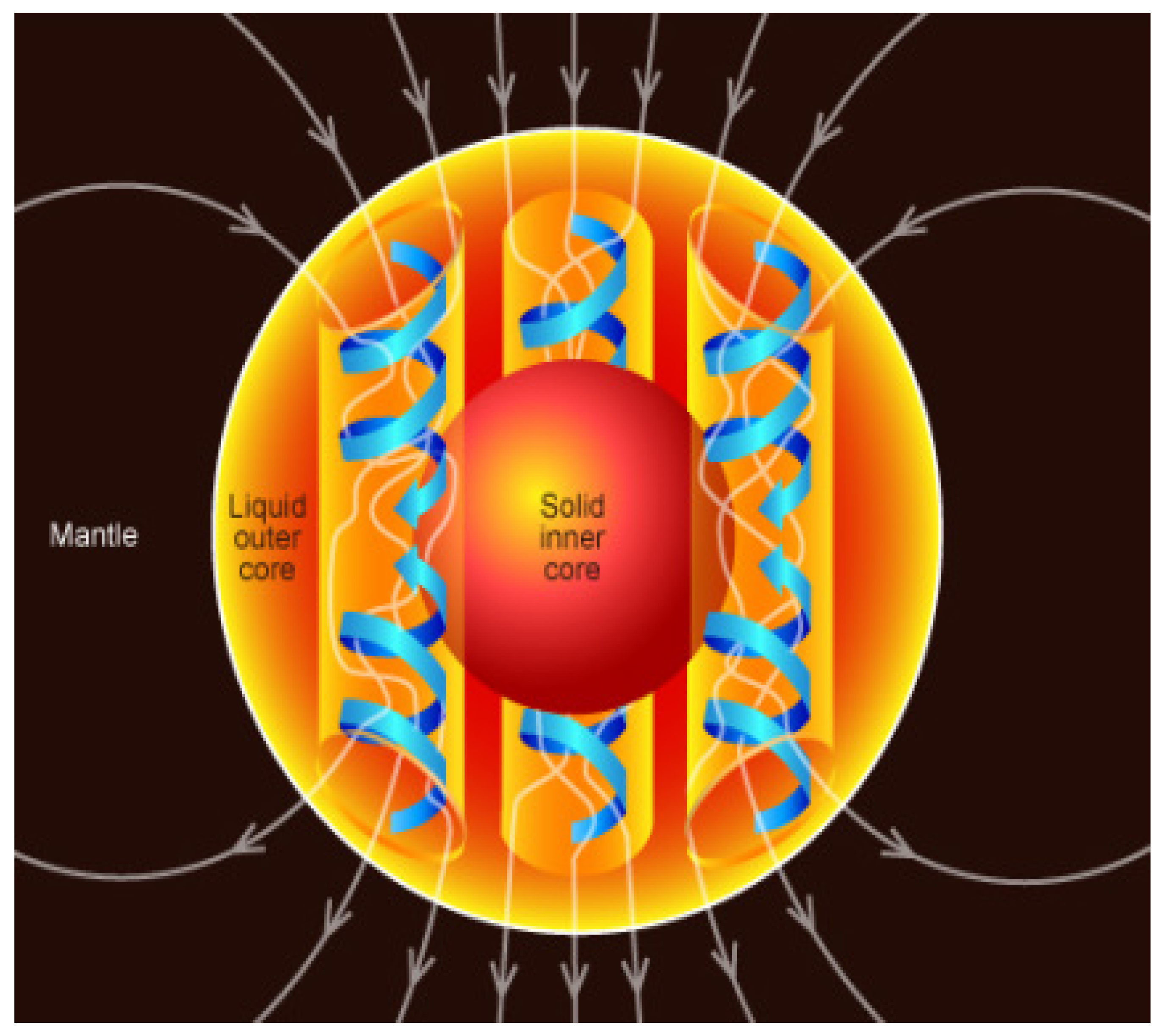
2.2. The Terrestrial Dynamo (Internal Geophysics)
The dynamo effect at the origin of the Earth’s magnetic field is reduced by the induction generated by the rapid movements of the alloys of iron and nickel in fusion in the liquid part [
5]. In the first approximation, the Earth’s magnetic field is a magnetic dipole. The community of geophysicists has developed a model of the terrestrial magnetic field IGRF,
https://www.ngdc.noaa.gov/IAGA/vmod/igrf.html (accessed on 13 October 2022).
Figure 3 illustrates the magnetic field [
15].
2.3. Connections between the Sun and the Earth
The Sun and the Earth are two magnetic bodies in motion. The Sun interacts with the Earth through different channels. The two main channels are electromagnetic emissions and solar wind.
Electromagnetic emissions from the sun range from short wave radiation to long wave radiations (from gamma rays, X rays, UV … to radio waves)
The solar wind is the constant stream of solar coronal material that flows off the Sun. It consists mostly of electrons, protons, and alpha particles, with energies usually between 1.5 and 10 keV. The solar wind transports a part of the solar magnetic field (IMF, interplanetary magnetic field). These two main channels of communication between the Sun and the Earth produce a dynamo effect in the Earth’s environment.
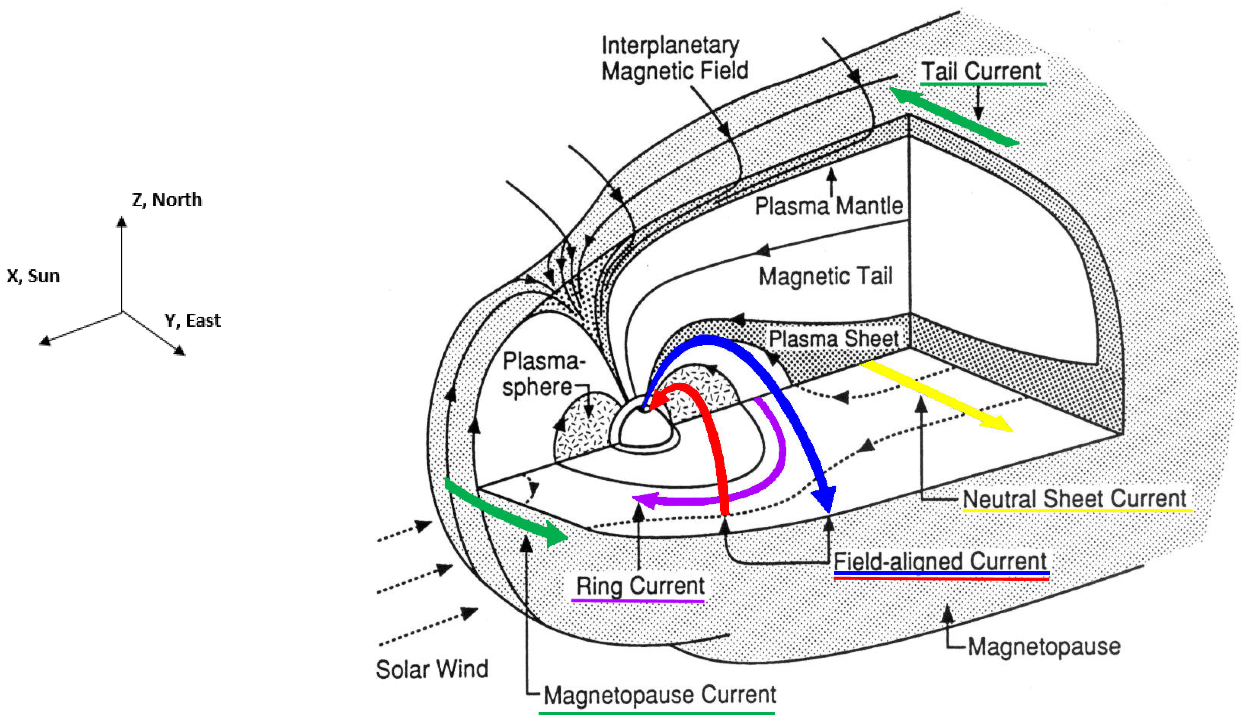
2.4. The Solar Wind Magnetosphere Dynamo (Solar Wind and Magnetosphere Physics)
The solar wind is a moving magnetized plasma, which interacts with the Earth’s magnetic field. The solar wind transfers energy to the magnetosphere [
16]. Two physical processes allow this transfer: (1) the viscous interaction between the solar wind and the magnetosphere [
17] and (2) the magnetic reconnection [
18]. Electric currents are associated with this dynamo. This is illustrated in
Figure 4. There are (1) the magnetopause electric current (Chapman Ferraro currents) circulating on the nose of the magnetosphere [
19]; (2) the ring current circulating in the equatorial plane of the magnetosphere at a distance of several radius of the Earth [
20]; (3) neutral sheet current; and (4) the tail current [
21]. All of these electric currents have a clear magnetic signature on the Earth’s magnetic field at the ground level, except for the field aligned current (Birkeland current) connecting the magnetosphere to the ionosphere [
22].
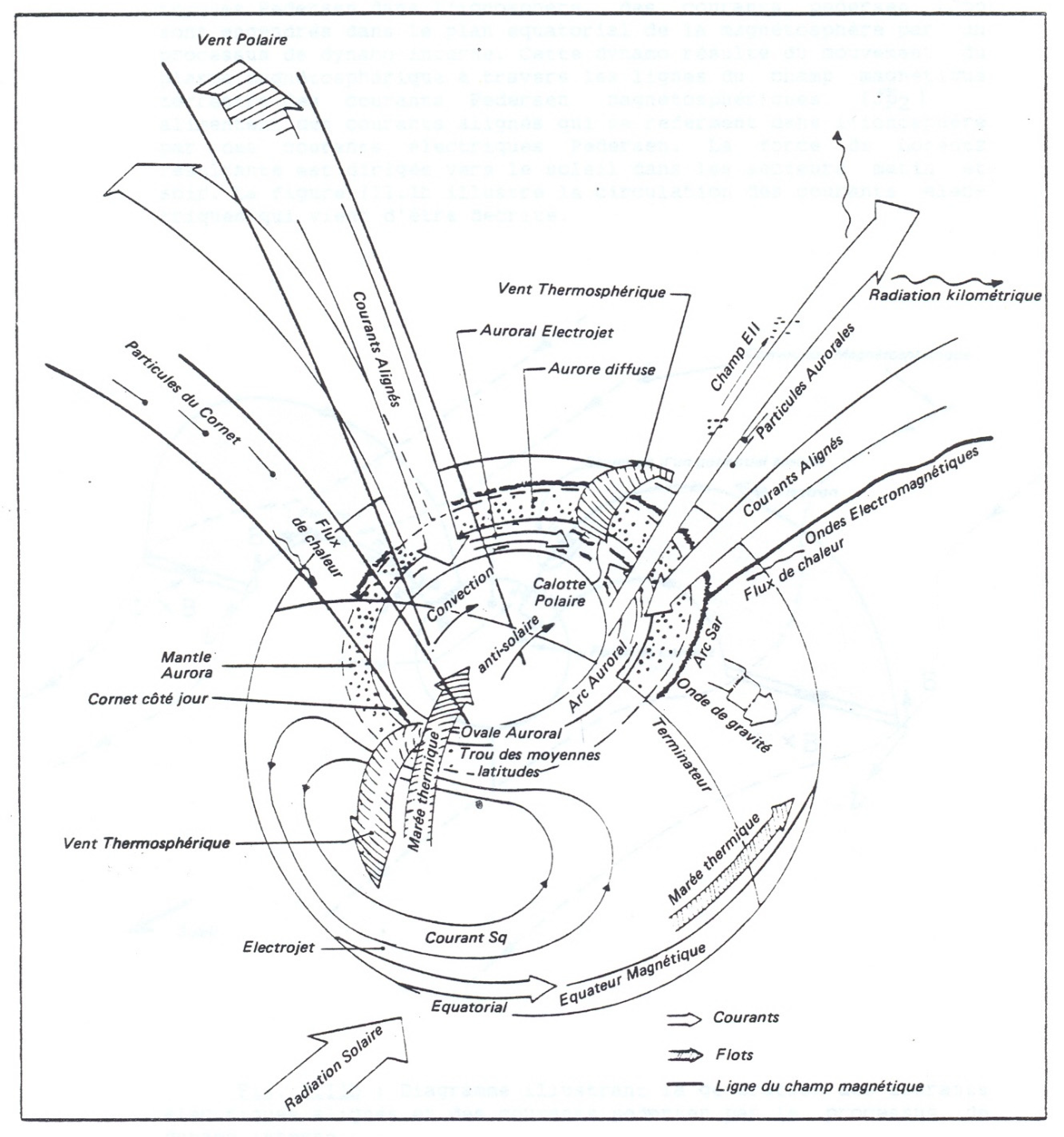
2.5. The Ionospheric Dynamo (External Geophysics)
Solar electromagnetic emissions (UV, X rays, EUV) ionize the atmosphere and are at the origin of different layers of the ionosphere (D, E, F) [
24]. In E layer (90–150 km), called the dynamo layer, ionospheric electric current flows on the dayside.
The neutral atmosphere dragging the ions through the lines of the Earth’s magnetic field under the effect of collisions is at the origin of the ionospheric electric currents. It is a dynamo effect at the origin of regular diurnal variations observed in the Earth’s magnetic field [
4], well-known as Sq and EEJ (equatorial electrojet), [
25,
26].
Figure 5 illustrates the variations of Sq and EEJ. During magnetic disturbed time, strong auroral electrojets also affect the middle and low latitudes through electrodynamic coupling between the high and low latitudes.
Table 1 brings together the values of the speed and magnetic field existing in the Sun–Earth system on a permanent basis and at the origin of the four large-scale permanent dynamos.
3. The Electric Currents and the Equivalent Electric Currents
There are very few electric current measurements in the terrestrial environment and the study of these electric currents is based on their signature on the Earth’s magnetic field [
28]. The real electric currents circulating in the terrestrial environment are three-dimensional, but the magnetic observations do not allow for three dimensions to be represented. The scientists of geomagnetism have zoned the Earth and derived systems of ‘equivalent’ currents to approach a complex reality. This approach is justified by the fact that the different electric current systems have different locations and the magnetic variations are very different from one location to another.
To derive from the observations an ‘equivalent current system’ that approximates ‘the real electric current system’, the equivalent current system needs assumptions about the geometry and properties of real electric currents, simplifying reality. However, the equivalent current system helps us to organize the magnetic observations on a planetary scale and gives a first rough approximation of the external electric currents
There are several regions for their magnetic effects of ionospheric electric currents, the auroral region, the middle latitudes, and the equatorial region where the equatorial electrojet circulates. The models used to derive the ‘equivalent current system’ are the model of a ribbon of current or the model of an infinite plane sheet of current above a plane Earth [
25]. At high latitudes, there are several ‘equivalent current system’ associated with the different polar disturbance, DP
1 [
29], DP
2 [
30], DP
3, and DP
4 [
31].
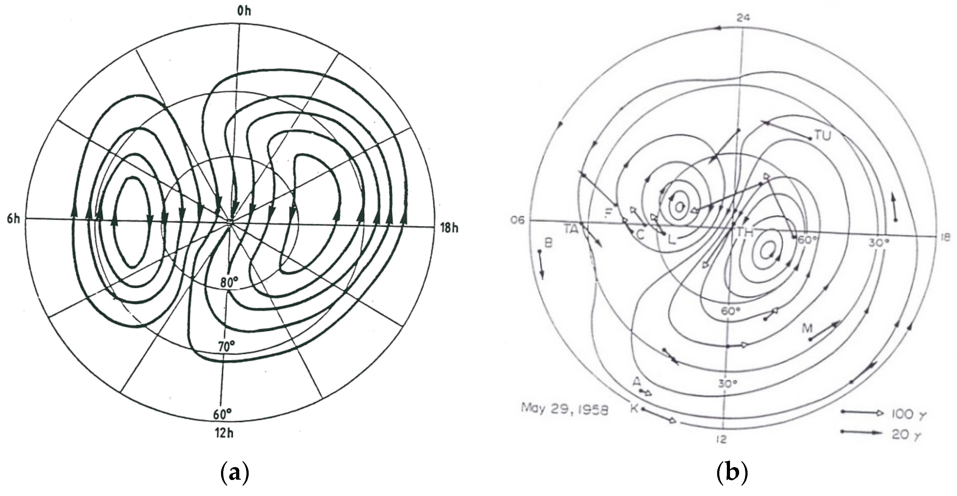
Figure 6 illustrates DP
2 [
30] and S
qP [
32]. The S
qP equivalent current system, confined at high latitudes, represents the effect of the solar wind magnetosphere dynamo during magnetic quiet periods. The DP
2 equivalent current system, extended to low latitudes, represents the effect of the solar wind magnetosphere dynamo.
The transmission of an electric field allows for the extension of the two cells of current from high to low latitudes [
30]. A first model developed in 1970 [
33] made it possible to represent these two current cells corresponding to the motion of particles. This is a model of prompt penetration of the magnetospheric electric field (PPEF).
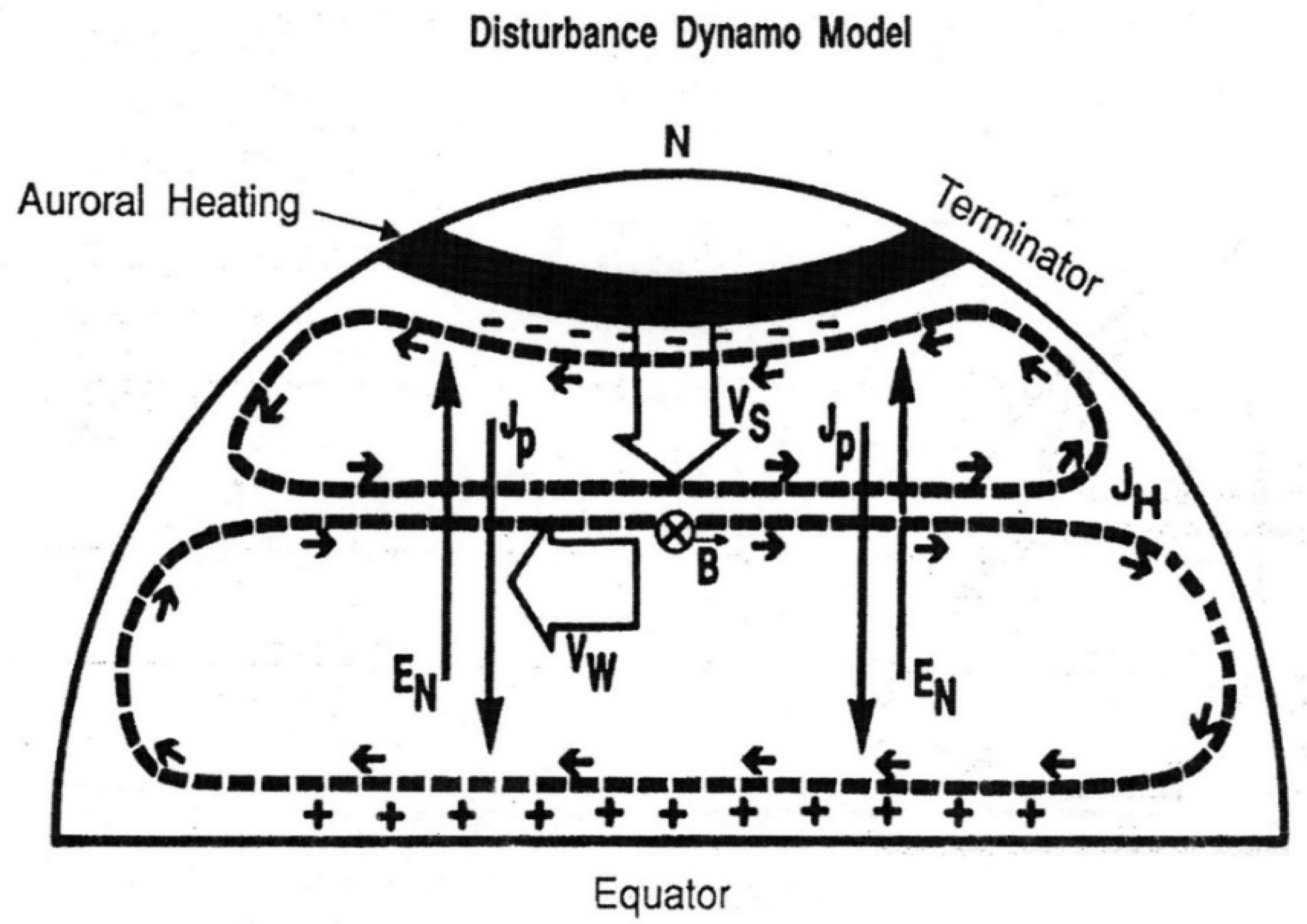
The auroral electrojets dissipate energy by Joule heating and produce movements of the thermosphere from high to low latitudes. These movements generate disturbed electric currents by the dynamo effect, which is the mechanism of the disturbed ionospheric disturbance dynamo [
6].
Figure 7 illustrates the model of the ionospheric disturbance dynamo [
7].
The Joule heating from the storm was assumed to extend uniformly around a high latitude zone. The southward meridional wind at the F region height arising from this heating is shown as the arrow VS. Due to the action of Coriolis force, the southward meridional produces a westward zonal motion (shown by arrow VW). The zonal motion of the ions, in combination with the downward component of the magnetic field (shown as x B), produces an equatorward Pedersen current (shown as JP). The Pedersen current builds up a positive charge at the equator until an electric field is established in the poleward direction opposing the flow of the Pedersen current. This poleward electric field is shown as EN. This electric field, which is perpendicular to the downward component of B, gives rise to an eastward Hall current with the maximum intensity in middle latitudes. This Hall current is marked as JH. The Hall current is interrupted at the terminators and gives rise to two current vortices, as shown. The lower latitude disturbance vortex is opposite in direction to the normal Sq current vortex.
In 1980, the ionospheric disturbance dynamo [
6] predicted a reverse of the electric current circulating at the equator, this current becoming westward, instead of eastward. This magnetic signature was found in 2005 on observations of the Earth’s magnetic field [
8]. This magnetic disturbance is not a polar disturbance type DP and it is named D
dyn 4. Estimation of the Magnetic Disturbance Ddyn Due to the Disturbance of Thermospheric Winds
Different steps are necessary to estimate the magnetic signature Ddyn of the ionospheric disturbance dynamo. We first need to characterize the different sources of electrical currents active in the Earth’s environment. Afterward, it is essential to know the physics of these different sources and the morphology of the electrical currents related to these sources, this is the second step. The third step is the analysis of the low latitude magnetic variations in order to detect strong Ddyn perturbation at these latitudes. Then, the use of signal technics allows us to isolate Ddyn, which is the last step.
4.1. The Different Sources of Electrical Currents in the Earth’s Environment, [28]
There are internal and external sources of electrical current in the Earth’s environment.
The Earth’s magnetic field expression is:
where B
p is the main field and varies from the equator (30,000 nT) to the pole (60,000 nT). B
a, the lithospheric magnetic field, is due to the magnetization of the Earth’s crust, and its amplitude varies from several nT to ~1000 nT. B
e is the magnetic field due to the electrical currents circulating in the ionosphere and the magnetosphere (qq nT to 2000 nT), which is related to external sources such as the ionospheric and solar wind/magnetosphere dynamos. Bin is the magnetic field due to currents induced by external sources (% of B
e) [
34].
During a space weather event (several minutes until several days), there is no variation in the main and lithospheric magnetic fields (ΔBp = 0 and ΔBa = 0). The Earth’s magnetic variations are due to external sources, ionospheric dynamo, and solar wind/magnetosphere dynamo.
4.2. Electrical Currents Related to External Sources
The variation in the Earth’s magnetic field is:
where S
R is a regular variation of the Earth’s magnetic field on a given day; Sq is the regular variation averaged on the five quietest days of a month; and D is the disturbance of the electrical currents during periods of magnetic activity.
The expression of the disturbance is [
35]:
where DCF is the disturbance due to Chapman Ferraro electric currents (magnetopause currents); DR is the disturbance due to the magnetospheric ring current; DT is the disturbance due to the magnetospheric tail currents; DI is the disturbance due to the ionospheric disturbed electric currents; and DG is the disturbance due to induced ground currents. All of these disturbances affect the Earth’s magnetic field (see
Figure 4 and
Figure 5 and the references concerning these figures). We know that the magnetic signature of the electric currents induced in the ground by the external electric currents has the same form, is weaker than the magnetic signature of the external electric currents, and it has become customary to consider the two sources of the internal and external magnetic fields together when we analyze magnetic variations.
The magnetic disturbance due to the ionosphere (DI) is the sum of all of the disturbed equivalent current system (Law of Biot and Savart). The expression of DI is:
where DP
1, DP
2, DP
3, and DP
4 are the polar disturbances. The magnetic disturbance D
dyn is not a polar disturbance. D
dyn is due to the Joule heating dissipated by auroral electrojets, (see the comment of
Figure 7). Only two equivalent current system, the DP
2 and the D
dyn, extend toward middle and low latitudes. The DP
2 disturbance is due to the magnetospheric convection electric field being more intense during the disturbed magnetic periods. This more intense electric field extends toward the middle and low latitudes.
Therefore, the expression of the disturbance D, at low latitudes is:
where D
iono is the part of DI affecting low latitudes, indeed DP
1, DP
3, and DP
4 are confined at high latitudes.
4.3. Variations in the Earth’s Magnetic Field at Low Latitudes
The electric currents circulating in the magnetosphere affect the low latitudes of Earth’s magnetic field, mainly the ring current circulating in the equatorial plane of the magnetosphere. Magnetic indices allow for the estimation of the magnetic disturbances due to these magnetospheric electric currents [
36,
37]. The use of SYM-H and ASYM-H is necessary to know the magnetic signature of disturbed ionospheric electric currents.
If we combine Equations (2) and (5), we obtain the variation in the H component of the Earth’s magnetic field at low latitudes:
We can estimate the regular variation (SR/Sq) from the Earth’s magnetic field observed during the magnetic quiet days preceding the magnetic storm, and the magnetospheric electric currents from the magnetic indices SYM-H and ASYM-H. Therefore, it is possible to quantify Diono.
4.4. Estimation of Ddyn
By signal processing, we can separate the contributions of DP2 and Ddyn. This opens up many possibilities for studying the signature of the disturbed ionospheric dynamo that affects the circulation of electric currents at the equator.
To extract D
dyn, the simplest method is to select very quiet days just after a storm [
8], no more auroral activity, no more DP
2 disturbance, and D
iono is directly D
dyn. These cases are rare, and therefore different signal processing techniques are necessary to extract D
dyn [
34,
35,
36]. To separate the DP
2 and D
dyn magnetic disturbances, different techniques have been used: (1) average over four hours with a sliding step of one hour, which makes it possible to eliminate periods of less than 3 hours concerning the DP
2 disturbance [
38]; (2) wavelet analysis [
39]; and (3) wavelet analysis with semblance [
40]. We present here in
Figure 7 and
Figure 8 the results of the last method used [
40].
Table 2 gathers all the useful elements to evaluate the magnetic disturbance associated with the disturbance of the thermospheric winds and are described in the previous parts.
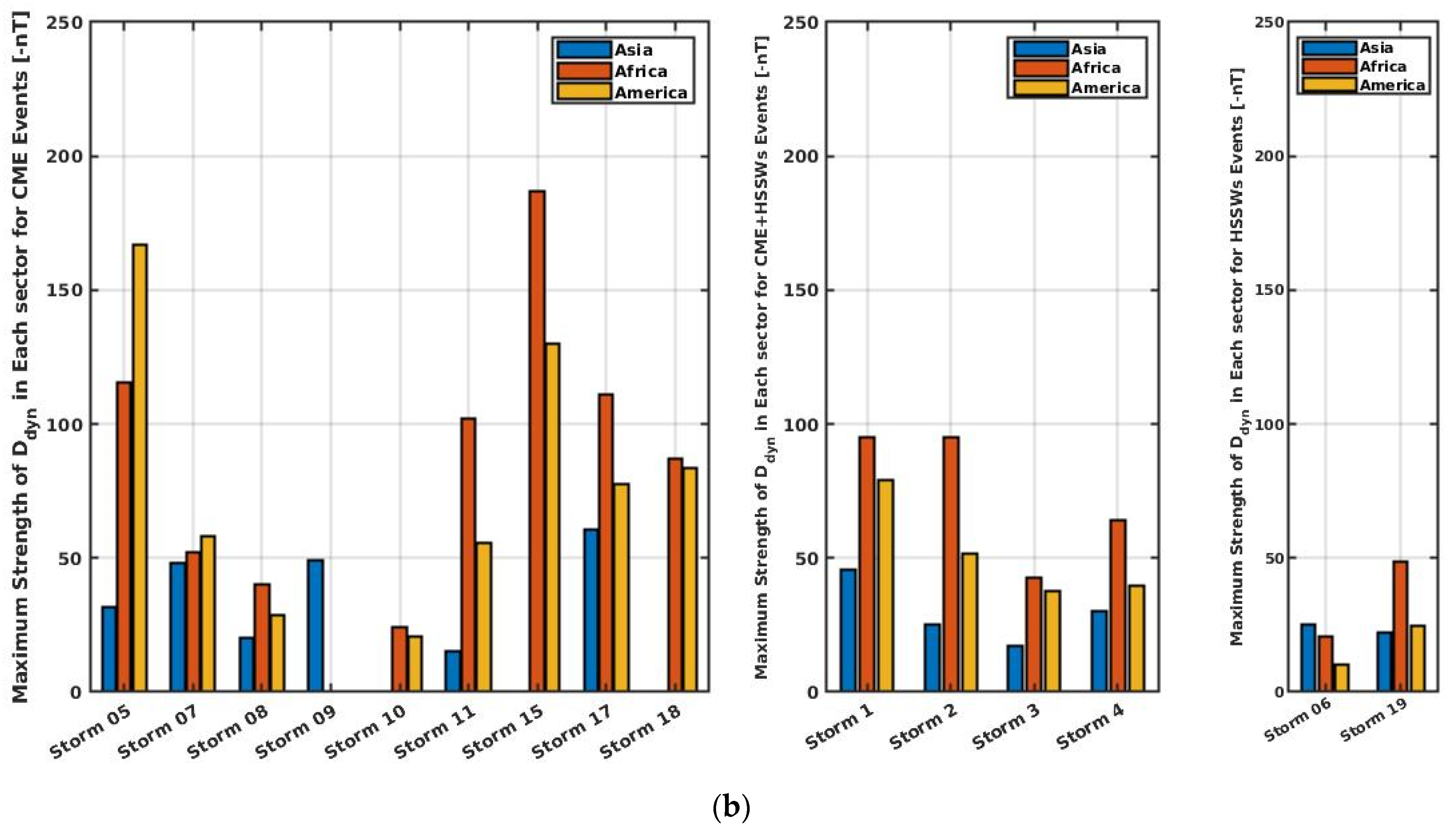
Figure 8a,b [
40] illustrate the D
dyn magnetic signature obtained for 19 storms.
Figure 8a presents the maximum duration of D
dyn in days and
Figure 8b shows the maximum value of D
dyn in nT, in the three sectors of longitude Asia, America, and Africa. We classified the geomagnetic storms into three categories storms, due to CME (coronal mass ejection) or due to CME + HSSW (high speed solar wind) or a sole HSSW. We found that the strongest values (~200 nT) were observed when there was a CME, and the longest duration when there was a HSSW (5 days) associated or not with a CME. We also observed a difference of D
dyn according to the longitude. One notes that for some CME, the magnetic disturbance D
dyn affects only one or two longitude sectors. On the other hand, when there is a HSSW, all longitude sectors are affected. The fact that certain longitude sectors were not affected by the magnetic disturbance D
dyn is related to the duration of the Joule heating in the auroral zone. Indeed, if the Joule heating associated with a CME has a short duration of several hours, the thermospheric wind disturbance affects one or two sectors of longitude. In the case of HSSW, the disturbance of the Joule heating in the auroral zone lasts several days and thus all longitude sectors are affected by the thermospheric wind disturbance and its associated magnetic disturbance D
dyn.
5. Conclusions
Recently, a very useful review on the ionospheric dynamo was published [
41], necessary to stop the loss of knowledge. Currently, many young scientists are studying in the equatorial zone without having the necessary knowledge, so sometimes the variations in the ring current observable at the magnetic equator are interpreted as a counter-electrojet (CEJ). Some physical phenomena have similar magnetic signatures [
42], which is why it is necessary to make a systemic analysis of the Sun–Earth system to fully understand the processes acting in this global system in order to interpret the variations in the observed Earth’s magnetic field. In conclusion, this article brings together the essential knowledge of physics to understand and analyze the magnetic disturbance generated by the disturbed thermospheric winds during magnetic storms.
In this article, we have presented the need to know the global context of the Sun–Earth system to study the variations in the Earth’s magnetic field. We have more particularly presented the magnetic signature (D
dyn) of the process of an ionospheric disturbed dynamo [
6,
7,
8], which generates the average magnetic activities that persist for several days after a storm [
33,
34]. During the last decade, we have refined the signal processing methods to extract this magnetic disturbance D
dyn [
33,
34,
35].
During the last decades, the physics of the Sun has greatly progressed thanks to satellites such as SOHO, which has made it possible to develop space weather. Indeed, the solar physicists classified the various solar disturbances, particularly the HSSW flowing from solar coronal holes. Previously, physicists of the ionosphere selected the effect of the solar disturbances, showing a strong variation in the storm magnetic index Dst and they selected mainly CMEs. Indeed, the HSSW disturbs the electromagnetic environment of the Earth, but in general, does not have a strong signature on the magnetic index Dst, sometimes no more than 50 nT. The development of space weather has allowed for progress in the study of the impact of HSSW on the electromagnetic environment of the Earth, and consequently, the understanding of average magnetic disturbances not previously well understood.


