Bias Correction and Evaluation of Precipitation Data from the CORDEX Regional Climate Model for Monitoring Climate Change in the Wadi Chemora Basin (Northeastern Algeria)

Abstract

This study aims to provide a brief overview of four regional climate model (RCM) estimations for (Daily, Monthly, Seasonal, and Annual) averaged precipitation over the Wadi Chemora Basin in northeastern Algeria for the historical period (1970–2005) and future forecasts (2006–2100). Data from seven ground stations were compared to data from four RCMs: RCA4 driven by ICHEC-EC-EARTH and NOAA-GFDL-GFDL-ESM2M from MENA-CORDEX domain with intermediate resolution (25 km, 0.22°) and ALADIN and RegCM4 from MED-CORDEX domain with high resolution (12 km, 0.11°). In most time steps (Annual, Seasonal, Monthly, and Daily), the raw RCMs overestimated precipitation, but their performance improved significantly after applying gamma quantile mapping (GQM) bias correction method. The bias-corrected projections indicate decreases of seasonal rainfall for the near future (2010–2039), mid-century (2040–2069), and end of century (2070–2100) periods. Overall decreases in all seasons lead to the projected decrease in annual rainfall of an average of 66% by the end of the 21st century.

1. Introduction

There is overwhelming evidence that human activity is contributing to the uptick in climate extremes and rising concentrations of greenhouse gases (GHGs) [1,2,3,4]. As a result, the earth is plainly warming, and climate change is reshaping life on our planet in a variety of ways. Some places have been harmed by rising sea levels [5,6,7,8], while others have been impacted by extreme weather events, such as droughts or floods [9,10,11,12]. Precipitation, which is the key player and driver in these extreme occurrences, has been directly affected by climate change; wet areas becoming wetter, especially in the mid-to-high latitudes, and dry areas becoming drier (generally throughout the subtropics) [13]. According to several studies, the Mediterranean Basin is one of the areas most vulnerable to a substantial reduction in total precipitation [14,15,16,17,18,19]. This region which stretches from the arid subtropics to the temperate mid-latitudes is already characterized by low annual precipitation totals and considerable interannual variability, resulting in semipermanent water stress, especially in the south, where precipitation has plummeted dramatically in North African countries [20,21,22,23]. Algeria is one of these countries that have been suffering from prolonged drought for more than three decades [24,25,26,27,28]. Therefore, examining climate change and its influence on precipitation, as well as producing trustworthy high-quality estimates of future changes across the country and on a regional scale, has become an absolute requirement.

To attain this requirement, we must rely on climate models since they are our only tools peering into the future and looking forward to assessing the likely ranges of possibilities. We cannot actually run more than one experiment on the real planet Earth, meanwhile climate models allow us to try out all sorts of (what-if) scenarios and observe what occurs. Over the last few decades, climate modeling groups have significantly improved the simulations of general circulation models (GCMs) [29,30,31,32]. These models describe the response of the global circulation to large-scale forcing effects, such as anthropogenic (e.g., greenhouse gas emissions) and natural (e.g., solar output and volcanic activity) influences and estimate future global climate. However, multiple researchers have raised concerns about biases and uncertainties in these models’ simulations, and notably their poor performance in precipitation modeling in complex topographical regions [30,33,34,35].

Therefore, different downscaling approaches have been developed to alleviate GCM deficiencies. These downscaling methods are classified into two types: statistical and dynamical. Statistical downscaling approaches estimate higher resolution climate data by building statistical relationships between low resolution climatic or atmospheric data and locally observed data [36,37]. While in dynamical downscaling methods, local-scale climate is estimated by nesting a mesoscale higher resolution model or regional climate model RCM within a GCM. RCM is driven to simulate local scale processes over a smaller region using finer grids by lateral boundary conditions from GCM output to predict better resolution climate while taking into account biogeophysical interactions occurring at the land–atmosphere interface within the grid [38,39,40]. Dynamical downscaling with regional climate models is a more physically realistic approach than statistical downscaling [41,42]. The international regional downscaling community called Coordinated Regional Climate Downscaling Experiment (CORDEX) initiative has made available an enormous amount of regional climate projections in different domains worldwide [43]. However, on the other hand, RCMs may still yield considerable systematic errors [44,45,46,47] prohibiting the direct use of simulated output unless it has been corrected for regional and local climate impacts and adaptation studies [48,49,50,51,52,53,54,55,56]. In the last decade, many bias correction methods have been developed, ranging from simple scaling (linear scaling) to sophisticated distribution mapping [57,58,59,60,61,62,63]. Several studies have proven that quantile mapping approaches (both parametric and nonparametric) are effective for correcting RCM-simulated precipitation [56,57,60,64,65,66,67], which we thus we applied in our work.

In Algeria, the use of climate models in general, and regional models in particular, to investigate climate change impacts is quite limited (e.g., References [55,56,68,69,70,71]), with the majority of these studies focusing on the country’s west. Therefore, in this work, we draw attention to the east, namely the northeast of Algeria, where the Chomora basin is located. The objective is to examine the significance and efficacy of gamma quantile mapping (GQM) bias correction on RCM model outputs over the mentioned study domain, as an intermediate step before performing any regional impact analysis. The remaining section of the paper is organized as follows: Section 2 highlights the data and methods used, while results and discussions are presented in Section 3. The last section summarizes the conclusion of the study.

2. Materials and Methods

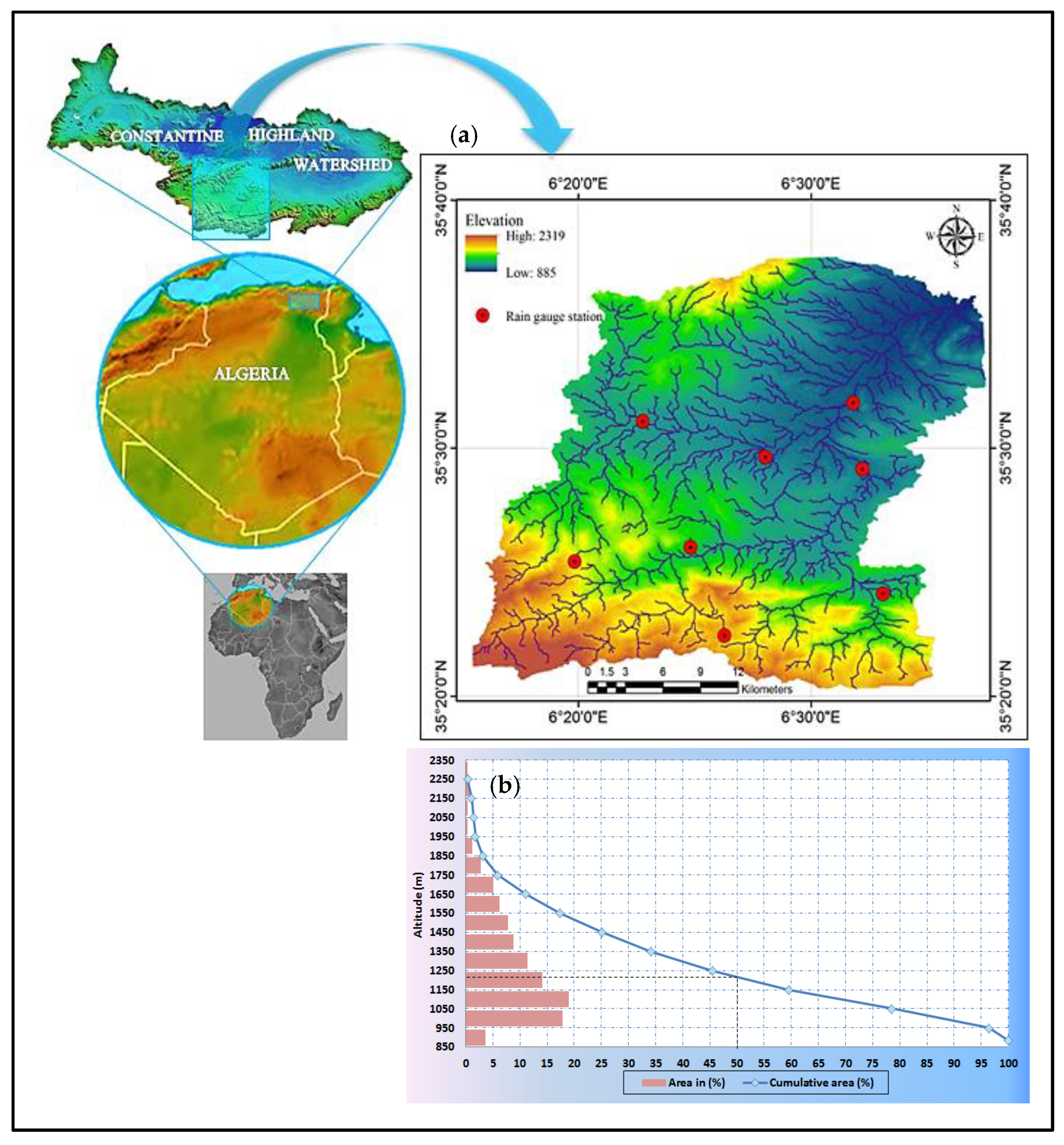
2.1. Study Area

Wadi Chemora Basin with an area of 751.6 km² is part of the large watershed of Constantine highland. It is located in northeastern Algeria between 6°15′ and 6°40′ of eastern longitude and 35°20′ and 35°38′ northern latitude (Figure 1a) at the foothills of the Aures Mountains in the Wilaya of Batna. It features a rugged topography with heights ranging from 885 m at its outlet to 2319 m at El Mahmal Mountain’s summit and more than 50% of the entire region lies above 1200 m as shown in the hypsometric curve (Figure 1b). The region’s geologic formations are stable: Quaternary glacis (27%), Turonian sandstone (16%), and middle Cretaceous wooded limestone marls dominate the basin’s south (10%). The lower basin of Chemora is dominated by Quaternary layers, sandstone formations, and siliceous clays [72,73]. The main tributary of Wadi Chemora is around 37 km long and is formed by the junction of two streams (Reboa and Soultez). It flows from the southwest to the northeast until draining into the salt lakes of Constantine’s highlands, which serve as its hydrological outlet. The hydrological regime of the Wadi Chemora mostly depends on the rainfall regime. It is distinguished by considerable spatio-temporal variability, with a succession of periods of high and low water levels. The average interannual flow recorded at the Chemora station, which controls the entire basin, is estimated to be 0.72 m³/s over the observed period from September 1969 to August 2005 (according to collected data from National Agency of Water Resources. Algiers (NAWR) 2017).

The study area has a semi-arid Mediterranean climate that conforms to Köppen’s climatic classification description of this kind of climate, with hot, dry, sunny summers and cold, rainy winters [68]. The monthly temperature averages collected from Batna meteorological station over a 31-year period (1984–2014) show that the region’s lowest average temperature is in January (6.9 °C) and the highest is in July (27.0 °C), with a substantial amplitude between the lowest value of the average of minimums (0.2 °C) and the highest value of the average of maximums (35 °C). The average interannual of precipitation in the basin for the period 1970–2005, varies from less than 280 mm in the northeast to more than 550 mm in the south, with an average estimated at 334 mm [Author’s own elaboration based on NAWR data, 2017]. According to Guidoum et al. (2012), the precipitation for the period 1969–2004 reveals a deficit that can reach 20% compared to the data from the 1913–1963 series of CHAUMANT and PAQUIN [61], which underlines the importance of investigating the impact of climate change on precipitation in this region.

2.2. Data Description

The data sources in this study are of two types: Rain Gauge Dataset and Regional climate model output. The Rain Gauges are seven observed data collected within Wadi Chemora basin (Figure 1a), the eighth station in this figure is Koudit Mdour with the code (070411), which is omitted from our study since its data begins in 2004; those data were obtained from the National Agency for Water Resources (NAWR) of Algeria (

Table 1. Precipitation Gauge stations.

Code	Station Name	Lat °	Lon °	Alt (m)	Period
070403	Reboa	35.29	6.32	1002	Sep 1969–Dec 2005
070405	Ain Tinn	35.22	6.26	1650	Sep 1969–Feb 2014
070406	Foum Toub	35.24	6.33	1160	Sep 1969–Aug 2013
070407	Baiou	35.25	6.19	1510	Sep 1969–Feb 2014
070408	Bouhmar	35.26	6.24	1275	Sep 1969–Sep 2012
070409	Timgad	35.29	6.28	1000	Sep 1969–Feb 2014
070410	Sidi Macer	35.31	6.22	1112	Sep 1969–Feb 2014

). The RCMs precipitation data were sourced from two domains of (CORDEX): the Middle East and North Africa domain (MENA) with intermediate resolution (25 km, 0.22°) and the Mediterranean domain (MED) with high resolution (12 km, 0.11°). The four (4) RCMs that we examined are as follows: from MENA we selected RCA4 driven by two GCMs: ICHEC-EC-EARTH and NOAA-GFDL-GFDL-ESM2M while from MED: ALADIN and RegCM4 (

Table 2. Regional climate models (RCMs) used in this study.

CORDEX Domain	Resolution	Institution	Driving Model	CMIP5 Experiment	RCM Model
MENA-22	Intermediate resolution (25 km, 0.22°)	SMHI	ICHEC-EC-EARTH	Historical rcp85	NOAA-RCA4
			NOAA-GFDL-GFDL-ESM2M	Historical rcp85	ICHEC-RCA4
MED-11	high resolution (12 km, 0.11°)	CNRM	CNRM-CM5	Historical rcp45 rcp85	ALADIN
		ICTP	ICTP-RegCM4	Historical rcp85	RegCM4

).

Since the datasets in this study are from two distinct CORDEX initiatives with different resolutions, they are first interpolated into the lowest spatial resolution (0.22°).

In regions with sparse distribution of rain gauge networks and complex topography, the accuracy and precision of interpolation to assess grid measurements for a climate model is questioned [74,75].

Therefore, due to the sparse station network in Chemora basin, we use the point (station) to pixel approach to interpolate the grid data of RCMs to the stations locations. This method is commonly used to compare ground observations with other data products, such as satellite-based rainfall estimates and climate model outputs, e.g., [76,77,78,79,80].

The RCMs provide historical data and forecast the future using several “Representative Concentration Pathways” RCPs. In this analysis, we focus on the low to moderate future emissions scenario (RCP 4.5) and the worst-case scenario of high emissions (RCP 8.5). The historical data are considered for the period 1970–2005 (adjusted to the period of available observations). For future projections the RCP8.5 scenario is considered in the period 2006–2100 except for RegCM4, which projects from 2006 to 2099.

2.3. Bias Correction Method

The focus of the study is to evaluate the performance of the bias adjustment of multiple RCMs output (precipitation). The raw outputs of the four (4) RCMs are obtained in the form of NetCDF files and from this gridded RCM model data, a representative value for each rain gauge station was extracted by using Climate Data Operator CDO.

The “bias correction” refers to the process of rescaling climate model output to minimize the impact of systematic errors in climate models [81]. The core concept of this process is the detection of potential biases between observed and simulated climatic variables, which serves as the foundation for correcting both control and scenario RCM runs using a transformation algorithm. Precipitation is the main variable subjected to bias correction in this study. Typically, for transforming modelled precipitation ($P_{mod}$) to match the observed data ($P_{obs}$), the bias correction methods adjust the mean, variance and/or distribution of the modelled precipitation by using a function h as shown in Equation (1) [82].

$$P_{obs}=h\left(P_{mod}\right)$$

(1)

In this work, we apply the gamma quantile mapping GQM method to daily precipitation, since, as we mentioned in the introduction above, it has been demonstrated by so many studies that it is an effective approach for correcting RCM-simulated precipitation. The concept behind distribution mapping is to correct the distribution function of RCM-simulated climatic values by establishing a transfer function that shifts precipitation occurrence distributions to accord with the observed distribution function [60,83] with assumption that both the RCM simulated and observed precipitation follow a specific frequency distribution [84]. It is used to adjust the mean, standard deviation, and quantiles.

So, the relation in Equation (1) can be reformed so that the distribution of the modelled precipitation matches that of the observations:

$$P_{obs }=F_{obs }^{-1}\left(F_{mod }\left(P_{mod}\right)\right)$$

(2)

where $F_{mod }$ is the cumulative distribution function (CDF) of $P_{mod}$ (modelled precipitation) and $F_{obs }^{-1}$ is the inverse CDF corresponding to $P_{obs }$ (observed precipitation). These CDFs can either be theoretical distributions fitted to the data or empirical distributions estimated by sorting the data. The gamma distribution with shape parameter α and a scale parameter β (Equation (3)) is commonly used to characterize the CDF of precipitation [57,60] and the method is termed as gamma quantile mapping GQM:

$$f\gamma \left(x|\alpha ,\beta \right)=x^{\alpha -1}·\frac{1}{{\beta }^{\alpha }·\mathsf{\Gamma }\left(\alpha \right)}·e^{\frac{-x}{\beta }}; x\ge 0; \alpha ,\beta >0$$

(3)

Note that $f\gamma$ is the gamma CDF (cumulative distribution function), $\mathsf{\Gamma }( )$ is the gamma function and $x$ is normalized precipitation. The distribution profile is controlled by the shape parameter α in three ways: (1) if α < 1 signifies an exponentially shaped Gamma distribution, which is asymptotic at both axes, (2) α = 1 particular case that denotes an exponential distribution and (3) α > 1 shapes a skewed unimodal distribution curve. The Gamma distribution’s dispersion is determined by the scale parameter $\beta$. The bigger the $\beta$, the greater the dispersion stretched of the distribution, and hence the greater the probability of the occurrence of extreme events; conversely, the lower the $\beta$, the more compacted the distribution’s dispersion, and thus the lower the probability of extreme occurrences [60]. Bias correction method is assumed to be stationary, i.e., the correction algorithm and its parametrization for current climate conditions are assumed to be valid for future conditions as well. Thus, the same correction algorithm is applied to the future climate data [60,85].

It should be noted that the four RCMs simulate too many days with very low precipitation and not enough dry days (many drizzle days). Therefore, in an initial step, we adjusted the number of simulated dry days in the RCM simulations to match the number of observed dry days by including a wet day threshold and replacing all values below it with zero. More information about these found in Teutschbein and Seibert (2012) [60] and Fang et al. (2015) [86].

2.4. Spatial Analysis

The spatial pattern of observed and simulated (Raw RCMs and bias corrected (BC) RCMs) the precipitation of annual averaged and seasonal averages was obtained by interpolating precipitation from seven stations in the Wadi Chemora Basin using the inverse distance weight (IDW) method. This method interpolates average precipitation using latitude, longitude, and a gauging station’s average precipitation, so it is based on spatial and temporal structure. Several studies, e.g., [87,88,89,90] have found that the results of IDW interpolation for averaged precipitation are very accurate with a reasonable calculation. The IDW interpolation for estimating precipitation is given in Equations (4)–(6) [91].

$$P_P={\displaystyle \sum }_{i=1}^N{W}_i{P}_i$$

(4)

$$W_{i }=\frac{d_{pi}^{-m}}{{{\displaystyle \sum }}_{i=1}^N{d}_{pi}^{-m}}$$

(5)

$$P_{P }=\frac{{{\displaystyle \sum }}_{i=1}^N{P}_i{d}_{pi}^{-m}}{{{\displaystyle \sum }}_{i=1}^N{d}_{pi}^{-m}}$$

(6)

where P_p denotes the required precipitation data in (mm) and P_i is the precipitation data from the gauging station in (mm), The weighting of individual precipitation stations is represented by W_i, N is the number of gauging stations, d_pi is the distance from each station to the required point, m is the exponent, and the controlling factor fixed by the user and usually assumed to be 2 [87].

2.5. Evaluation of Bias Correction Approach

The performance of the GQM correcting method regarding the historical simulations of precipitation datasets was evaluated in different time steps (Annual, Seasonal, Monthly, and Daily) utilizing raw and bias-corrected RCMs against the observed precipitation gauge dataset in our study area. For a statistical evaluation, we use a Taylor diagram that can summarize several statistical characteristics. This mathematical diagram was developed by Karl E. Taylor in 1994 (published in 2001 [92]), it depicts the statistical connection between two fields, a “test” field (typically representing a field simulated by a model) and a “reference” field (normally representing “truth” based on observations). Each point in the 2D space of the Taylor diagram may represent three separate statistics at the same time (spatial correlation coefficient of Pearson R, the root mean square error RMSE, and the standard deviation σ) because these statistics are related by the following formula (for given “test” field (f) and a reference field (r)) [92]:

$$CRMSE²={\sigma }_f^2+{\sigma }_r^2-2{\sigma }_f{\sigma }_{r}R$$

(7)

where CRMSE is the centered RMSE between the fields:

$$RMS{E}^2=CRMS{E}^2+\left(\overline{f}-\overline{r}\right)²$$

(8)

Considering two variables, $f_i$ and $r_i$, which are defined at N discrete points (in time and/or space), $\overline{f}$ and $\overline{r}$ are the mean values; R is the spatial correlation coefficient given by the following Equation:

$$R=\frac{\frac{1}{N}{{\displaystyle \sum }}_{i=1}^N\left(f_i-\overline{f}\right)\left(r_i-\overline{r}\right)}{{\sigma }_f{\sigma }_r}$$

(9)

The standard deviations of the “test” field (σ_f) and the reference field (σ_r) fields are provided below:

$${\sigma }_f=\sqrt{\frac{1}{N}{\displaystyle \sum }_{i=1}^N\left(f_i-\overline{f}\right)²}$$

(10)

$${\sigma }_r=\sqrt{\frac{1}{N}{\displaystyle \sum }_{i=1}^N\left(r_i-\overline{r}\right)²}$$

(11)

A perfect score is obtained when the model mark and the observation mark match, signifying complete correlation, zero RMSE, and equal standard deviation [92].

2.6. Analysis Future Projections

In this section, the Mann–Kendall trend test was used to examine the future trend of the four RCMs over the entire period (2006–2100 (or 2099)) with respect to the historical period (1970–2005). The future period was then divided into three sub-periods: near (2010–2039), medium (2040–2069), and long term (2070–2100). The annual and seasonal anomalies (delta change in %) with respect to the baseline climate (1970–2005) of the same RCM before and after bias correction were compared for each future period.

Mann–Kendall Trend Test

The Mann–Kendall test is based on the calculation of Kendall’s tau measure of association between two samples, which is itself based on the ranks of the samples. This method is a non-parametric rank-based procedure that has been commonly used to assess if there is a trend in a time series hydro-meteorological data [93]. The Mann–Kendall test was applied to test trends in future climatic variables. Mann–Kendall test is expressed by Equations (12) and (13). X₁, X₂, …, Xn represent n data points where X represents the data point at time j. The Mann–Kendall statistic (S) is given by Equation (12):

$$S={\displaystyle \sum }_{k=1}^{n-1}{\displaystyle \sum }_{j=k+1}^{n}sign \left(X_j-X_k\right)$$

(12)

$$\mathrm{For}:sign\left(X_j-X_k\right)=\{\begin{array}{c}1 if \left(X_j-X_k\right)>0\\ 0 if \left(X_j-X_k\right)=0\\ -1 if \left(X_j-X_k\right)<0\end{array}$$

(13)

A positive value of S is an indicator of an increasing trend and a negative value indicates a decreasing trend.

3. Results and Discussion

3.1. Historical Simulation before and after Bias Correction

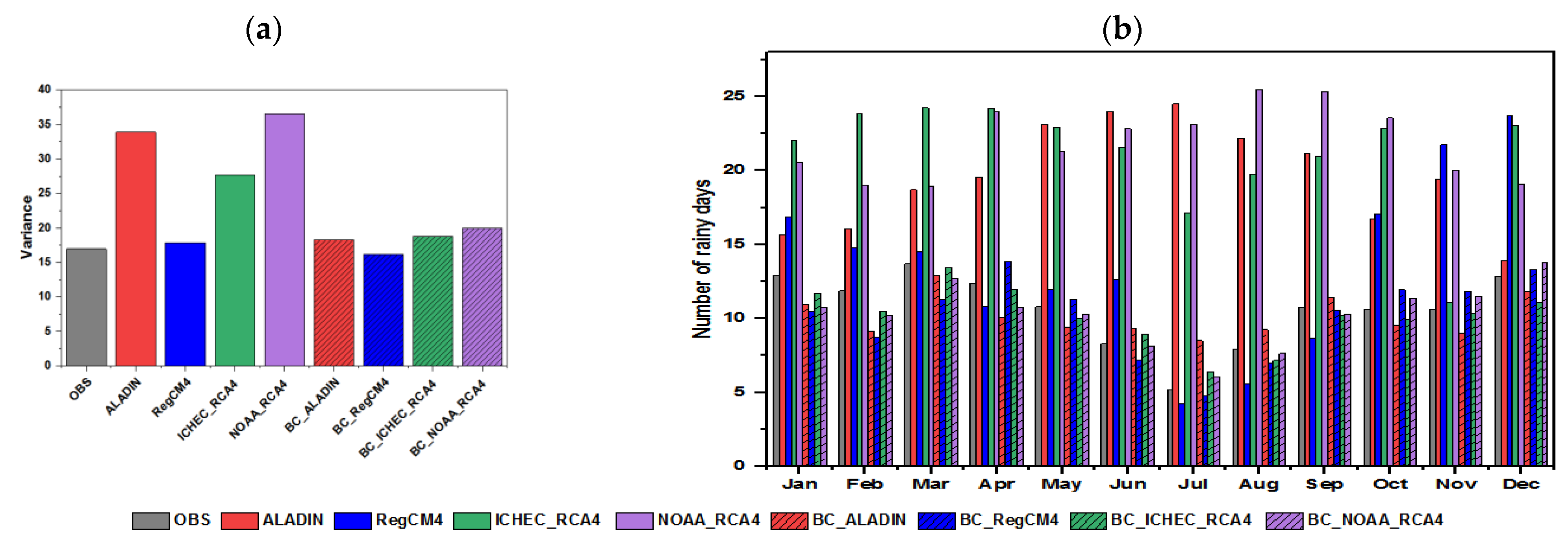
This section provides visual assessments by comparing observed and simulated precipitation at-site (individual rain gauge stations) and areal-averaged precipitation in different time steps (Daily, Monthly, Seasonal and Annual) over the historical period (1970–2005).

3.1.1. Daily Scale

The Half Box–Scatter plots of raw, corrected RCMs, and observational annual cycle of daily precipitation over (1970–2005) for the seven rain gauge stations in Wadi Chemora Basin presented in Figure 2 shows that before the bias adjustment most models overestimated the daily precipitation in most stations. Regarding the raw outputs of the two MED models, ALADIN showed a higher overestimation in all stations, whereas RegCM4 showed a lower overestimation in most stations and even underestimated precipitation in Ain Tinn and Foum Toub stations. As for the MENA models ICHEC-RCA4 and NOAA-RCA4, we noticed an obvious bias and significant overestimation of daily precipitation at higher altitudes (from 1160 m to 1650 m) stations, such as Baiou station, which is located at an altitude of 1510 m; while it performed better at lower elevations (from 1000 m to 1112 m) stations, such as Reboa station with a height of 1002 m. Some recent studies, e.g., [94,95], indicated that the performance of RCM can be dependent on elevation. According to those studies using RCA4 from the Africa domain (AFR) and the Middle East and North Africa domain (MENA) with (0.44° resolution), showed good performances in low-elevation regions, this was confirmed in this study for RCA4 with a higher resolution in Wadi Chemora Basin. Consistent with many studies applying GQM method [56,60,86], the outputs of all models, regardless of their performance, have been effectively adjusted by this method, as shown by the good correspondence between median values of the models and observed daily precipitation, as well as the fact that the data distribution improved significantly after bias correction (Figure 2).

The temporal characteristics of the observed and simulated variance over the period of (1970–2005) (Figure 3a) and the number of rainy days with rainfall magnitude above 0.1 mm (definition of a light rainy day as per Algeria Meteorological Department) during each month (long-term monthly average) before and after bias correction (Figure 3b) were compared to assess the performance of the RCMs.

Figure 3a shows that after correcting the biases, the variance of all models approaches the variance of observed data.

The analysis of the total number of rainy days simulated in a year (over a 36-year simulation period (1970–2005)) by the four RCMs (Figure 3b) reveals significant differences in the average number of rainy days simulated before adjusting the models (all models overestimate the average number of rainy days) compared to the total number of rainy days observed. After bias correction, the differences shrink and the average number of rainy days of RCMs approach the average number of rainy days observed.

3.1.2. Monthly Scale

Figure 4a shows a line graph plot and Figure 4b shows a heatmap plot; demonstrating the areal-averaged monthly precipitation cycle for observed and simulated (Raw and adjusted RCMs) across the Wadi Chemora Basin region from 1970 to 2005. The raw (uncorrected) RCMs had significant discrepancies in their ability to recreate monthly precipitation and showed biases, such as the overestimation of precipitation and misrepresentation of rainy season timing.

According to the observed data, the summer months of June, July, and August (JJA) (the dry season of the year in the study region) are the least rainy, yet before bias adjustment, the ALADIN model from MED and the NOAA-RCA4 model from MNA assessed them as the rainiest months. The overestimations of rainfall by these models during JJA appear to be consistent with some studies in North Africa [56,96].

ALADIN, in particular, greatly overestimated precipitation in the majority of months, especially in July, where it considered it to be the rainiest month with a value of 133.2 mm, when in fact, it is the least rainy month in the region, with an average value not exceeding 7.55 mm. However, this model showed a better performance in estimating December precipitation before and after bias correction consistent with the findings in other studies [56,96,97]. Prior to bias adjustment, the RegCM4 model from MED largely succeeded in simulating the precipitation the three months of Mars, April, and July compared to observed data but underestimated it in August and September and overestimated it in the remaining months of the year [98]. The raw ICHEC-RCA4 data from MENA are almost consistent with the observed precipitation in November but overestimate precipitation in all other months [99].

However, before the bias correction, these latest two models performed better in terms of rainy season timing than the previous two models mentioned above, which is consistent with other studies [100,101].

After bias adjustment, the areal-averaged monthly precipitation of the RCMs simulated over the historical period (1970–2005) was considerably improved and mostly agreeed with the observed data.

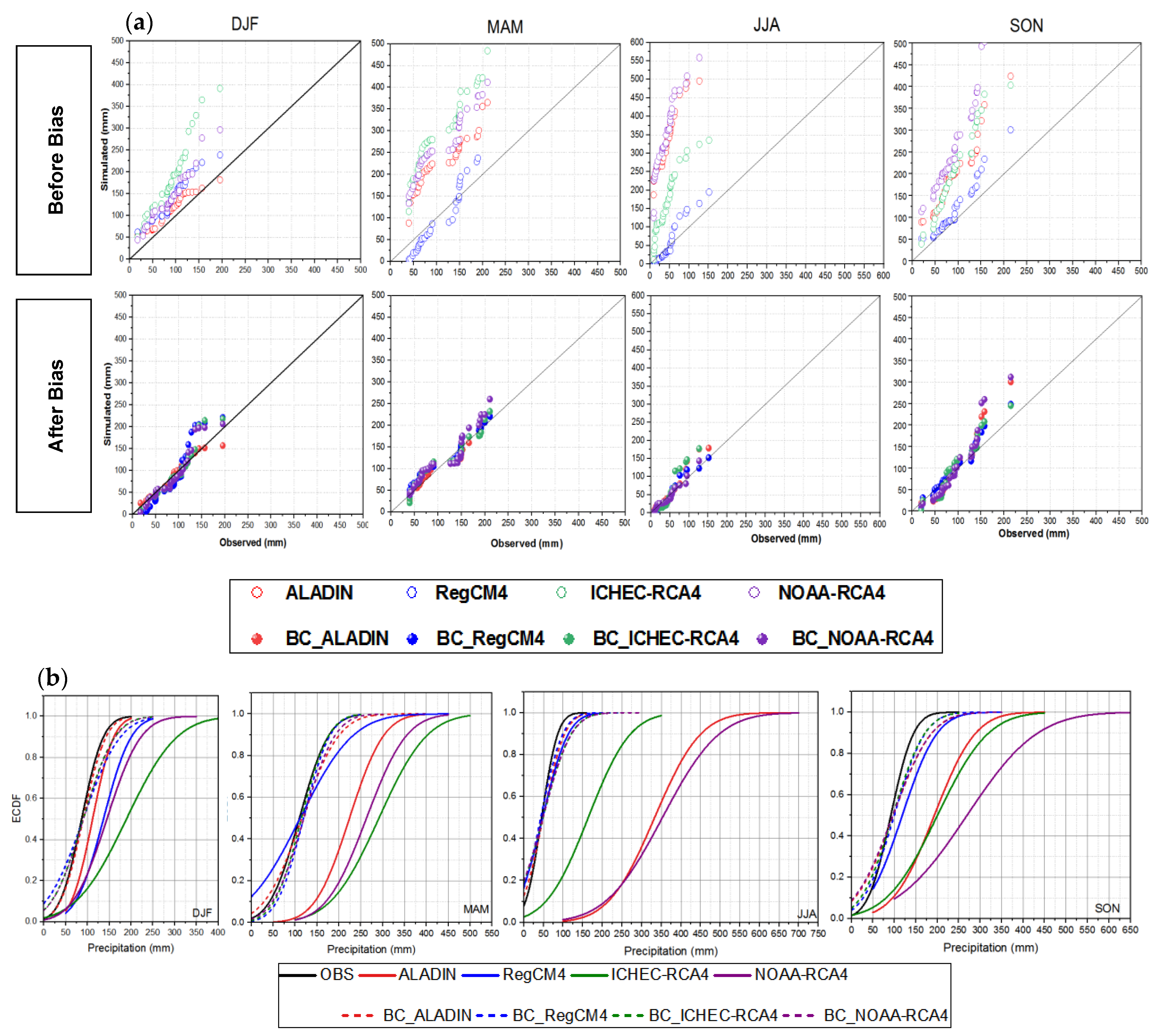
3.1.3. Seasonal Scale

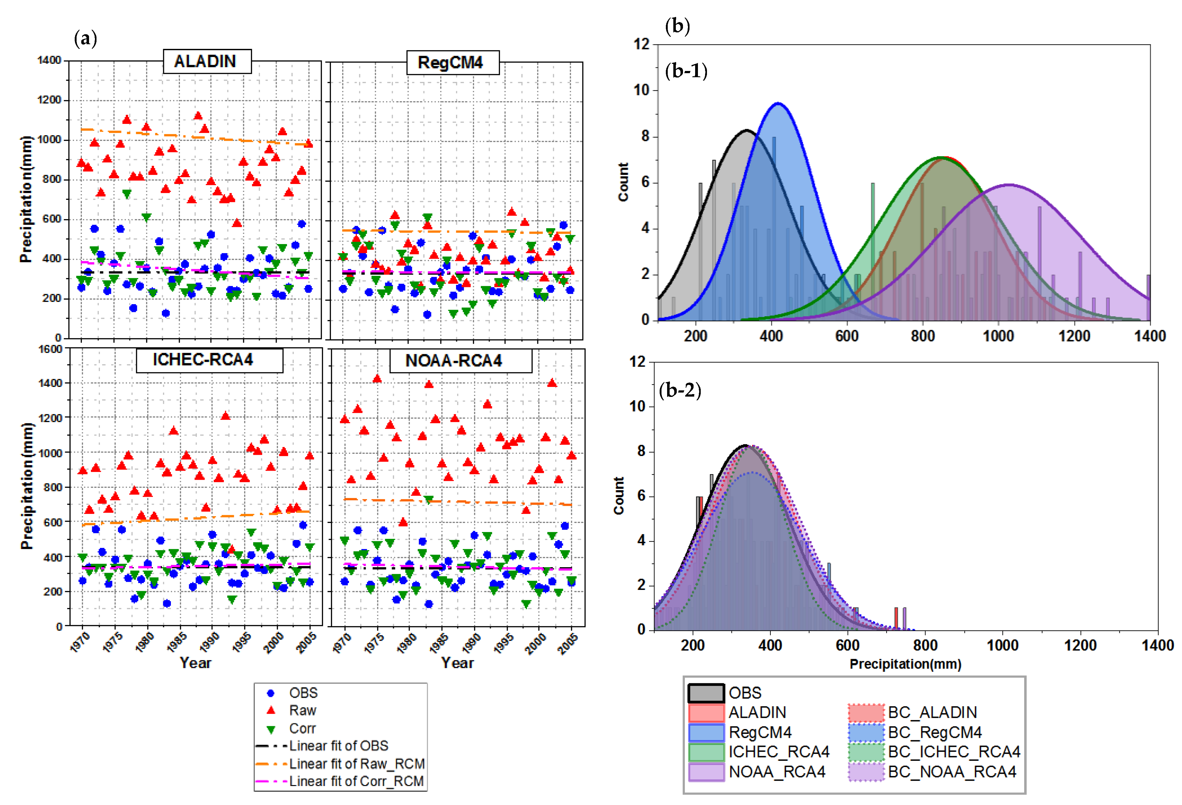
Figure 5a shows quantile–quantile (Q-Q) plots of seasonal averaged precipitation for uncorrected and corrected RCMs versus observed data for the four seasons (December, January, February (DJF); March, April, May (MAM); (JJA); September, October, November (SON)); we notice that in general, all uncorrected quantiles have more inter-model variability. Prior to bias adjustment and regarding MED-CORDEX models; the raw ALADIN outperformed the other models during the winter (DJF) season but tended to overestimate precipitation during the other seasons, particularly during the summer (JJA) when it inflated precipitation estimates significantly. Torma et al. (2020) [97] reported a similar outcome regarding this model in summer in the European Carpathian region. The uncorrected RegCM4 was the closest in estimating rainfall in all three seasons, spring (MAM), summer (JJA), and autumn (SON). As for the uncorrected MENA-CORDEX models (ICHEC-RCA4 and NOAA-RCA4), both overestimated precipitation in all seasons. After bias correction, the adjusted quantiles approach the observation. Figure 5b compares the empirical cumulative density distribution (ECDF) of observed, raw RCMs, and bias-adjusted (BC-RCMs) seasonal precipitation during the period (1970–2005) area-averaged throughout the Wadi Chemora basin. After implementing GQM bias correction, the gap between model and observation is minimized, and the corrected distributions of BC_RCMs match the observation better for all seasons, notably during the spring (MAM) season.

3.1.4. Annual Scale

Figure 6 compares the area-averaged annual precipitation of observed data, raw, and adjusted RCMs in Wadi Chemora Basin region from 1970 to 2005. Section (a) of Figure 6 (the scatter plot) shows that the annual average precipitation of corrected models approached the observed average values, which is more obvious when we look at the best fit lines that run through the scatterplot of BC RCMs, which got closer to the observed precipitation best fit line after being too far apart when the raw output of the RCMs was compared to the observations. Looking at section (b) of Figure 6, the GQM correction method also did a great job in terms of the distribution of the annual averaged precipitation, as the normal distribution of corrected RCMs nearly matched the normal distribution of observed values, and even the shape of the spread of a distribution that refers to the variability of the data improved after bias correction and became almost similar to the shape of the spread of the distribution of observed precipitation for all the RCMs.

3.2. Spatial Analysis

The spatial distributions provided by the IDW method [90,94] for the annual (Figure 7) and seasonal (Figure 8 and Figure 9) averages of precipitation for the period of (1970–2005), show that the most uncorrected RCMs overestimate precipitation over the entire study region, except for a modest underestimation of annual averaged precipitation by the RegCM4 model in the south of the study region. By examining the spatial distribution of the observed annual and seasonal averages of precipitation in the study area, we can see that the highest section of the Wadi Chemora basin in the south receives the most precipitation, particularly the southeastern region around the Ain Tinn and Foum Toub stations, and by approaching the outlet of the basin in the north (the lowest part of the basin), the precipitation hits its lowest levels. This validates the conclusions of several Algerian studies that highlighted the influence of altitude on precipitation behavior in Algeria, e.g., [102,103,104]. According to the spatial distribution of RCM’s annual and seasonal averages before correcting the biases, the MENA models ICHEC-RCA4 and NOAA-RCA4 succeeded in representing this conceptualization, which is that the low areas of the basin receive the least amount of precipitation and the high areas receive the largest amounts of precipitation. As previously stated in “Section 3.1.1”, the performance of this RCM is related to elevation [95], in contrast to the MED models ALADIN and RegCM4, which showed no behavior or relationship with altitudes.

However, after using the GQM bias correction approach, the spatial distribution of annual and seasonal precipitation averages for corrected models (BC_RCMs) largely resembles the spatial distribution of averaged observation [54].

Comparing the spatial distributions of observed average annual and seasonal precipitation and the spatial distributions of adjusted RCMs (BC_RCMs), the BC_ALADIN outperforms the rest of the models in matching the spatial distribution of annual averaged observed precipitation (Figure 7) and spatial distribution in winter (DJF) (Figure 8a), whereas BC_RegCM4 did a great job in summer (JJA) (Figure 8b). After adjusting biases, all models produced nearly identical spatial distributions of average precipitation for the autumn and spring seasons (Figure 9a,b).

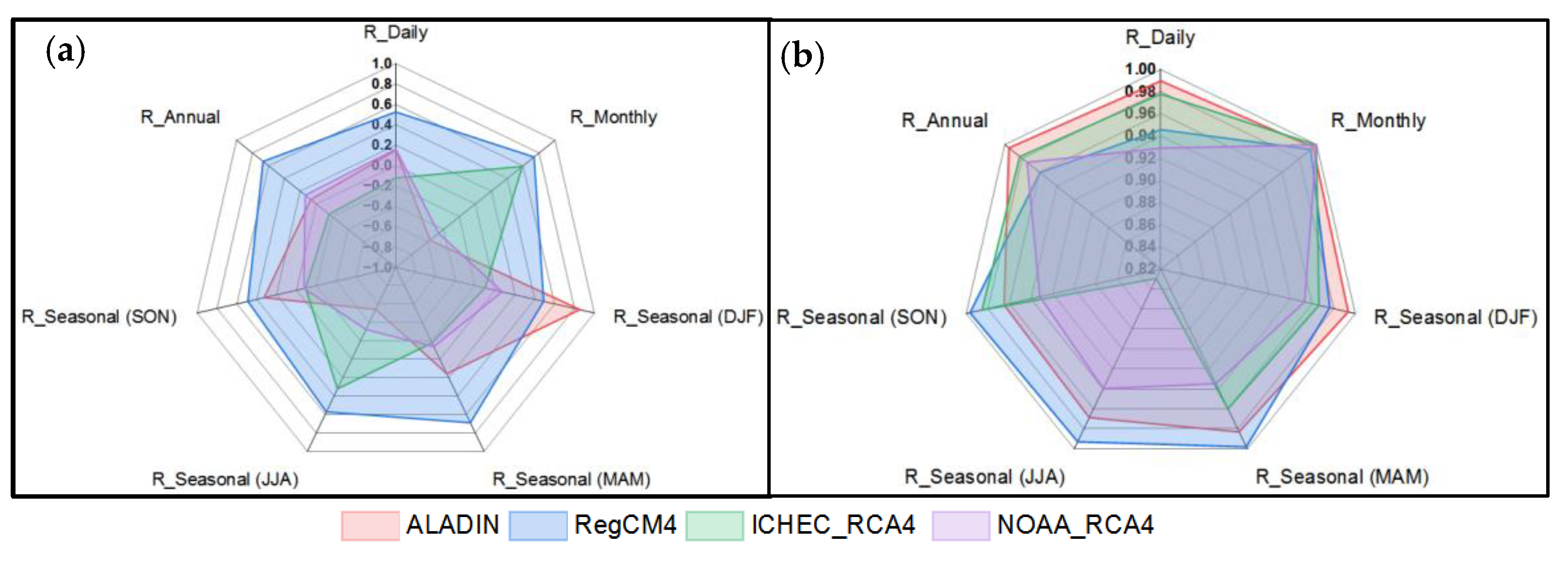
3.3. Evaluation of Bias Correction Method

The degree of statistical resemblance between the simulated and observable fields can be briefly quantified and displayed in the form of Taylor diagrams [67,84,97].

Figure 10 summarizes the performance of each RCM before and after bias correction over the Wadi Chemora basin with respect to averaged observed precipitation in different time steps (Figure 10: Daily (a), Monthly (b), Seasonal (c), and Annual (d)) for the period (1970–2005) in the form of Taylor diagrams; all RCMs simulations are depicted in Figure 10 by symbols filled with different colors. Color denotes the RCM (ALADIN in red, RegCM4 in blue, ICHEC-RCA4 in green, and NOAA-RCA4 in purple), whereas the raw and bias-corrected simulated precipitation is marked by distinct symbols.

The azimuthal position of the symbols in Figure 10 represents the correlation coefficient R between the RCM simulations and the observation, the radial distance from the reference point to each symbol represents the centered RMSE, and the distance from point 0 represents the ratio of standard deviation σ derived from the RCM simulations to the observations. Figure 10 reports the imperfection of the raw RCMs simulations and the efficiency of the GQM correction approach in improving model performance by making them close to match the reference (observation) in most time steps. Regarding the centered RMSE and standard deviation (in Figure 10) both exhibit strong evidence of bias correction on RCM precipitation fields by trending towards them to the observations.

The radar chart in Figure 11 summarizes the spatial correlation coefficients R determined using Taylor diagrams at various time steps (daily, monthly, seasonal, and annual) for each model. The raw outputs of the RegCM4 model (Figure 11a) correlated well with observations at all-time steps (R ranging from 0.49 to 0.74). While the rest of the raw RCMs simulations are characterized by very low (or even negative) and high (in case of ALADIN in (DJF) season) spatial correlation coefficients, varying between –0.56 and 0.83. The results demonstrated improvements in the spatial correlations to over 0.9 after bias correction for all RCMs at all-time steps.

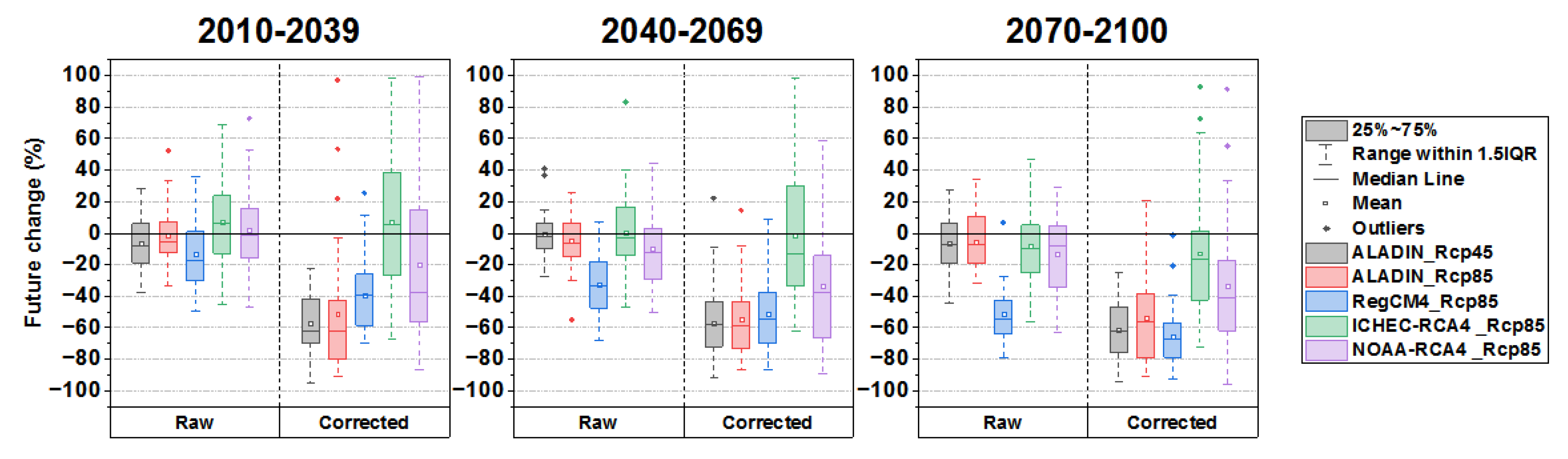
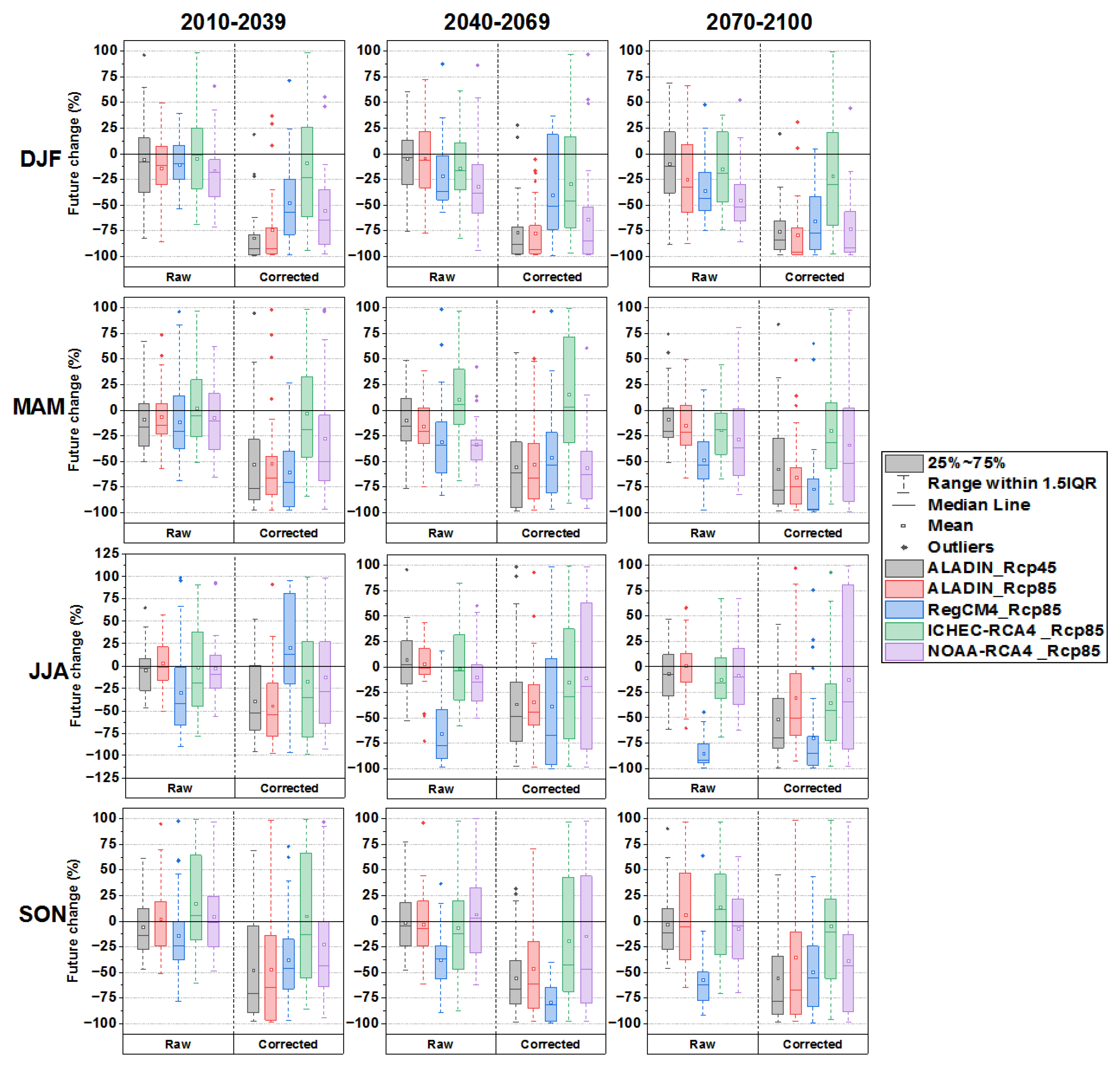
3.4. Future Projections

The GQM parametrization estimation is conducted for the model’s data in the historical period. By assuming that the GQM method is stationary, the correction algorithm and its parametrization for historical climate conditions are assumed to be valid for future conditions as well [60,85,86], so based on bias-corrected simulation outputs we projected the future precipitation [60,105]. After evaluating GQM in the historical period (1970–2005), it was used to correct the RCM projections [56,60] 2006–2100 (2006–2099 for RegCM4) forced by the Representative Concentration Pathways (RCP 4.5 and RCP8.5 for ALADIN and just RCP 8.5 for the other models).

Several studies demonstrate that precipitation in the Mediterranean and North African regions would decrease in the future under RCPs 4.5 and 8.5 [106,107,108]. This is supported by our findings in this study, in which we found that, in comparison to each model’s baseline (1970–2005) and according to the Mann–Kendall test, the future projections obtained from (RegCM4, ICHEC-RCA4, NOAA-RCA4) under RCP 8.5 have shown a significant decreasing trend, whereas raw ALADIN under RCPs 4.5 and 8.5 have shown a non-significant decreasing trend at the 5% level, and after bias adjustment this model under both RCPs (4.5 and 8.5) consistently predicts a significant future decrease in precipitation over the study region (

Table 3. Mann–Kendall trend test for future annual precipitation RCPs 4.5 and 8.5 scenarios for RCMs before and after the bias correction.

	Kendall’s Tau	p-Value	Alpha	Sen’s Slope	Trend
ALADIN_Rcp 45	−0.0863	0.144	0.05	−0.4729	Not significant
ALADIN_Rcp 85	−0.1011	0.0871	0.05	−0.5705	Not significant
RegCM4_Rcp 85	−0.5024	<0.0001	0.05	−2.1233	Significantly decreasing
ICHEC-RCA4_Rcp 85	−0.1160	0.0495	0.05	−0.9348	Significantly decreasing
NOAA-RCA4_Rcp 85	−0.1635	0.0056	0.05	−1.6848	Significantly decreasing
BC_ALADIN_Rcp 45	−0.3924	<0.0001	0.05	−1.7151	Significantly decreasing
BC_ALADIN_Rcp 85	−0.3031	<0.0001	0.05	−1.5788	Significantly decreasing
BC_RegCM4_Rcp 85	−0.4953	<0.0001	0.05	−2.1075	Significantly decreasing
BC_ICHEC-RCA4_Rcp 85	−0.1406	0.0173	0.05	−0.7195	Significantly decreasing
BC_NOAA-RCA4_Rcp 85	−0.2207	0.0002	0.05	−1.3015	Significantly decreasing

and Figure 12).

To assess future change, the raw and corrected historical period (1970–2005), were compared to the corresponding raw and bias-corrected future precipitations based on the two scenarios RCP 4.5 and RCP 8.5, for near-term (2010–2039), medium-term (2040–2069), and long-term (2070–2100). Figure 13 depicts future changes in annual average precipitation, while seasonal future changes are shown in Figure 14.

In general, before bias correction, most of the RCMs’ projections showed reductions in annual mean precipitation for all. However, for the near-term period (2010–2039), only ICHEC-RCA4 and NOAA-RCA4 under RCP 8.5 projected a slight increase (between 2% and 7% in average). After adjusting the models, all models predict an annual decrease that affects the three sub-periods reaching an average of 66% according to RegCM4 model under RCP 8.5 in the long term period (2070–2100) (Figure 13).

Figure 14 shows that prior to bias correction, the four RCMs project slight changes in future mean seasonal precipitation for the four seasons (DJF, MAM, JJA, and SON) in the near-term period (2010–2039), oscillating between slight increases and decreases, with the exception of RegCM4, which projects a 29% decrease in the JJA season. For the medium (2040–2069) and long-term (2070–2100) periods, the non-adjusted RCMs predicted a decrease in mean seasonal precipitation for the majority of seasons, notably the RegCM4 model, which predicts a massive decrease for the JJA season in the long-term period.

After the bias correction all four RCMs projected decreases in mean seasonal precipitation across the four seasons in the three sub-periods (near, medium, and long term) reaching an average of −79% autumn season (SON) according to RegCM4 model under RCP 8.5 in the medium-term period (2040–2069), with the exception of slight increases of 15% predicted by the ICHEC-RCA4 model in spring season (MAM) of the medium period (2040–2069) and 21% predicted by RegCM4 in the summer of (2010–2039) period.

4. Conclusions and Recommendation

By investigating the performances of four RCMs, ALADIN and RegCM4 from the MED CORDEX domain and ICHEC-RCA4 and NOAA-RCA4 from the MENA CORDEX domain in estimating precipitation in Wadi Chemora basin for different time steps (Daily, Monthly, Seasonal, and Annual) of the historical period 1970–2005, and the projections 2006–2100 (2006–2099 for RegCM4) forced by the Representative Concentration Pathways (RCP 4.5 and RCP8.5 for ALADIN and just RCP 8.5 for the other models) the following conclusions can be drawn:

The main findings led us to conclude that prior to bias correction, most RCMs overestimated precipitation. The GQM method worked effectively in adjusting those models for all time steps:

• The model’s resolution is not considered an influential factor in this study area, because it has been found that a model with a medium resolution of 22° (e.g., ICHEC-RCA4 from the MENA CORDEX) can outperform a model with a high resolution of 11° on occasion (e.g., RegCM4 from MED CORDEX in the daily and seasonal time steps);
• There is a relationship between the elevations and the performance of MENA-CORDEX models RCA4v1 driven by two GCMs, ICHEC-EC-EARTH and NOAA-GFDL-GFDL-ESM2M, since they performed better at lower elevations (from 1000 m to 1112 m) and poorly at higher altitudes (from 1160 m to 1650 m);
• For future projection and with respect to the corrected baseline (the historic period of 1970–2005), the adjusted RCPs of the four RCMs revealed a decreasing trend of average precipitation over the period 2006–2100 (2006–2099 for ICTP-RegCM4-3v1);
• Dividing the future time into sub-periods allowed us to see the behavior of each model individually in terms of forecasting the average precipitation in the near (2010–2039), medium (2040–2069), and long-term future (2070–2100). In summary, after adjusting the models, all of them predict a decrease that affects the four seasons of the three sub-periods, which leads to an annual decrease as well, reaching an average of 66%;
• Furthermore, our proposed approach can contribute to a reduction in precipitation prediction uncertainties and in the establishment of sustainable water resources management plans for mitigating natural disasters caused by future climate changes. We plan to extend the applicability and accessibility of the suggested method to a hydrological model, which will contribute considerably to the preparation for and adaptation to uncertain climate changes.

References

1. Maibach, E.; Myers, T.; Leiserowitz, A. Climate Scientists Need to Set the Record Straight: There Is a Scientific Consensus That Human-caused Climate Change Is Happening. Earths Future 2014, 2, 295–298. [Google Scholar] [CrossRef]
2. Harvey, B.J. Human-Caused Climate Change Is Now a Key Driver of Forest Fire Activity in the Western United States. Proc. Natl. Acad. Sci. USA 2016, 113, 11649–11650. [Google Scholar] [CrossRef] [Green Version]
3. Trenberth, K.E. Climate Change Caused by Human Activities Is Happening and It Already Has Major Consequences. J. Energy Nat. Resour. Law 2018, 36, 463–481. [Google Scholar] [CrossRef]
4. Eyring, V.; Gillett, N.P.; Achutarao, K.M.; Barimalala, R.; Barreiro Parrillo, M.; Bellouin, N.; Cassou, C.; Durack, P.J.; Kosaka, Y.; McGregor, S.; et al. Human Influence on the Climate System. In Climate Change 2021: The Physical Science Basis. Contribution of Working Group I to the Sixth Assessment Report of the Intergovernmental Panel on Climate Change; Masson-Delmotte, V., Zhai, P., Pirani, A., Connors, S.L., Péan, C., Berger, S., Caud, N., Chen, Y., Goldfarb, L., Gomis, M.I., et al., Eds.; Cambridge University Press: Cambridge, UK; New York, NY, USA, 2021; pp. 423–552. [Google Scholar] [CrossRef]
5. Shayegh, S.; Moreno-Cruz, J.; Caldeira, K. Adapting to Rates versus Amounts of Climate Change: A Case of Adaptation to Sea-Level Rise. Environ. Res. Lett. 2016, 11, 104007. [Google Scholar] [CrossRef]
6. Gasim, M.B.; Juahir, H.; Azid, A.; Kamarudin, M.K.A.; Hassan, A.R.; Hairoma, N.; Sukono, S.; Subartini, B.; Damayanti, P.P.; Supian, S. Potential of Sea Level Rise Impact on South China Sea: A Preliminary Study in Terengganu, Malaysia. J. Fundam. Appl. Sci. 2018, 10, 156–168. [Google Scholar] [CrossRef]
7. Swapna, P.; Ravichandran, M.; Nidheesh, G.; Jyoti, J.; Sandeep, N.; Deepa, J.S.; Unnikrishnan, A.S. Sea-Level Rise. In Assessment of Climate Change over the Indian Region: A Report of the Ministry of Earth Sciences (MoES), Government of India; Krishnan, R., Sanjay, J., Gnanaseelan, C., Mujumdar, M., Kulkarni, A., Chakraborty, S., Eds.; Springer: Singapore, 2020; pp. 175–189. [Google Scholar] [CrossRef]
8. Hauer, M.E.; Fussell, E.; Mueller, V.; Burkett, M.; Call, M.; Abel, K.; McLeman, R.; Wrathall, D. Sea-Level Rise and Human Migration. Nat. Rev. Earth Environ. 2020, 1, 28–39. [Google Scholar] [CrossRef] [Green Version]
9. Seneviratne, S.I.; Nicholls, N.; Easterling, D.; Goodess, C.M.; Kanae, S.; Kossin, J.; Luo, Y.; Marengo, J.; McInnes, K.; Rahimi, M.; et al. Changes in Climate Extremes and Their Impacts on the Natural Physical Environment. In Managing the Risks of Extreme Events and Disasters to Advance Climate Change Adaptation; Field, C.B., Barros, V., Stocker, T.F., Dahe, Q., Eds.; Cambridge University Press: Cambridge, UK, 2012; pp. 109–230. [Google Scholar] [CrossRef] [Green Version]
10. Peterson, T.; Heim, R.; Hirsch, R.; Kaiser, D.; Brooks, H.; Diffenbaugh, N.; Dole, R.; Giovannettone, J.; Guirguis, K.; Karl, T.; et al. Monitoring and Understanding Changes in Heat Waves, Cold Waves, Floods and Droughts in the United States: State of Knowledge. Bull. Am. Meteorol. Soc. 2013, 94, 821–834. [Google Scholar] [CrossRef]
11. Thuy Vy, D.N.; Léonard, B. Climate Variability and Extreme Weather Events in the Mediterranean Region; Université Grenoble Alpes: Grenoble, France, 2021. [Google Scholar] [CrossRef]
12. Ranasinghe, R.; Ruane, A.C.; Vautard, R.; Arnell, N.; Coppola, E.; Cruz, F.A.; Dessai, S.; Islam, A.S.; Rahimi, M.; Ruiz Carrascal, D.; et al. Climate Change Information for Regional Impact and for Risk Assessment. In Climate Change 2021: The Physical Science Basis. Contribution of Working Group I to the Sixth Assessment Report of the Intergovernmental Panel on Climate Change; Masson-Delmotte, V., Zhai, P., Pirani, A., Connors, S.L., Péan, C., Berger, S., Caud, N., Chen, Y., Goldfarb, L., Gomis, M.I., et al., Eds.; Cambridge University Press: Cambridge, UK; New York, NY, USA, 2021; pp. 1767–1926. [Google Scholar] [CrossRef]
13. Trenberth, K. Changes in Precipitation with Climate Change. Clim. Res. 2011, 47, 123–138. [Google Scholar] [CrossRef] [Green Version]
14. Giorgi, F.; Lionello, P. Climate Change Projections for the Mediterranean Region. Glob. Planet. Chang. 2008, 63, 90–104. [Google Scholar] [CrossRef]
15. Raible, C.C.; Ziv, B.; Saaroni, H.; Wild, M. Winter Synoptic-Scale Variability over the Mediterranean Basin under Future Climate Conditions as Simulated by the ECHAM5. Clim. Dyn. 2010, 35, 473–488. [Google Scholar] [CrossRef] [Green Version]
16. Piras, M.; Mascaro, G.; Deidda, R.; Vivoni, E.R. Impacts of Climate Change on Precipitation and Discharge Extremes through the Use of Statistical Downscaling Approaches in a Mediterranean Basin. Sci. Total Environ. 2016, 543, 952–964. [Google Scholar] [CrossRef]
17. Raymond, F.; Ullmann, A.; Tramblay, Y.; Drobinski, P.; Camberlin, P. Evolution of Mediterranean Extreme Dry Spells during the Wet Season under Climate Change. Reg. Environ. Chang. 2019, 19, 2339–2351. [Google Scholar] [CrossRef]
18. Tuel, A.; Eltahir, E.A.B. Why Is the Mediterranean a Climate Change Hot Spot? J. Clim. 2020, 33, 15. [Google Scholar] [CrossRef]
19. Tramblay, Y.; Koutroulis, A.; Samaniego, L.; Vicente-Serrano, S.M.; Volaire, F.; Boone, A.; Le Page, M.; Llasat, M.C.; Albergel, C.; Burak, S.; et al. Challenges for Drought Assessment in the Mediterranean Region under Future Climate Scenarios. Earth-Sci. Rev. 2020, 210, 103348. [Google Scholar] [CrossRef]
20. Bazza, M.; Kay, M.; Knutson, C. Drought Characteristics and Management in North Africa and the Near East; Food and Agriculture Organization of the United Nations (FAO): Rome, Italy, 2018; ISBN 13: 978-92-5-130683-3. [Google Scholar]
21. Ouatiki, H.; Boudhar, A.; Ouhinou, A.; Arioua, A.; Hssaisoune, M.; Bouamri, H.; Benabdelouahab, T. Trend Analysis of Rainfall and Drought over the Oum Er-Rbia River Basin in Morocco during 1970–2010. Arab. J. Geosci. 2019, 12, 128. [Google Scholar] [CrossRef]
22. Ben Abdelmalek, M.; Nouiri, I. Study of Trends and Mapping of Drought Events in Tunisia and Their Impacts on Agricultural Production. Sci. Total Environ. 2020, 734, 139311. [Google Scholar] [CrossRef]
23. Fragaszy, S.R.; Jedd, T.; Wall, N.; Knutson, C.; Fraj, M.B.; Bergaoui, K.; Svoboda, M.; Hayes, M.; McDonnell, R. Drought Monitoring in the Middle East and North Africa (MENA) Region: Participatory Engagement to Inform Early Warning Systems. Bull. Am. Meteorol. Soc. 2020, 101, E1148–E1173. [Google Scholar] [CrossRef] [Green Version]
24. Ghenim, A.N.; Megnounif, A. Ampleur de la sécheresse dans le bassin d’alimentation du barrage Meffrouche (Nord-Ouest de l’Algérie). Physio-Géo 2013, 7, 35–49. [Google Scholar] [CrossRef]
25. Meddi, H.; Meddi, M.; Assani, A.A. Study of Drought in Seven Algerian Plains. Arab. J. Sci. Eng. 2014, 39, 339–359. [Google Scholar] [CrossRef]
26. Djellouli, F.; Bouanani, A.; Baba-Hamed, K. Caractérisation de La Sécheresse et Du Comportement Hydrologique Au Niveau Du Bassin Versant de l’oued Louza (Algérie Occidentale). Tech. Sci. Méthodes 2019, 6, 23–34. [Google Scholar] [CrossRef]
27. Bendjema, L.; Baba-Hamed, K.; Bouanani, A. Characterization of the Climatic Drought Indices Application to the Mellah Catchment, North-East of Algeria. J. Water Land Dev. 2019, 43, 28–40. [Google Scholar] [CrossRef] [Green Version]
28. Bougara, H.; Hamed, K.B.; Borgemeister, C.; Tischbein, B.; Kumar, N. A Comparative Assessment of Meteorological Drought in the Tafna Basin, Northwestern Algeria. J. Water Land Dev. 2021, 78–93. [Google Scholar] [CrossRef]
29. Weart, S. The Development of General Circulation Models of Climate. Stud. Hist. Philos. Sci. Part B Stud. Hist. Philos. Mod. Phys. 2010, 41, 208–217. [Google Scholar] [CrossRef]
30. Taylor, K.E.; Stouffer, R.J.; Meehl, G.A. An Overview of CMIP5 and the Experiment Design. Bull. Am. Meteorol. Soc. 2012, 93, 485–498. [Google Scholar] [CrossRef] [Green Version]
31. Gulizia, C.; Camilloni, I. Comparative Analysis of the Ability of a Set of CMIP3 and CMIP5 Global Climate Models to Represent Precipitation in South America. Int. J. Climatol. 2015, 35, 583–595. [Google Scholar] [CrossRef]
32. PCMDI—CMIP5 Overview. Available online: https://pcmdi.llnl.gov/mips/cmip5/ (accessed on 9 March 2022).
33. Buser, C.M.; Künsch, H.R.; Weber, A. Biases and Uncertainty in Climate Projections: Uncertainty in Climate Projections. Scand. J. Stat. 2010, 37, 179–199. [Google Scholar] [CrossRef]
34. Wang, C.; Zhang, L.; Lee, S.-K.; Wu, L.; Mechoso, C.R. A Global Perspective on CMIP5 Climate Model Biases. Nat. Clim. Chang. 2014, 4, 201–205. [Google Scholar] [CrossRef]
35. Song, Y.H.; Chung, E.-S.; Shiru, M.S. Uncertainty Analysis of Monthly Precipitation in GCMs Using Multiple Bias Correction Methods under Different RCPs. Sustainability 2020, 12, 7508. [Google Scholar] [CrossRef]
36. Vrac, M.; Stein, M.L.; Hayhoe, K.; Liang, X.-Z. A General Method for Validating Statistical Downscaling Methods under Future Climate Change. Geophys. Res. Lett. 2007, 34, L18701. [Google Scholar] [CrossRef] [Green Version]
37. Benestad, R.E.; Chen, D.; Hanssen-bauer, I. Empirical-Statistical Downscaling; World Scientific Publishing Company Toh Tuck Link: Singapore, 2008; ISBN 13: 978-981-310-729-8. [Google Scholar]
38. Xue, Y.; Janjic, Z.; Dudhia, J.; Vasic, R.; De Sales, F. A Review on Regional Dynamical Downscaling in Intraseasonal to Seasonal Simulation/Prediction and Major Factors That Affect Downscaling Ability. Atmos. Res. 2014, 147–148, 68–85. [Google Scholar] [CrossRef] [Green Version]
39. Xu, Z.; Han, Y.; Yang, Z. Dynamical Downscaling of Regional Climate: A Review of Methods and Limitations. Sci. China Earth Sci. 2019, 62, 365–375. [Google Scholar] [CrossRef]
40. Adachi, S.A.; Tomita, H. Methodology of the Constraint Condition in Dynamical Downscaling for Regional Climate Evaluation: A Review. J. Geophys. Res. Atmos. 2020, 125. [Google Scholar] [CrossRef]
41. Jang, S.; Kavvas, M.L. Downscaling Global Climate Simulations to Regional Scales: Statistical Downscaling versus Dynamical Downscaling. J. Hydrol. Eng. 2015, 20, A4014006. [Google Scholar] [CrossRef]
42. Walton, D.; Berg, N.; Pierce, D.; Maurer, E.; Hall, A.; Lin, Y.-H.; Rahimi, S.; Cayan, D. Understanding Differences in California Climate Projections Produced by Dynamical and Statistical Downscaling. J. Geophys. Res. Atmos. 2020, 125, e2020JD032812. [Google Scholar] [CrossRef]
43. CORDEX | Regional Climate Model Evaluation System. Available online: https://rcmes.jpl.nasa.gov/content/cordex (accessed on 12 March 2022).
44. Noguer, M.; Jones, R.; Murphy, J. Sources of Systematic Errors in the Climatology of a Regional Climate Model over Europe. Clim. Dyn. 1998, 14, 691–712. [Google Scholar] [CrossRef]
45. Misra, V. Addressing the Issue of Systematic Errors in a Regional Climate Model. J. Clim. 2007, 20, 801–818. [Google Scholar] [CrossRef] [Green Version]
46. Ehret, U.; Zehe, E.; Wulfmeyer, V.; Warrach-Sagi, K.; Liebert, J. HESS Opinions “Should We Apply Bias Correction to Global and Regional Climate Model Data?”. Hydrol. Earth Syst. Sci. 2012, 16, 3391–3404. [Google Scholar] [CrossRef] [Green Version]
47. Sørland, S.L.; Schär, C.; Lüthi, D.; Kjellström, E. Bias Patterns and Climate Change Signals in GCM-RCM Model Chains. Environ. Res. Lett. 2018, 13, 074017. [Google Scholar] [CrossRef]
48. Dosio, A.; Paruolo, P. Bias Correction of the ENSEMBLES High-Resolution Climate Change Projections for Use by Impact Models: Evaluation on the Present Climate. J. Geophys. Res. 2011, 116, D16106. [Google Scholar] [CrossRef] [Green Version]
49. Muerth, M.J.; Gauvin St-Denis, B.; Ricard, S.; Velázquez, J.A.; Schmid, J.; Minville, M.; Caya, D.; Chaumont, D.; Ludwig, R.; Turcotte, R. On the Need for Bias Correction in Regional Climate Scenarios to Assess Climate Change Impacts on River Runoff. Hydrol. Earth Syst. Sci. 2013, 17, 1189–1204. [Google Scholar] [CrossRef] [Green Version]
50. Ruffault, J.; Martin-StPaul, N.K.; Duffet, C.; Goge, F.; Mouillot, F. Projecting Future Drought in Mediterranean Forests: Bias Correction of Climate Models Matters! Theor. Appl. Climatol. 2014, 117, 113–122. [Google Scholar] [CrossRef]
51. Johnson, F.; Sharma, A. What Are the Impacts of Bias Correction on Future Drought Projections? J. Hydrol. 2015, 525, 472–485. [Google Scholar] [CrossRef] [Green Version]
52. Sangelantoni, L.; Tomassetti, B.; Colaiuda, V.; Lombardi, A.; Verdecchia, M.; Ferretti, R.; Redaelli, G. On the Use of Original and Bias-Corrected Climate Simulations in Regional-Scale Hydrological Scenarios in the Mediterranean Basin. Atmosphere 2019, 10, 799. [Google Scholar] [CrossRef] [Green Version]
53. Ghimire, U.; Srinivasan, G.; Agarwal, A. Assessment of Rainfall Bias Correction Techniques for Improved Hydrological Simulation. Int. J. Climatol. 2019, 39, 2386–2399. [Google Scholar] [CrossRef]
54. Worku, G.; Teferi, E.; Bantider, A.; Dile, Y.T. Statistical Bias Correction of Regional Climate Model Simulations for Climate Change Projection in the Jemma Sub-Basin, Upper Blue Nile Basin of Ethiopia. Theor. Appl. Climatol. 2020, 139, 1569–1588. [Google Scholar] [CrossRef]
55. Zeroual, A.; Assani, A.A.; Meddi, H.; Bouabdelli, S.; Zeroual, S.; Alkama, R. Assessment of Projected Precipitations and Temperatures Change Signals over Algeria Based on Regional Climate Model: RCA4 Simulations. In Water Resources in Algeria—Part I; Negm, A.M., Bouderbala, A., Chenchouni, H., Barceló, D., Eds.; The Handbook of Environmental Chemistry; Springer International Publishing: Cham, Switzerland, 2020; Volume 97, pp. 135–159. [Google Scholar] [CrossRef]
56. Mami, A.; Raimonet, M.; Yebdri, D.; Sauvage, S.; Zettam, A.; Perez, J.M.S. Future Climatic and Hydrologic Changes Estimated by Bias-Adjusted Regional Climate Model Outputs of the Cordex-Africa Project: Case of the Tafna Basin (North-Western Africa). Int. J. Glob. Warm. 2021, 23, 58. [Google Scholar] [CrossRef]
57. Piani, C.; Haerter, J.O.; Coppola, E. Statistical Bias Correction for Daily Precipitation in Regional Climate Models over Europe. Theor. Appl. Climatol. 2010, 99, 187–192. [Google Scholar] [CrossRef] [Green Version]
58. Chen, J.; Brissette, F.P.; Leconte, R. Uncertainty of Downscaling Method in Quantifying the Impact of Climate Change on Hydrology. J. Hydrol. 2011, 401, 190–202. [Google Scholar] [CrossRef]
59. Themeßl, M.J.; Gobiet, A.; Heinrich, G. Empirical-Statistical Downscaling and Error Correction of Regional Climate Models and Its Impact on the Climate Change Signal. Clim. Chang. 2012, 112, 449–468. [Google Scholar] [CrossRef]
60. Teutschbein, C.; Seibert, J. Bias Correction of Regional Climate Model Simulations for Hydrological Climate-Change Impact Studies: Review and Evaluation of Different Methods. J. Hydrol. 2012, 456–457, 12–29. [Google Scholar] [CrossRef]
61. Lafon, T.; Dadson, S.; Buys, G.; Prudhomme, C. Bias Correction of Daily Precipitation Simulated by a Regional Climate Model: A Comparison of Methods: Bias Correction of Daily Precipitation Simulated by a Regional Climate Model. Int. J. Climatol. 2013, 33, 1367–1381. [Google Scholar] [CrossRef] [Green Version]
62. Chen, H.; Guo, J.; Zhang, Z.; Xu, C.-Y. Prediction of Temperature and Precipitation in Sudan and South Sudan by Using LARS-WG in Future. Theor. Appl. Climatol. 2013, 113, 363–375. [Google Scholar] [CrossRef]
63. Switanek, M.B.; Troch, P.A.; Castro, C.L.; Leuprecht, A.; Chang, H.-I.; Mukherjee, R.; Demaria, E.M.C. Scaled Distribution Mapping: A Bias Correction Method That Preserves Raw Climate Model Projected Changes. Hydrol. Earth Syst. Sci. 2017, 21, 2649–2666. [Google Scholar] [CrossRef] [Green Version]
64. Reiter, P.; Gutjahr, O.; Schefczyk, L.; Heinemann, G.; Casper, M. Does Applying Quantile Mapping to Subsamples Improve the Bias Correction of Daily Precipitation?: Does Quantile Mapping Benefit from Subsampling? Int. J. Climatol. 2018, 38, 1623–1633. [Google Scholar] [CrossRef]
65. Heo, J.-H.; Ahn, H.; Shin, J.-Y.; Kjeldsen, T.R.; Jeong, C. Probability Distributions for a Quantile Mapping Technique for a Bias Correction of Precipitation Data: A Case Study to Precipitation Data Under Climate Change. Water 2019, 11, 1475. [Google Scholar] [CrossRef] [Green Version]
66. Ayugi, B.; Tan, G.; Ruoyun, N.; Babaousmail, H.; Ojara, M.; Wido, H.; Mumo, L.; Ngoma, N.H.; Nooni, I.K.; Ongoma, V. Quantile Mapping Bias Correction on Rossby Centre Regional Climate Models for Precipitation Analysis over Kenya, East Africa. Water 2020, 12, 801. [Google Scholar] [CrossRef] [Green Version]
67. Ngai, S.T.; Tangang, F.; Juneng, L. Bias Correction of Global and Regional Simulated Daily Precipitation and Surface Mean Temperature over Southeast Asia Using Quantile Mapping Method. Glob. Planet. Chang. 2017, 149, 79–90. [Google Scholar] [CrossRef] [Green Version]
68. Zeroual, A.; Assani, A.A.; Meddi, M.; Alkama, R. Assessment of Climate Change in Algeria from 1951 to 2098 Using the Köppen–Geiger Climate Classification Scheme. Clim. Dyn. 2019, 52, 227–243. [Google Scholar] [CrossRef]
69. Taïbi, S.; Meddi, M.; Mahé, G. Seasonal Rainfall Variability in the Southern Mediterranean Border: Observations, Regional Model Simulations and Future Climate Projections. Atmósfera 2019, 32, 39–54. [Google Scholar] [CrossRef]
70. Hadour, A.; Mahé, G.; Meddi, M. Watershed Based Hydrological Evolution under Climate Change Effect: An Example from North Western Algeria. J. Hydrol. Reg. Stud. 2020, 28, 100671. [Google Scholar] [CrossRef]
71. Bouabdelli, S.; Meddi, M.; Zeroual, A.; Alkama, R. Hydrological Drought Risk Recurrence under Climate Change in the Karst Area of Northwestern Algeria. J. Water Clim. Chang. 2020, 11, 164–188. [Google Scholar] [CrossRef]
72. Lafitte, R. Structure et relief de l’Aurès (Algérie). Bull. Assoc. Géogr. Fr. 1939, 16, 34–40. [Google Scholar] [CrossRef]
73. Hassen, M.B. Etude De La Vulnerabilite A La Desertification Par Des Methodes Quantitatives Numeriques Dans Le Massif Des Aures (algerie). Ph.D. Thesis, Université de Batna 2, Fesdis, Batna, Algeria, 2009. [Google Scholar]
74. Osborn, T.J.; Hulme, M. Development of a Relationship between Station and Grid-Box Rainday Frequencies for Climate Model Evaluation. J. Clim. 1997, 10, 1885–1908. [Google Scholar] [CrossRef]
75. Bhowmik, A.K.; Costa, A.C. Representativeness Impacts on Accuracy and Precision of Climate Spatial Interpolation in Data-Scarce Regions: Data Representativeness Impacts on Climate Spatial Interpolation. Meteorol. Appl. 2015, 22, 368–377. [Google Scholar] [CrossRef]
76. Gebrechorkos, S.H.; Hülsmann, S.; Bernhofer, C. Evaluation of Multiple Climate Data Sources for Managing Environmental Resources in East Africa. Hydrol. Earth Syst. Sci. 2018, 22, 4547–4564. [Google Scholar] [CrossRef] [Green Version]
77. Caroletti, G.N.; Coscarelli, R.; Caloiero, T. Validation of Satellite, Reanalysis and RCM Data of Monthly Rainfall in Calabria (Southern Italy). Remote Sens. 2019, 11, 1625. [Google Scholar] [CrossRef] [Green Version]
78. Bhattacharya, T.; Khare, D.; Arora, M. Evaluation of Reanalysis and Global Meteorological Products in Beas River Basin of North-Western Himalaya. Environ. Syst. Res. 2020, 9, 24. [Google Scholar] [CrossRef]
79. Ayoub, A.B.; Tangang, F.; Juneng, L.; Tan, M.L.; Chung, J.X. Evaluation of Gridded Precipitation Datasets in Malaysia. Remote Sens. 2020, 12, 613. [Google Scholar] [CrossRef] [Green Version]
80. Mengistu, A.G.; Woldesenbet, T.A.; Dile, Y.T. Evaluation of the Performance of Bias-Corrected CORDEX Regional Climate Models in Reproducing Baro–Akobo Basin Climate. Theor. Appl. Climatol. 2021, 144, 751–767. [Google Scholar] [CrossRef]
81. Teutschbein, C.; Seibert, J. Regional Climate Models for Hydrological Impact Studies at the Catchment Scale: A Review of Recent Modeling Strategies: Regional Climate Models for Hydrological Impact Studies. Geogr. Compass 2010, 4, 834–860. [Google Scholar] [CrossRef] [Green Version]
82. Teng, J.; Potter, N.J.; Chiew, F.H.S.; Zhang, L.; Wang, B.; Vaze, J.; Evans, J.P. How Does Bias Correction of Regional Climate Model Precipitation Affect Modelled Runoff? Hydrol. Earth Syst. Sci. 2015, 19, 711–728. [Google Scholar] [CrossRef] [Green Version]
83. Sennikovs, J.; Bethers, U. Statistical Downscaling Method of Regional Climate Model Results for Hydrological Modelling. In Proceedings of the 18th World IMACS/MODSIM CONGRESS, Cairns, Australia, 13–17 July 2009; pp. 3962–3968. [Google Scholar]
84. Mendez, M.; Maathuis, B.; Hein-Griggs, D.; Alvarado-Gamboa, L.-F. Performance Evaluation of Bias Correction Methods for Climate Change Monthly Precipitation Projections over Costa Rica. Water 2020, 12, 482. [Google Scholar] [CrossRef] [Green Version]
85. Taye, M.T.; Alamirew, T.; Berhanu, D. Performance of Bias Correction Methods for Hydrological Impact Study in Lake Tana Sub-Basin. 2018. Available online: https://www.researchgate.net/publication/331891618 (accessed on 15 February 2021).
86. Fang, G.H.; Yang, J.; Chen, Y.N.; Zammit, C. Comparing Bias Correction Methods in Downscaling Meteorological Variables for a Hydrologic Impact Study in an Arid Area in China. Hydrol. Earth Syst. Sci. 2015, 19, 2547–2559. [Google Scholar] [CrossRef] [Green Version]
87. Chen, F.-W.; Liu, C.-W. Estimation of the Spatial Rainfall Distribution Using Inverse Distance Weighting (IDW) in the Middle of Taiwan. Paddy Water Environ. 2012, 10, 209–222. [Google Scholar] [CrossRef]
88. Keblouti, M.; Ouerdachi, L.; Boutaghane, H. Spatial Interpolation of Annual Precipitation in Annaba-Algeria—Comparison and Evaluation of Methods. Energy Procedia 2012, 18, 468–475. [Google Scholar] [CrossRef] [Green Version]
89. Wang, Y.; Yang, H.; Yang, D.; Qin, Y.; Gao, B.; Cong, Z. Spatial Interpolation of Daily Precipitation in a High Mountainous Watershed Based on Gauge Observations and a Regional Climate Model Simulation. J. Hydrometeorol. 2017, 18, 845–862. [Google Scholar] [CrossRef]
90. Demissie, T.A.; Sime, C.H. Assessment of the Performance of CORDEX Regional Climate Models in Simulating Rainfall and Air Temperature over Southwest Ethiopia. Heliyon 2021, 7, e07791. [Google Scholar] [CrossRef]
91. Chang, C.L.; Lo, S.L.; Yu, S.L. Applying Fuzzy Theory and Genetic Algorithm to Interpolate Precipitation. J. Hydrol. 2005, 314, 92–104. [Google Scholar] [CrossRef]
92. Taylor, K.E. Summarizing Multiple Aspects of Model Performance in a Single Diagram. J. Geophys. Res. Atmos. 2001, 106, 7183–7192. [Google Scholar] [CrossRef]
93. Hamed, K.H. Trend Detection in Hydrologic Data: The Mann–Kendall Trend Test under the Scaling Hypothesis. J. Hydrol. 2008, 349, 350–363. [Google Scholar] [CrossRef]
94. Worku, G.; Teferi, E.; Bantider, A.; Dile, Y.T.; Taye, M.T. Evaluation of Regional Climate Models Performance in Simulating Rainfall Climatology of Jemma Sub-Basin, Upper Blue Nile Basin, Ethiopia. Dyn. Atmos. Oceans 2018, 83, 53–63. [Google Scholar] [CrossRef]
95. Van Vooren, S.; Van Schaeybroeck, B.; Nyssen, J.; Van Ginderachter, M.; Termonia, P. Evaluation of CORDEX Rainfall in Northwest Ethiopia: Sensitivity to the Model Representation of the Orography. Int. J. Climatol. 2019, 39, 2569–2586. [Google Scholar] [CrossRef]
96. Ngai, S.T.; Juneng, L.; Tangang, F.; Chung, J.X.; Supari, S.; Salimun, E.; Cruz, F.; Ngo-Duc, T.; Phan-Van, T.; Santisirisomboon, J.; et al. Projected Mean and Extreme Precipitation Based on Bias-Corrected Simulation Outputs of CORDEX Southeast Asia. Weather Clim. Extrem. 2022, 37, 100484. [Google Scholar] [CrossRef]
97. Torma, C.Z.; Kis, A.; Pongrácz, R. Evaluation of EURO-CORDEX and Med-CORDEX Precipitation Simulations for the Carpathian Region: Bias Corrected Data and Projected Changes. Időjárás 2020, 124, 25–46. [Google Scholar] [CrossRef]
98. Park, J.-H.; Oh, S.-G.; Suh, M.-S. Impacts of Boundary Conditions on the Precipitation Simulation of RegCM4 in the CORDEX East Asia Domain: Precipitation Simulation of RegCM4. J. Geophys. Res. Atmos. 2013, 118, 1652–1667. [Google Scholar] [CrossRef]
99. Luhunga, P.; Botai, J.; Kahimba, F. Evaluation of the Performance of CORDEX Regional Climate Models in Simulating Present Climate Conditions of Tanzania. J. South. Hemisph. Earth Syst. Sci. 2016, 66, 32–54. [Google Scholar] [CrossRef]
100. Koné, B.; Diedhiou, A.; Touré, N.E.; Sylla, M.B.; Giorgi, F.; Anquetin, S.; Bamba, A.; Diawara, A.; Kobea, A.T. Sensitivity Study of the Regional Climate Model RegCM4 to Different Convective Schemes over West Africa. Earth Syst. Dyn. 2018, 9, 1261–1278. [Google Scholar] [CrossRef] [Green Version]
101. Assamnew, A.D.; Tsidu, G.M. The Performance of Regional Climate Models Driven by Various General Circulation Models in Reproducing Observed Rainfall over East Africa. Theor. Appl. Climatol. 2020, 142, 1169–1189. [Google Scholar] [CrossRef]
102. Ghenim, A.N.; Megnounif, A. Analysis of rainfall in Northwestern Algeria. Sécheresse 2013, 24, 107–114. [Google Scholar] [CrossRef]
103. Hamlaoui-Moulai, L.; Mesbah, M.; Souag-Gamane, D.; Medjerab, A. Detecting Hydro-Climatic Change Using Spatiotemporal Analysis of Rainfall Time Series in Western Algeria. Nat. Hazards 2013, 65, 1293–1311. [Google Scholar] [CrossRef]
104. Bougara, H.; Hamed, K.B.; Borgemeister, C.; Tischbein, B.; Kumar, N. Analyzing Trend and Variability of Rainfall in The Tafna Basin (Northwestern Algeria). Atmosphere 2020, 11, 347. [Google Scholar] [CrossRef] [Green Version]
105. Tramblay, Y.; Ruelland, D.; Somot, S.; Bouaicha, R.; Servat, E. High-Resolution Med-CORDEX Regional Climate Model Simulations for Hydrological Impact Studies: A First Evaluation of the ALADIN-Climate Model in Morocco. Hydrol. Earth Syst. Sci. 2013, 17, 3721–3739. [Google Scholar] [CrossRef] [Green Version]
106. Philandras, C.M.; Nastos, P.T.; Kapsomenakis, J.; Douvis, K.C.; Tselioudis, G.; Zerefos, C.S. Long Term Precipitation Trends and Variability within the Mediterranean Region. Nat. Hazards Earth Syst. Sci. 2011, 11, 3235–3250. [Google Scholar] [CrossRef] [Green Version]
107. Brouziyne, Y.; Abouabdillah, A.; Hirich, A.; Bouabid, R.; Zaaboul, R.; Benaabidate, L. Modeling Sustainable Adaptation Strategies toward a Climate-Smart Agriculture in a Mediterranean Watershed under Projected Climate Change Scenarios. Agric. Syst. 2018, 162, 154–163. [Google Scholar] [CrossRef]
108. Meddi, M.; Eslamian, S. Uncertainties in Rainfall and Water Resources in Maghreb Countries Under Climate Change. In African Handbook of Climate Change Adaptation; Oguge, N., Ayal, D., Adeleke, L., da Silva, I., Eds.; Springer International Publishing: Cham, Switzerland, 2021; pp. 1967–2003. [Google Scholar] [CrossRef]
Figure 1. Map showing (a) the study area location and the rain gauge stations distribution and (b) the hypsometric curve of the Wadi Chemora Basin.
Atmosphere 13 01876 g001
Figure 2. Grouped Half Box–Scatter plot of raw, corrected RCMs and the observational annual cycle of daily precipitation over the historical period (1970–2005) for seven rain gauges locations in Wadi Chemora Basin.
Atmosphere 13 01876 g002
Figure 3. Grouped columns shows (a) the variance of raw, corrected RCMs and observational annual cycle of daily precipitation over the historical period (1970–2005) and (b) the number of rainy days of raw, corrected RCMs, and observational monthly cycle over (1970–2005).
Atmosphere 13 01876 g003
Figure 4. Areal-averaged monthly precipitation for observed, Raw and adjusted RCMs across the Wadi Chemora Basin region for the period (1970–2005). (a) Line graph plot; (b) heatmap plot.
Atmosphere 13 01876 g004
Figure 5. Areal-averaged seasonal (DJF, MAM, JJA, SON) precipitation for observed, raw, and adjusted (BC) RCMs for the period (1970–2005). (a) The Q-Q plot; (b) ECDF distribution.
Atmosphere 13 01876 g005
Figure 6. Areal-averaged annual precipitation for observed, raw, and adjusted (BC) RCMs for the period (1970–2005). (a) Scatter plot with fitted line; (b) normal distribution histograms with curves; (b-1) before the bias correction, (b-2) after the bias correction.
Atmosphere 13 01876 g006
Figure 7. The spatial distribution of averaged annual precipitation for observed, raw, and adjusted (BC) RCMs for the period (1970–2005) in the study area.
Atmosphere 13 01876 g007
Figure 8. The spatial distribution of averaged seasonal precipitation for observed, raw, and adjusted (BC) RCMs for the period (1970–2005) in the study area (a) for winter (DJF) and (b) for summer (JJA).
Atmosphere 13 01876 g008
Figure 9. As in Figure 7 but for (a) spring (MAM) and (b) autumn (SON)).
Atmosphere 13 01876 g009
Figure 10. Taylor diagrams of simulated precipitation (Raw and corrected RCMs) referencing to the averaged observed precipitation in different time steps (a) Daily (b) Monthly, (c) Seasonal, and (d) Annual.
Atmosphere 13 01876 g010
Figure 11. Radar charts of spatial correlation coefficients R in different time steps. (a) Raw RCMs; (b) corrected RCMs.
Atmosphere 13 01876 g011
Figure 12. Annual precipitation predicted by RCP 4.5 and RCP 8.5 with trends for predicted raw and corrected RCMs.
Atmosphere 13 01876 g012
Figure 13. Relative changes of annual average precipitation for 2010–2039, 2040–2069, and 2070–2100 (2070–2099 for RegCM4) with respect to 1970–2005. Changes are given in %.
Atmosphere 13 01876 g013
Figure 14. Future changes of seasonal average precipitation for 2010–2039, 2040–2069, and 2070–2100 (2070–2099 for ICTP-RegCM4-3v1) with respect to 1970–2005. Changes are in %.
Atmosphere 13 01876 g014