Article

Solar Signature in Climate Indices

Institute of Geodynamics, Romanian Academy, R-020032 Bucharest, Romania
*
Author to whom correspondence should be addressed.
Atmosphere 2022, 13(11), 1898; https://doi.org/10.3390/atmos13111898
Submission received: 8 October 2022 / Revised: 6 November 2022 / Accepted: 10 November 2022 / Published: 13 November 2022
(This article belongs to the Section Climatology)

Abstract

:
The influence of solar/geomagnetic activity on climate variables still remains a fully unclarified problem, although many scientific efforts have been made to better understand it. In order to bring more information to this open problem, in the present study, we analyze the connection between solar/geomagnetic activity (predictors) and climate variables (predictands) by applying elements from information theory and wavelet transform analysis. The solar activity was highlighted by the Wolf number and geomagnetic activity was quantified by the aa index. For the climate variables, we considered seven Climate Indices (CIs) that influence atmospheric circulation on regional or global scales, such as the Greenland-Balkan Oscillation Index (GBOI), North Atlantic Oscillation Index (NAOI), Arctic Oscillation (AO), Atlantic Multidecadal Oscillation (AMO), Southern Oscillation Index (SOI), Bivariate ENSO Timeseries (BEST) and Trans-Niño Index (TNI). By using the difference between synergy and redundancy, a few cases were found where the two predictors can be considered together for CIs’ estimation. Coherence analysis through the wavelet transform for three variables, both through multiple and partial analysis, provides the time intervals and bands of periods, where the two considered predictors can be used together or separately. The results differ depending on the predictand, the season and the considered lags. Significant information is brought out by using the two predictors together, namely the summer season, for GBOI and NAOI, when the predictors were taken 2 years before, and the winter season, as AMO responds to the variations of both solar and geomagnetic activity after 4 years.

1. Introduction

The sun is the fundamental source of energy that drives our climate system. Therefore, it can be postulated that, indubitably, solar variability is an important external source of natural climate variability. The atmosphere exhibits a number of characteristic modes of variability that are important in determining the local climate in different regions [1,2]. Many works include descriptions of some of them, as they can influence how the impact of solar variability is experienced on climate.
Numerous attempts have been made to find the connection between solar activity and terrestrial phenomena, depending on the means and stages of knowledge [1,3,4,5,6,7,8,9,10] and resulting in some disputes [11,12,13]. Solar activity has been found to be correlated with climate during the 20th century; more precisely the geomagnetic trend, in general, correlates with the evolution of the global temperature, except in the last decade [14,15,16].
Towards the second half of the most recent century, investigations suggested that the solar energy signal is an order of magnitude smaller than the atmospheric energy capable of shaping the movements of the real atmosphere [17,18,19,20].
Even nowadays, for example, such a conclusion is reached that the direct impact of sunspots on Earth’s temperature anomaly is very weak, almost minimal, but can be indirect [12,13]. The cause may be due to the inadequate analysis method for unraveling such complex connections. The direct influence of solar activity is so distorted that the Sun seems to act and chaotically influence the climate at the level of the earth’s surface.
An important factor in modulating possible solar effects on the atmosphere [8,21,22,23,24] is the Quasi-Biennial Oscillation (QBO), although the QBO has quasi-regular variations. At the stratospheric level of 30 hPa, temperature data are found to be strongly correlated with sunspot activity. On the other hand, at the level of the earth’s surface, the correlations between solar activity and air temperature are inexplicably small, as mentioned by other authors [2,11,12,25,26]. However, there are several investigations that have found significant correlations between solar activity and air temperature on the earth’s surface, especially before the 1970s (Friis-Christensen and Lassen, 1991; Lean et al., 1995; Haigh, 2003) [27,28,29]. In paper [30], Lockwood (2012) points out that if the increase in temperature due to solar activity is difficult to determine on a global scale, then such work can be performed on a regional scale by neglecting certain factors, such as greenhouse effects, and explaining the physical mechanisms. These mechanisms mainly refer to the high solar-atmosphere interaction through the so-called “top-down” mechanism.
Saltzman [31] invokes the nonlinearities in the real climate system that are “mutilated” due to linearizations produced by idealized modeling. The effects of these linearizations are reflected in multiple non-concordant forms of the climate system with those of the considered external causal factor.
Although nowadays there is almost unanimous recognition of the signature of solar activity in the earth’s climate [32,33,34], the natural climate hazard of the current period seems uncontrollable, and the range of extreme events is increasing in amplitude and frequency. The evolution of hazardous phenomena on Earth is closely related to “typical climate indices”.
In the comprehensive knowledge of these relationships, significant progress has been made both in the accumulation of long series of data (from reconstructions and reanalysis) [35] and investigative methods, as well as in the organizational framework at a more sustained international level. Thus, the Intergovernmental Panel on Climate Change’s Sixth Assessment Report (IPCC AR6) [36] emphasized both the dangerous evolution of future climate changes and the complexity of their knowledge. Deterministic models still cannot bring a major contribution as they are still limited and for now do not include methods that can discriminate between external and internal causes of climate change. As stated in IPCC AR6, the direction of causality is not clear.
Statistical methods can somehow provide an increased contribution to unlocking the complexity of the Sun–climate impact, especially regarding the non-deterministic component. Of course, the direct impact of solar activity on climate variability is difficult to outline, due to the complex processes that take place in the Sun–Earth environment, taking into consideration the complexity of their climate system. Recently, Chapman et al. [37] warned that extremely dangerous events can occur for human activity in certain situations where the geophysical environment is affected by solar activity. Thus, the response of the geophysical environment depends on multiple structures of the plasma emitted by the solar corona in its interaction with the earth’s magnetosphere.
As recently shown by Katsavrias et al. [38], solar-terrestrial coupling is achieved through the geomagnetic activity, which can be considered a precursor in the appearance of various geophysical phenomena. A correlation with a high statistical significance between certain atmospheric variables and the geomagnetic field was found by Mawad et al. [39]. This correlation is weaker on the earth’s surface and gradually increases towards the upper layers of the atmosphere.
Regarding the approach method, the prediction, “the little wave with the big future” by Addison [40] has proven to be an excellent tool in today’s investigation for understanding the interactions of phenomena at different spatio-temporal scales.
In this study, robust investigation procedures (information theory and wavelet transform) are applied, which could shed some light on the assessment of the impact of the most important natural external factor (solar/geomagnetic activity, described by the Wolf number/aa geomagnetic index) on climate evolution through “typical climate indices” to quantify nonlinear interactions and even with establish a causal chain.
Stenseth et al. [41] in their analysis specify the advantages of the application of climate indices. They by definition reduce complex space and time variability into the simple measures, which helps to appreciate the global nature of climate systems, and provide statistically tractable climate factors.
If the direct link between the main climate indices and hydro-climatic events, especially the dangerous ones, have been widely debated [42,43,44,45,46], the modification of these indices depending on the external factor was described in several works [47,48,49]. There are also a few works that investigate the link between solar/geomagnetic activity and local or regional climate variability by means of typical climate indices. Such works reported different results; for example, some found that signatures of sunspot numbers in dependent El Niño–Southern Oscillation (ENSO) variations is strong, as is shown in Hassan et al. [8] and the linear type (Markov chain). However, Nuzhdina [50] finds that cyclic dynamics of ENSO phenomena are due to solar activity and geomagnetic variations. Interesting conclusions were reached by Fu et al. [51] by which solar activity affects El Niño first, and subsequently, this influence is transferred by El Niño to the annual mean streamflow. Dobrica et al. [47] found that on multi-decadal timescales, solar variability affects firstly the Atlantic Multi-decadal Oscillation and then the hydroclimatic regime. Furthermore, Kodera et al. [24] found that solar modulation of the ENSO cycle is manifested mainly in the western extent of the Walker cell and links to the behavior of Indian Ocean monsoons.
In the present study, we set out to see through the external solar/geomagnetic factors, considered as predictors, what happens to the main climate indices considered predictands. These indices can describe atmospheric processes or ocean-atmosphere interactions, which in turn can be the precursors of hydro-climatic processes at the regional/local scale. There are different climatic indices suitable for different areas of the earth that influence atmospheric circulation. For certain climate indices such as ENSO, several variants have been developed. It is worth mentioning two of the variants: Multivariates ENSO Index (MEI) Wolter and Timlin [52], and Bivariate ENSO Timeseries (BEST) index, first described by Smith and Sardeshmukh [53]. The latter is analyzed in the present study.
First of all, the investigation in the present study is a contribution to the assessment of the sun/climate link by applying the two types of linear and non-linear relationships through typical climate indices. To outline the non-linear links, we apply information theory, which is now often used successfully in the sun/climate relationship as well [54,55,56,57,58,59].
Secondly, the synchronicity, at various periodicities, between solar/geomagnetic (Wolf/aa) indices and climate indices, is taken into consideration by using wavelet coherence.
Lorenzo-Lacruz et al. [60] successfully uses the wavelet tools to measure the coherence of two series in a time-frequency space. Because of the power of filtering and detection of different wavelet transforms, it finds specific links between atmospheric circulation quantified by atmospheric indices such as NAO and the discharge of most rivers in central and western Europe.
Special attention is given to the investigation by means of wavelet which assumes the validity of the principle of superposition even in the case of non-linear links [61,62], as is the case with most terrestrial phenomena under solar/geomagnetic impact [38,51,63,64,65,66,67]. Multiple advantages of using the wavelet, especially in detailing the information, in the analysis of time series can be found in [38,68,69,70,71,72].
It is important to underline the fact that the existing non-linear links between phenomena, approximated by linear methods, leads to a mutilation of reality and inconsistent results. However, even when there are proven linear links, it is not worth conducting an expensive investigation through sophisticated non-linear mathematical procedures. That is why it is good to test a priori if the links in question are non-linear or not.
In Hood et al. [73], robust investigations are made to explain the mechanism of the solar impact on the terrestrial climate modulated by the set of climatic indices, using both observations and simulations of general circulation models (GCM).
The present study can be a support in future investigations regarding the nature of the sun–climate relationship and details the time-frequency domain of the links obtained from the analysis of observations from the 20th century.
The paper is organized as follows: Section 2 begins with the description of the seven climate indices, associated with different modes of climate variability used in the present study, as well as the two indicators that quantify solar activity (Wolf number) and the geomagnetic activity (aa geomagnetic index) (2.1). The methods applied to find the nature of the link between the two external indicators and climate indices, as well as details regarding these relationships are given in subsection (2.2). The results and discussions are presented in Section 3. In this section, we first present and discuss the results obtained by applying the non-linear correlations between solar/geomagnetic activity indices, which are considered separately, and CIs, with lags from 0 to 5 years. The influence of the two external indices considered together, on the CIs, is also analyzed in order to highlight both the synergistic contribution and the induced redundancy. Further, in Section 3, we discuss the results obtained by multiple wavelet coherence (mwc) and partial wavelet coherence (pwc) applied for tree variables, which are two predictors and one predictand as one of the seven climate indices. In Section 4, the conclusions and future directions of investigation that emerged from this study are presented.

2. Data and Methods

2.1. Data

The datasets used in this study consist of variables that characterize terrestrial climate, climate indices, on one hand, and solar/geomagnetic indices used to describe solar/geomagnetic activity as natural external factors for the climate system, on the other hand.
The considered climate indices are: Greenland-Balkan Oscillation Index (GBOI) [74], North Atlantic Oscillation Index (NAOI) (Hurrell [75]), Arctic Oscillation (AO) (Thompson and Wallace [76]), Atlantic Multidecadal Oscillation (AMO) (Enfield et al. [77]), Southern Oscillation Index (SOI) (Ropelewski and Jones [78]), Bivariate ENSO Timeseries (BEST) (Smith and Sardeshmukh [53]) and Trans-Niño Index (TNI) (Trenberth and Stepaniak, [79]). It should be mentioned that for some of the climate indices that refer to AO, AMO and BEST, we did not add index (I) for abbreviations.
The first two indices, Greenland-Balkan Oscillation index (GBOI) and North Atlantic Oscillation index (NAOI), have been frequently used in our previous investigations [65,66,80,81,82]. The NAO index, or the difference in the normalized sea level pressure (SLP) between Lisbon (Portugal) and Stykkisholmur (Iceland), was downloaded from http://www.ldeo.columbia.edu/res/pi/NAO/ (accessed on 7 January 2001). The GBO index, which was introduced by Mares et al. [74], reflects the baric contrast between the Balkan and the Greenland zones and it was calculated as the difference in normalized SLP at Nuuk and Novi Sad. This GBOI was analyzed in several investigations [65,66,74,82] in which the significant contribution of this climatic index to the climate in the south-eastern part of Europe was demonstrated. The data for the other five indices, AO, AMO, BEST, SOI, and, TNI, were extracted from https://psl.noaa.gov/data/climateindices/list/ (accessed on 1 October 2022). Among the lesser known indicies, the BEST index was used (https://psl.noaa.gov/data/correlation/censo.long.data, accessed on 1 October 2022), which was designed to provide a long time period ENSO index for research purposes (Smith and Sardeshmukh, 2000) [53].
Regarding the TNI, which is also less accessed in climate research, details can be found in Trenberth and Stepaniak [79] and at https://psl.noaa.gov/gcos_wgsp/Timeseries/TNI/ (accessed on 1 July 2015).
External predictors include the Wolf sunspot number and the aa geomagnetic index. Details and data might be found at http://www.sidc.be/silso/datafiles (accessed on 11 November 2016), and at http://isgi.unistra.fr/indices_aa.php (accessed on 1 October 2022), respectively.
The Wolf sunspot number was abbreviated in the present study only by Wolf.
The analysis was performed for each season separately and for the time interval 1901–2000, simultaneously and with lags, from 1 to 5 years after the occurrence of solar/geomagnetic events. The analysis only for the 20th century and for seasonal averages was considered in this study to compare some of the results with those obtained by the authors in their previous investigations (Mares et al. [66,81,82]), where only 2 of the 7 climate indices were analyzed. It is possible that a monthly analysis will provide more detailed information regarding the solar activity signal. After analyzing the monthly rainfall values from several areas of Africa, interesting results were obtained in the paper (Lüdecke et al. [83]), in which it was found that both solar activity and the 5 climate indices used by the authors have a significant signal on African rainfall. For Europe, Laurenz et al. [84] obtained detailed results regarding the solar activity signal quantified by the number of sunspots on monthly precipitation in 39 countries.

2.2. Methods

It is generally known that the influence of solar activity on terrestrial variables is non-linear and non-stationary; therefore, in the present study, we applied methods from information theory and the wavelet transform. Thus, to highlight the degree of non-linearity, we first compared the linear and non-linear relationships between the solar/geomagnetic activity and the seven climate indices. The linear relationships were obtained by linear (Pearson correlation coefficient) and non-linear correlations. The non-linear correlation coefficient (NLR) was calculated according to the following equation:
NLR = [ 1 exp ( 2 M I ) ]
where MI is Mutual Information, which indicates the amount of information shared between the two time series.
The NLR variation range is the same as of the linear correlation coefficient but has the advantage of ignoring the statistical distribution of the analyzed variables or the nature of their relationship. Several studies detailed the performance of this nonlinear measurement in comparison with classical linear correlation (e.g., Khan et al. [85], Vu et al. [55]).
For the confidence level (CL) in the case of the Pearson correlation coefficient, specific tables were used, corresponding to series of length or 100 values (1901–2000) performed in the present study. Mares et al. [82] give details on how to obtain confidence levels in the case of NLR, according to Steuer et al. [86] and Theiler et al. [87].
Since in the present study we aimed to analyze both the influence of solar and geomagnetic activities on climate indices separately, and the influence of the two indicators considered predictors for each of the seven analyzed climate indices simultaneously, it is also necessary to estimate the difference between synergy and redundancy.
According to Timme et al. [88], in the case of the three variables, a performance analysis of predictors’ contribution (X1,X2) to predictand (Y), and also by reducing the redundancy produced by predictors, is achieved by simultaneous analysis of synergy and redundancy (Equation (2)).
S-R = Synergy (Y; X1,X2) − Redundancy (Y; X1,X2)
S R = M I ( X 1 , X 2 ; Y ) M I ( X 1 , Y ) M I ( X 2 , Y )
A negative value implies that the redundant contribution is greater in magnitude than the synergetic contribution.
We can also estimate a measure of the total correlation (TC) between all variables by means of the equation:
TC = M I ( X 1 ; X 2 ) + M I ( X 1 , X 2 ; Y )
As shown in Tary et al. [69], the problem of signal resolution in the time-frequency domain of the nonstationary processes can be solved using wavelet analysis.
A review of spectral methods and wavelet analysis, with applications for climatic time series, are widely described in Ghil et al. [70]. Si [71] reviewed the methodologies of spectral and wavelet analyses, particularly the statistical tests of spectra and coherency.
Wavelet transform is a universal mathematical method that works with non-stationary time series and detects when significant periods and their changes take place [72]. A review of wavelets in geoscience and in particular the study of correlations between solar activity and variables in the field of hydrology is given in Labat [63] and Fu et al. [51]. An interesting and extensive review of the wavelet method applied to obtain the different periodicities of the parameters that characterize the solar/geomagnetic activity can be found in the recent work by Katsavrias et al. [38].
In the present investigation, as in cases where high redundancy is present, we cannot use the two predictors together to obtain significant information for the predictand, so we attempted to determine which details in the time–frequency domain are provided by partial wavelet coherence (pwc).
As shown by Mihanović et al. [89], nonstationary wavelet analysis (Torrence and Compo) [90] was applied to obtain more detailed information on the time–frequency domain. In general, it is possible to analyze the time series according to a specific time scale using wavelets. Cross-wavelet transform (XWT) and wavelet coherence (WTC) are particularly appropriate when analyzing the relationship between two time series, with one considered as the input (predictor) and the other one as the output (predictand).
Sreedevi et al. [91] show that because there is an interaction between the variables considered as predictors, a bivariate relationship can be clearly explained only by untangling the role of other contributory variables. This can be carried out by including only one predictand and one predictor in the pwc analysis and by excluding the effect of the other predictor variables. The pwc method was suggested by Mihanović et al. [89] and then used in many studies, but in many of these studies, only two predictors were used, of which only the effect of one of the predictors was excluded.
In this study, the results obtained from wavelet coherence for three variables are presented. The three variables are the two predictors, the Wolf number and the aa geomagnetic index, and the predictand is one of the analyzed climate indices.
The details for several variables can be found in the work of Hu and Si, who generalize the partial coherence between the predictand and a set of predictors greater than three. Gu et al. [92] showed that Hu and Si [93] improved partial wavelet coherence to effectively reveal the scale-dependent coherence, periodic characteristics and lag relationship of two variables while avoiding the impacts of the other variables. Their improved partial wavelet coherence method has been successfully used in meteorology (Zhou et al. [94]) and economics (Firouzi and Wang [95]) by untangling the scale-specific and localized relationships after excluding the effects of the other variables. In other words, pwc is appropriate for finding the partial correlation between response (predictand) variable Y and the set of predictor variables X after eliminating the influence of the set of predictor variables Z.
Regarding the multiple wavelet coherence (mwc) developed by Hu and Si [96], the authors of this study applied it to find multiple coherence between different large-scale climate indices and the Danube discharge and between climate indices and indicators of solar/geomagnetic variability [65,66,67,82].
Confidence levels for multiple and partial coherence squared were calculated using the Monte Carlo method (Grinsted et al.; Maraun et al.; Jevrejeva et al.; Torrence and Webster) [97,98,99,100].

3. Results and Discussion

As was mentioned in the data section, to investigate the connection between solar/geomagnetic activity and climate indices, linear and non-linear approaches between predictors and predictands have been applied on each season with a lag from 0 to 5 years. First, we will present and analyze the results obtained by comparing the NLR correlation coefficients with those obtained by classical Pearson correlations (|R|). Therefore, the linear and non-linear correlation coefficients between the Wolf number/aa geomagnetic index and climate indices for each individual season and with lag from 0 to 5 years are presented by comparison in Figure 1. It should be mentioned that inside all Figures, aa is written in capital letters, meaning AA.
A first observation that can be noted is that in almost all cases, the values of NLR are higher than those of |R|. These results indicate that the links between the indicators for the solar/geomagnetic activity and climate variables are non-linear, as it was also shown by Vu et al. [55] and Zaidan et al. [101].
Taking into account what was mentioned in the previous section, regarding statistical significance, we found that the NLR must be > 0.4 and |R| > 0.2 at a confidence level (CL) of 95%. If we refer to a CL of at least 90%, NLR > 0.3 and |R| > 0.16.
In the following section, the results shown in Figure 1, in which CL > 95%, will be discussed. For the spring season, solar activity has a significant contribution on AMO at a lag of 5 years and on BEST at a lag of 2 years. Regarding the aa contribution on analyzed indices, there is no case with a CL > 95% for NLR, but we can mention two cases in which |R| has a CL > 95%, namely for AO and AMO at lag of 5 years.
The non-linear relationship of climate indices with solar activity in the summer season does not highlight any case with CL > 95%, but the situation of AO can be mentioned, for which the linear correlation has a CL > 95% at delays of 4 and 5 years, compared to the Wolf number. In relation to aa, for the AO variable, an NLR with CL > 95% for a lag of 2 years, and with a CL ≈ 95% at lag of 4 years is clearly observed. Furthermore, it should be emphasized that for this climate index (AO), there is a linear relationship with aa, both simultaneously and at lag 1, because |R| > NLR and R has a CL > 95%.
During the autumn season, for the relationship with the Wolf number, there are three cases when NLR has significance higher than 95%, namely, AO at a lag of 5 years, AMO at a lag of 4 years and TNI at a lag of 5 years. For correlations with aa, there is only one situation for which a relationship with the Wolf number was found, which was at AMO for a lag of 4 years.
In the winter season, the signal of solar activity on the TNI at the 5-year lag is highlighted, and that of aa on the AMO climate index simultaneously at the 1 and 4-year lags as well.
The results obtained from testing the influence of each predictor separately on the climate indices have not been presented until now.
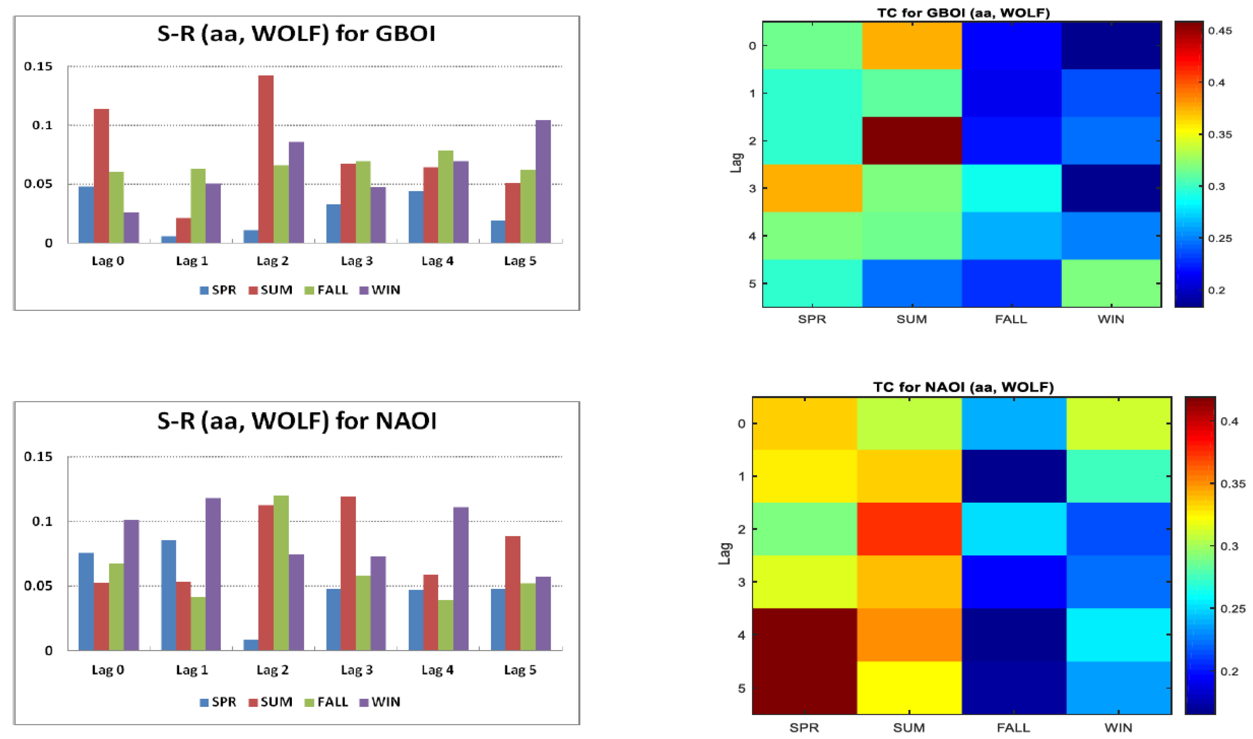
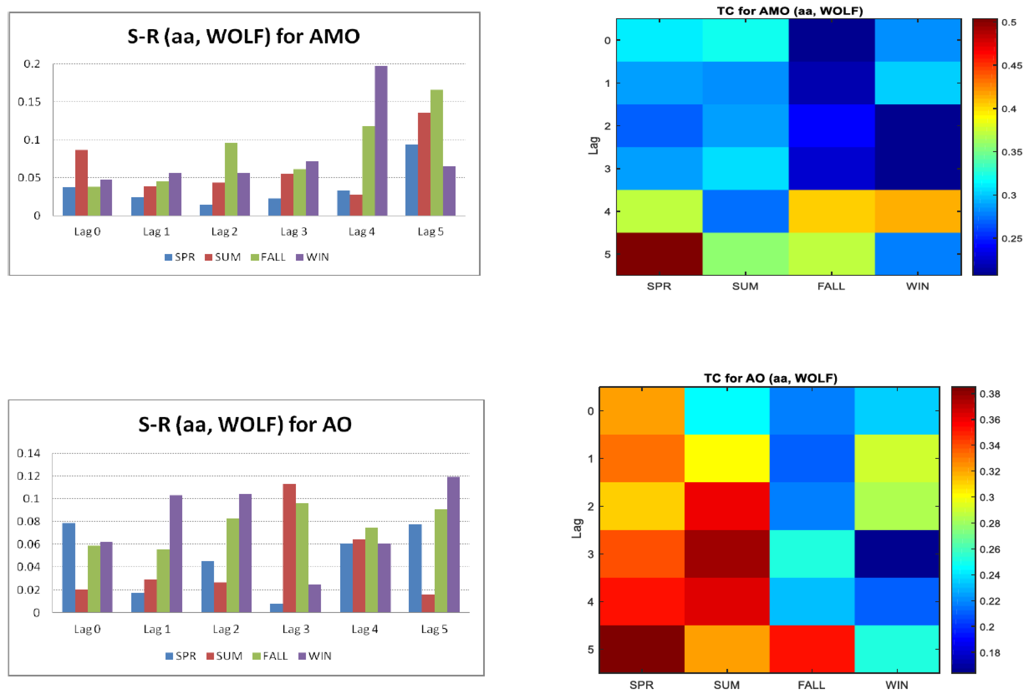
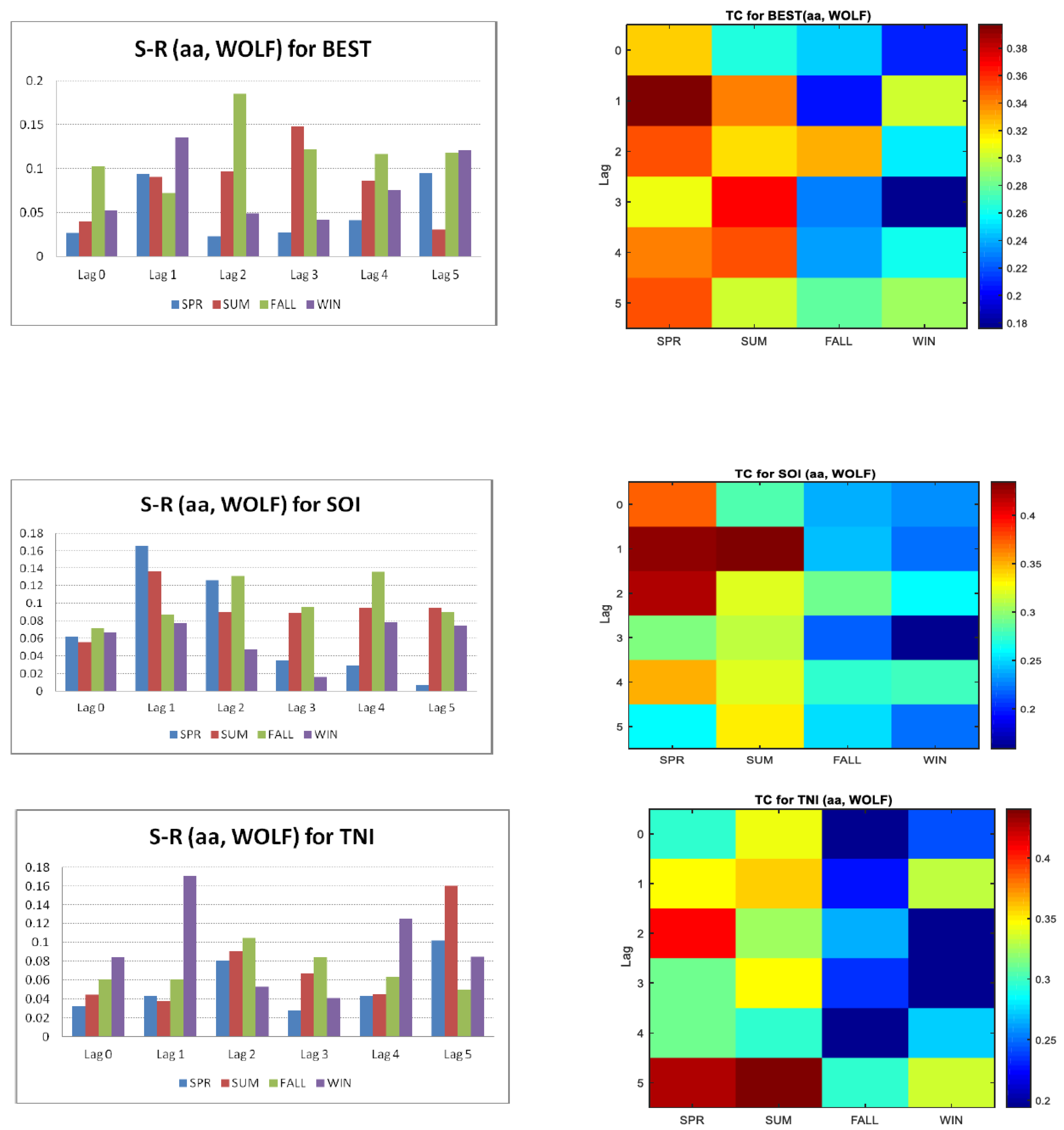
In the following section, we will discuss the results obtained by considering the influence of the two predictors, simultaneously, on each of the climate indices. We achieved this by calculating the difference between synergy and redundancy and the total correlation in accordance with relations (2) and (3). The results for each of the seven climate indices are shown in Figure 2. As in the case of individual correlations, here too we considered lags from 0 to 5 years between predictors and predictand. The results differ depending on the season and the predictand variable.
For the first climate index considered in the present study, GBOI, the highest values of S-R accompanied by high TC are during the summer at a lag of 2 years. Regarding the NAOI, the analysis of both S-R and TC values indicates that the influence of two sources on NAOI is during the summer at lags of 2 and 3 years. For AMO, the R-S value at lag 4 in winter differs from the other values and because of the relatively high TC associated with it, we conclude that both the solar and geomagnetic indices can be considered together to be significant predictors. Regarding AO, for summer with a lag of 3 years, the two predictors can be considered together. For BEST, during the fall with a lag of 2 years, the two predictors bring together their contribution to the variability of this climate index. For SOI, we can consider that both in the spring and summer seasons, the two predictors, taken with a lag of one year before, can be considered significant predictors. Taking into account both the R-S and TC values, for TNI, during the summer, after five years, the two predictors considered together can influence the behavior of this index. At this stage, it should be mentioned that the appearance of high linear/non-linear correlations between solar variability and climate with certain lags might not be unexpected, keeping in mind the complexity and non-linearity of climate systems and of their external and internal forcings. Various periodicities in solar variability indices and climate indices, for instance, could result in such lags. The physical mechanisms that are behind these lags are beyond the scope of this study. However, an explanation of the physical mechanism of correlations with certain lags between solar activity and climate variables can be found in certain studies (Gray et al. [16]; Drews et al. [49]; Scaife et al. [102]; Thiéblemont et al. [103]; Chen et al. [104]).
Further, by applying the wavelet analysis for multiple variables, the information provided by R-S is detailed. In the following section, we will present some results obtained by mwc and pwc in cases where the values of R-S are small compared to the cases where these values are high.
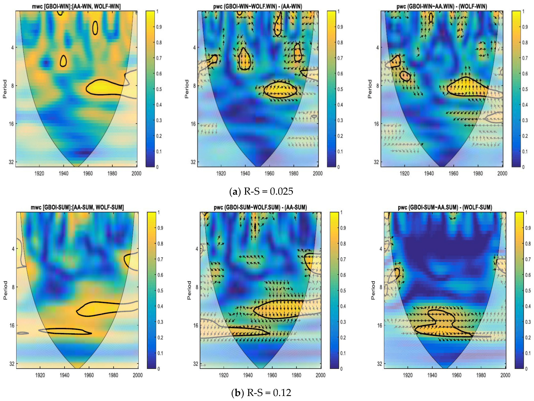
To begin with, we will discuss three results that refer to the cases where both predictors and predictand are considered simultaneous, that is lag = 0. Thus, Figure 3a shows the winter situation for GBOI and the two predictors with a small R-S (0.025) according to Figure 2. In the first panel of Figure 3a, the mwc between GBOI in winter and aa and Wolf number is presented. In the second panel, the pwc between GBOI and Wolf, eliminating the influence of aa, and in the third panel is the pwc between GBOI and aa, excluding the influence of solar index are represented. Figure 3b shows the same values, but for GBOI during summer, the season for which at lag = 0 and R-S has the highest value, i.e., 0.12. In the first case (Figure 3a), it can be seen that both the common coherence of GBOI with the two indices (predictors) and the coherence with each of the predictors, by excluding the other, are low, excluding the years 1960–1980, whereas for periods of approximately 10–11 years, significant coherences can be observed. Regarding Figure 3b with predictors, which can be considered non-redundant, their consideration together is possible for the entire considered interval (1901–2000), but especially for the intervals in the cone of influence. Thus, for the intervals between the years 1930–1980, there is a common coherence corresponding to the cyclicity between 10 and 22 years, as highlighted by mwc (left panel in Figure 3b). From the representation of the two pwc, it can be seen how the two predictors complement each other. For example, for the interval 1940–1960, for periods of approximately 16 years, aa brings a significant contribution to the coherence with GBOI. It can be seen that at pwc the phase angles differ in the case when we retain the Wolf number and eliminate aa, in comparison with the case when we retain aa and eliminate solar activity. This difference in the arrows indicating the phase is due to the fact that there is a certain time interval between the solar activity quantified by the sunspots number and the geomagnetic activity represented by aa. Details regarding the relationship between the number of sunspots and aa, of some common cyclicities, as well as the mechanisms that determine them over certain time intervals, are given in the publications (Demetrescu and Dobrica; Du) [105,106].
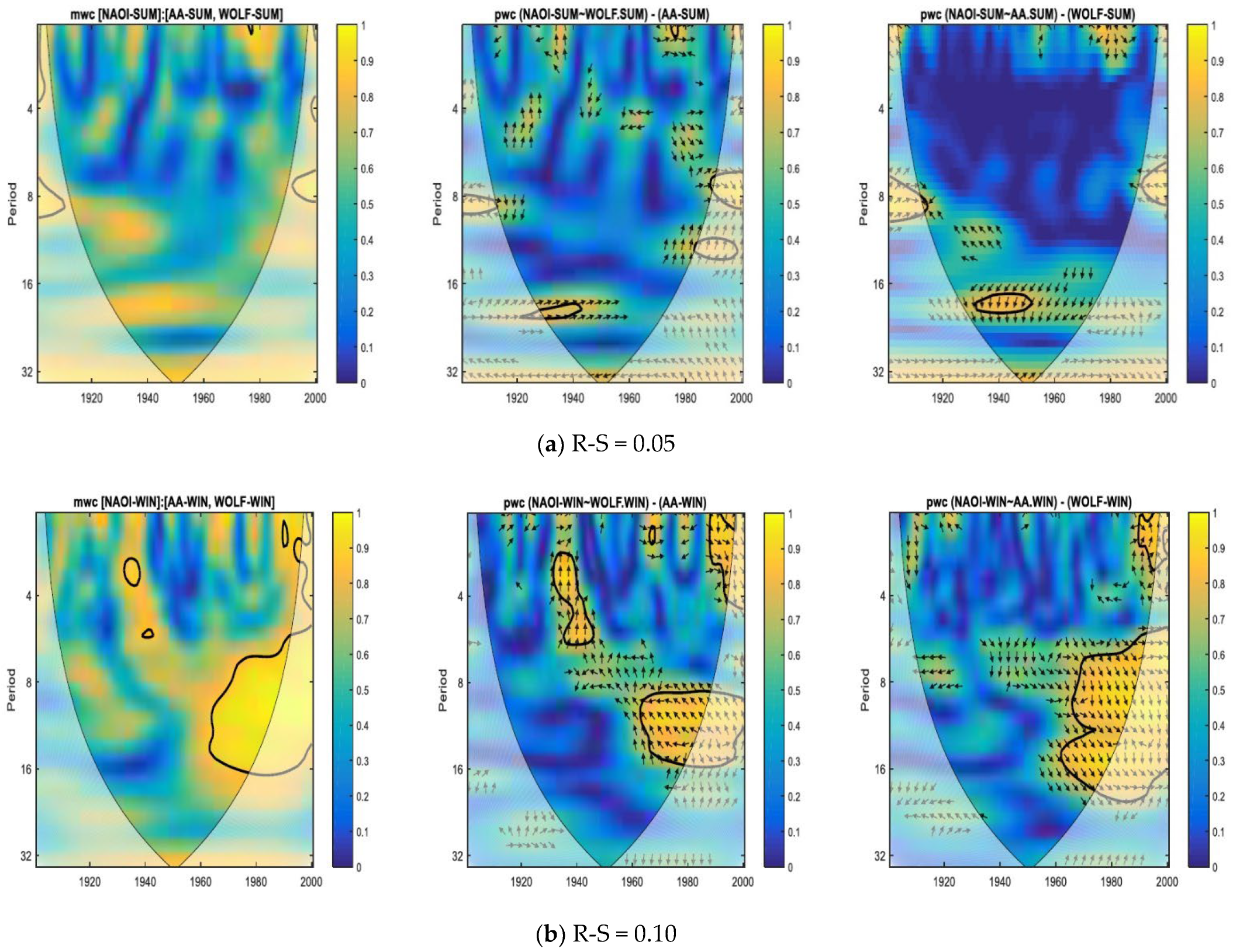
Figure 4a,b show the results obtained by wavelet analysis for NAOI in summer with low R-S (0.05) and a relatively high R-S (0.10) situation found in winter, with both cases at lag = 0. If for summer, the wavelet analysis highlights only isolated cases with significant coherence, in the case of winter (Figure 4b), both the mwc and pwc highlight a significant coherence, and between NAOI in winter and solar/geomagnetic indices, for periods around the 11-year solar cycle (Schwabe) after the 1970s. This significant coherence after the 1970s could either be because of changes of NAO (Beniston and Jungo) [42], or because of certain changes that had taken place in the so-called “top-down” and “bottom-up” of the solar influence mechanisms, as shown in (Gray et al.; Lin et al.; Kuroda et al.) [107,108,109].
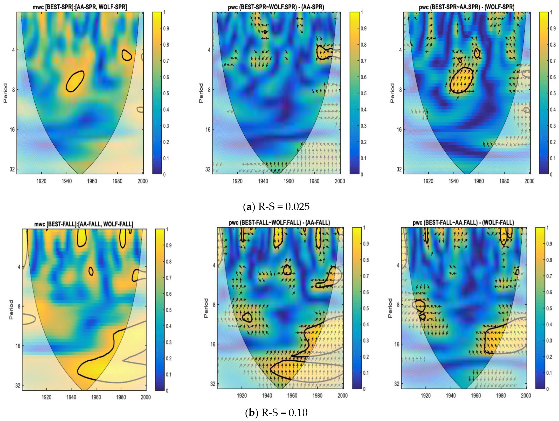
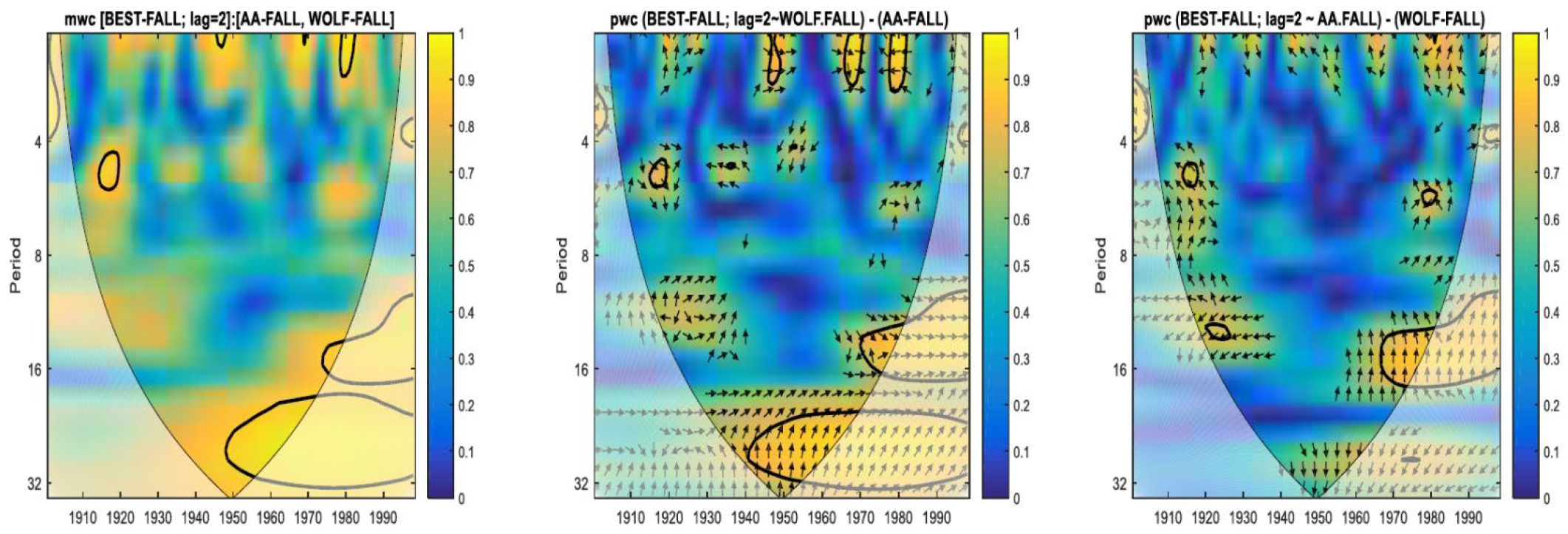
In Figure 5, where the results of the wavelet analysis for the BEST climate index are presented, it can be seen that for the first case, R-S low (0.025) in the spring season (Figure 5a), both mwc and pwc do not show significant coherence except for very isolated cases. On the other hand, for the autumn season (Figure 5b), it is observed that the two predictors considered together produce a greater coherence than if only one is considered and the other is excluded. This is especially true for the coherence corresponding to the double solar cycle (Hale’s cycle) and especially after the 1940s.
Investigations regarding the response of the BEST climate index to solar activity do not really exist to our knowledge, probably because this index is highly correlated with ENSO [52]. As shown in the publication [52], Smith and Sardeshmukh [53] joined the SOI and Nino 3.4 SST (Sea Surface Temperature) anomalies into a “Bivariate ENSO Timeseries” (BEST) index in the simplest possible fashion.
Fang et al. [44] explored the teleconnections between spring drought, winter drought, and climate indices on the one hand and the sunspot number on the other, by using (XWT) and (WTC) analyses. BEST is among the climate indices used. The results are discussed according to the coherence wavelet between precipitation and BEST, or between precipitation and sunspot number.
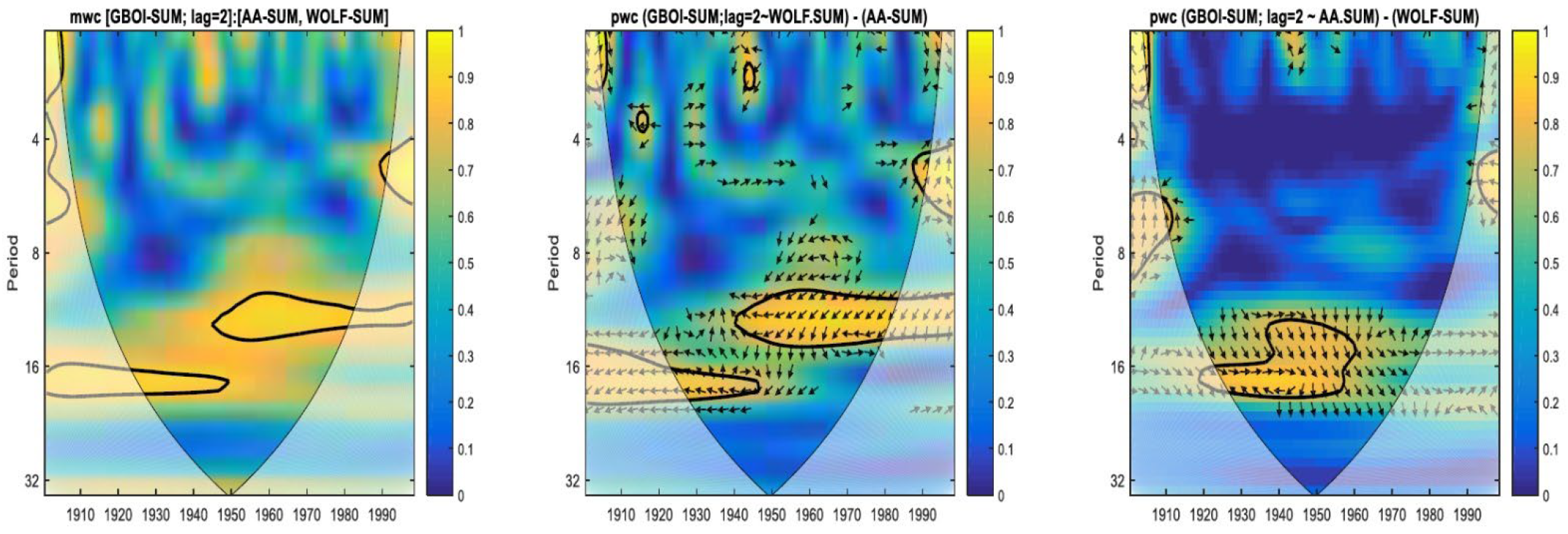
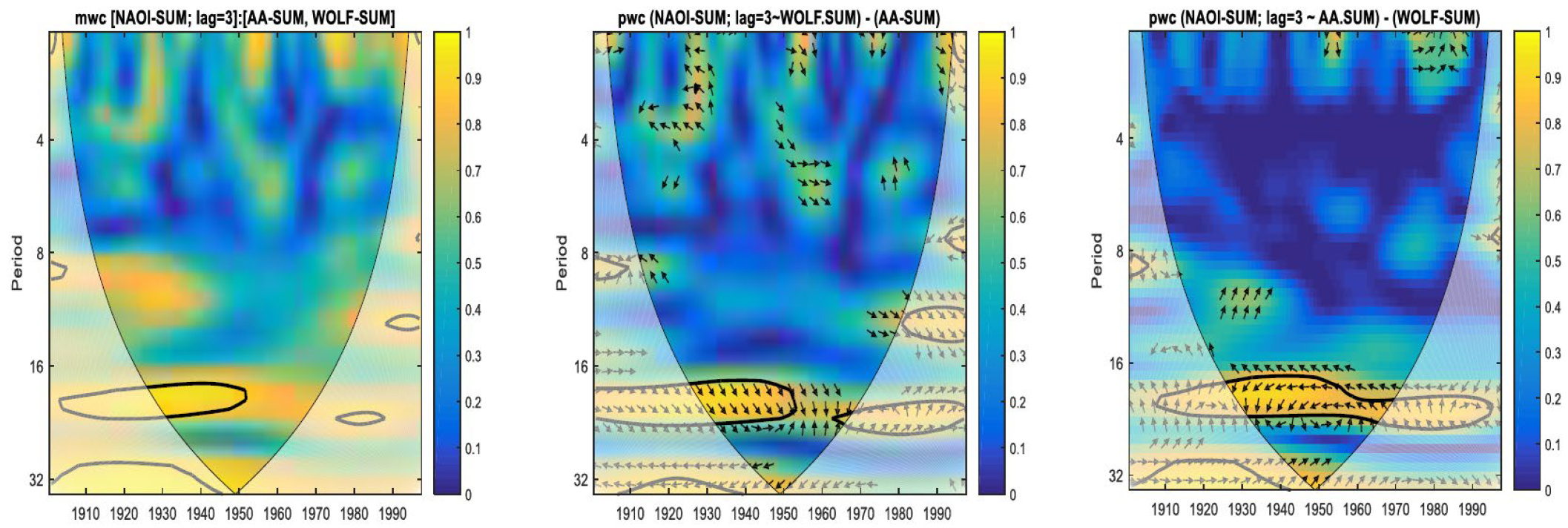
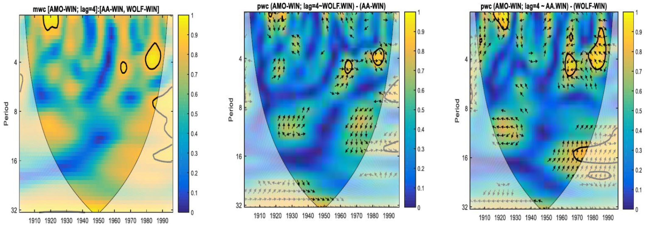
In the following section, we will discuss the results obtained by wavelet coherence (Figure 6, Figure 7, Figure 8, Figure 9 and Figure 10) for five more representative cases, with different lags between predictors and predictand. These situations were selected taking into account both the R-S (to be high) and the highest values of TC presented in Figure 2. Thus the climatic indices were selected: GBOI summer at lag 2 (Figure 6), NAOI, summer at a lag of 2 and 3 years (Figure 7 and Figure 8), BEST in autumn at lag = 2 (Figure 9) and AMO in winter at lag = 4 years (Figure 10). Regarding the results from the Figure 6, where the time-frequency distribution at lag 2 for GBOI summer is presented, it is noted that this distribution does not differ much from the distribution at lag = 0 (Figure 3b), as is evidenced by R-S and TC as well. If we also take into account the values of NLR from Figure 1 at lag = 2, the analysis by mwc and pwc highlights the greater contribution of the Wolf number compared to that of the geomagnetic index aa.
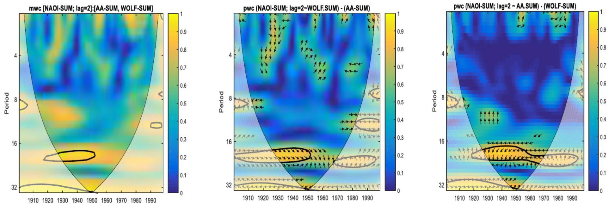
If we compare the coherences between summer NAOI with the two predictors at lags 2 and 3 (Figure 7 and Figure 8), it can be seen that both the aa and Wolf number contribute to the coherence obtained by mwc for periodicities around the double solar cycle, especially for the years 1930–1950.
For the wavelet coherence distribution for BEST during autumn (Figure 9), it is obvious that the consideration of the two predictors together with a lag of 2 years leads to the extension of the significance coherence areas. This is also confirmed by R-S, which in this case, has a relatively high value of 0.18 compared to the other cases.
Related to the response of the AMO climate index in winter at a delay of 4 years compared to the solar/geomagnetic activity (Figure 10), as in the case of BEST, the coherence through mwc is more significant, compared to that obtained through pwc by excluding one among the predictors. Therefore, it is necessary to consider both predictors for estimating the behavior of AMO, especially since they can be used in an equation, as with regression, for example, because the R-S for this season at lag 4 has a value of approximately 0.2 (Figure 2).
However, when two or more predictors are considered together and we want to filter them for a certain frequency band, the difference between synergy and redundancy must be checked again. As demonstrated in Mares et al. [66], in the case of the GBOI climate index, when a bandpass filter was applied, the R-S became negative, so the predictors by filtering become redundant.
Although the results obtained in this study do not all have a high level of statistical significance, we will consider the cases in which the statistical significance is high enough in our future studies. For the estimation of areas of interest on a local or regional scale, such as the Danube basin, the indicators of solar/geomagnetic activity must be considered together with large-scale climate indices, as predictors for the predictand such as the discharge of the Danube. Examples in this sense are found in the investigations [44,47,51].

4. Conclusions

In the present study, the influence of solar/geomagnetic activity, quantified by the Wolf number and by the aa geomagnetic index, respectively, on the climate indices (CIs), was investigated by applying up-to-date methods that highlight non-linear and non-stationary links.
First, the non-linear correlation coefficients, based on mutual information, have clearly pointed out, with few exceptions, that the indicators designed to describe solar/geomagnetic activity, simultaneously or with certain lags, influence the climatic indices in a non-linear way. It was found that most cases with significant signals (CL~95%) of non-linear nature of the solar activity are manifested during the autumn season on GBOI, AO, AMO and TNI, at lags of 3, 5, 4 and 5 years, respectively. For the same autumn season, the influence of the geomagnetic activity is significant with a CL > 95% only on AMO at a lag of 4 years. However, AMO during the winter season is influenced by the geomagnetic activity at lags 0, 1 and 4 years with associated CL > 95%.
In order to see if the two indices that characterize solar/geomagnetic activit, can be used together as predictors for a climate index (predictand), the difference between synergy and redundancy (S-R) was estimated, in which the total correlation (TC) between the three variables was also associated. For certain cases, either with small or larger S-R, details of the coherence between the three variables were obtained by mwc, or considering only one predictor, excluding the influence of the other by applying pwc. Thus, details on the frequency-time distribution were obtained.
By comparing the coherence obtained by mwc with that obtained by pwc, it can be concluded whether the information brought by the two predictors together is more important for the predictand, or the information of only one of the predictors is better than the two taken together. The results obtained in the present study differ depending on the season, the predictand and the lag used.
In general, the highest values of R-S were found at different lags, compared to lag 0 (that is, in the case of simultaneous consideration of the predictor and the predictand). For example, the highest R-S value was obtained during autumn for the AMO climate index considered at the 4-year lag, compared to the solar/geomagnetic activity. The coherence through mwc and pwc clearly indicates that the two predictors have a greater coherence with the predictand when they are considered together, than when they are taken separately. However, when two or more predictors are considered together and we want to filter them for a certain frequency band, the difference between synergy and redundancy must be checked again, as the predictors by filtering become redundant.

Author Contributions

Conceptualization, C.M.; investigation, C.M., V.D. and I.M.; methodology, C.M., I.M. and V.D.; writing—original draft preparation, C.M., V.D., I.M. and C.D.; supervision and validation C.D. All authors have read and agreed to the published version of the manuscript.

Funding

This research received no external funding.

Institutional Review Board Statement

Not applicable.

Informed Consent Statement

Not applicable.

Data Availability Statement

Not applicable.

Acknowledgments

The codes for calculating pwc can be downloaded from https://figshare.com/s/bc97956f43fe5734c784 (accessed on 1 October 2022), Hu and Si (2021). The author thanks the anonymous reviewers for relevant suggestions to improve this study.

Conflicts of Interest

The authors declare no conflict of interest.

Abbreviations

The following abbreviations are used in this manuscript:
aa(AA)Geomagnetic index
AMOAtlantic Multidecadal Oscillation
AOArctic Oscillation
BESTBivariate ENSO Timeseries
CisClimate Indices
CLConfidence levels
ENSOEl Niño–Southern Oscillation
GBOIGreenland-Balkan Oscillation Index
IPCCAR6Intergovernmental Panel on Climate Change’s Sixth Assessment Report
MEIMultivariates ENSO Index
MwcMultiple wavelet coherence
NAOINorth Atlantic Oscillation Index
NLRNon-linear correlation coefficient
PwcPartial wavelet coherence
QBOQuasi-Biennial Oscillation
RPearson correlation coefficient
SOISouthern Oscillation Index
SLPSea Level Pressure
S-RSynergy and minus Redundancy
SSTSea Surface Temperature
TCTotal Correlation
TNITrans-Niño Index
WTCWavelet Coherence
WOLFWolf Number
XWTCross Wavelet Spectrum

References

  1. Haigh, J.D.; Blackburn, M.; Day, R. The response of tropospheric circulation to perturbations in lower-stratospheric temperature. J. Clim. 2005, 18, 3672–3685. [Google Scholar] [CrossRef]
  2. Haigh, J.D. Mechanisms for solar influence on the Earth’s climate. In Climate and Weather of the Sun-Earth System (CAWSES): Selected Papers from the 2007 Kyoto Symposium; Tsuda, T., Fujii, R., Shibata, K., Geller, M.A., Eds.; TERRAPUB: Tokyo, Japan, 2009; pp. 231–256. [Google Scholar]
  3. Herschel, W. Observations tending to investigate the nature of the Sun, in order to find the causes or symptoms of its variable emission of light and heat: With remarks on the use that may possibly be drawn from solar observations. Philos. Trans. R. Soc. Lond. 1801, 91, 265–318. [Google Scholar] [CrossRef] [Green Version]
  4. Mitchell, J.M. An Overview of Climatic Variability and its Causal Mechanisms. Quat. Res. 1976, 6, 481–493. [Google Scholar] [CrossRef]
  5. Prestes, A.; Rigozo, N.R.; Echer, E.; Vieira, L.E.A. Spectral analysis of sunspot number and geomagnetic indices (1868–2001). J. Atmos. Sol.-Terr. Phys. 2006, 68, 182–190. [Google Scholar] [CrossRef]
  6. Woollings, T.; Lockwood, M.; Masato, G.; Bell, C.; Gray, L. Enhanced signature of solar variability in Eurasianwinter climate. Geophys. Res. Lett. 2010, 37, L20805. [Google Scholar] [CrossRef]
  7. Scafetta, N.; Bianchini, A. The planetary theory of solar activity variability: A review. Front. Astron. Space Sci. 2022, 9, 937930. [Google Scholar] [CrossRef]
  8. Hassan, D.; Iqbal, A.; Hassan, S.A.; Abbas, S.; Ansari, M.R.K. Sunspots and ENSO relationship using Markov method. J. Atmos. Sol.-Terr. Phys. 2016, 137, 53–57. [Google Scholar] [CrossRef]
  9. von der Heydt, A.; Ashwin, S.P.; Camp, C.D.; Crucifix, M.; Dijkstra, H.A.; Ditlevsen, P.; Lenton, T.M. Quantification and interpretation of the climate variability record. Glob. Planet. Chang. 2021, 197, 103399. [Google Scholar] [CrossRef]
  10. Song, Y.; Li, Z.; Zhou, Y.; Bi, X.; Sun, B.; Xiao, T.; Suo, L.; Zhang, W.; Xiao, Z.; Wang, C. The Influence of Solar Activity on Snow Cover over the Qinghai–Tibet Plateau and ItsMechanism Analysis. Atmosphere 2022, 13, 1499. [Google Scholar] [CrossRef]
  11. Gil-Alana, L.A.; Yaya, O.S.; Shittu, O.I. Global temperatures and sunspot numbers. Are they related? Phys. A Stat. Mech. Its Appl. 2014, 413, 329–342. [Google Scholar] [CrossRef]
  12. Ajayi, O.G.; Ibik, A.L.; Odumosu, J.O.; Babalola, K.H.; Adesina, E.A. Investigation of the Impact of Sunspots on Earth’s Climate Sustainable Built Environment and Climate change. In The Challenges of Post 2015 Development Agenda; School of Environmental Technology International Conference (SETIC); Federal University of Technology (FUT): Minna, Nigeria, 2016; Available online: https://www.researchgate.net/publication/343878002 (accessed on 5 July 2022).
  13. Chiodo, G.; Oehrlein, J.; Polvani, L.M.; Fyfe, J.C.; Smith, A.K. Insignificant influence of the 11-year solar cycle on the North Atlantic Oscillation. Nat. Geosci. 2019, 12, 94–99. [Google Scholar] [CrossRef]
  14. Courtillot, V.; Gallet, Y.; Le Mouël, J.L.; Fluteau, F.; Genevey, A. Are there connections between the Earth’s magnetic field and climate? Earth Planet. Sc. Lett. 2007, 253, 328–339. [Google Scholar] [CrossRef]
  15. Gray, L.J.; Beer, J.; Geller, M.; Haigh, J.D.; Lockwood, M.; Matthes, K.; Cubasch, U.; Fleitmann, D.; Harrison, G.; Hood, L.; et al. Solar influences on climate. Rev. Geophys. 2010, 48, RG4001. [Google Scholar] [CrossRef] [Green Version]
  16. Gray, L.J.; Scaife, A.A.; Mitchell, D.M.; Osprey, S.; Ineson, S.; Hardiman, S.; Butchart, N.; Knight, J.; Sutton, R.; Kodera, K. A lagged response to the 11 year solar cycle in observed winter Atlantic/European weather patterns. J. Geophys. Res. Atmos. 2013, 118, 13405–13420. [Google Scholar] [CrossRef] [Green Version]
  17. Lorenz, E.N. Energy and Numerical Weather Prediction. Tellus 1960, 12, 364–373. [Google Scholar] [CrossRef] [Green Version]
  18. Holton, J.R. An Introduction to Dynamic Meteorology; Academic Press: New York, NY, USA, 1972. [Google Scholar]
  19. Willis, D.M. The Energetics of Sun-Weather Relationships-Magnetospheric Processes. J. Atmos. Terr. Phys. 1976, 38, 685–698. [Google Scholar] [CrossRef]
  20. Larsen, M.F.; Kelley, M.C. Available Potential Energy in the Middle Atmosphere as it Relates to the Sun-Weather Effect. In Solar-Terrestrial Influences on Weather and Climate; McCormac, B.M., Seliga, T.A., Eds.; Springer: Dordrecht, The Netherlands, 1979; pp. 145–147. [Google Scholar] [CrossRef]
  21. Peixoto, J.P.; Oort, A.H. Physics of Climate; American Institute of Physics: College Park, MD, USA, 1992; p. 520. [Google Scholar]
  22. Labitzke, K.; van Loon, H. Associations between the 11‐year solar cycle, the QBO and the atmosphere. Part I: The troposphere and stratosphere in the northern hemisphere in winter. J. Atmos. Terr. Phys. 1988, 50, 197–206. [Google Scholar] [CrossRef]
  23. Foukal, P. A comparison of variable solar total and ultraviolet irradiance outputs in the 20th century. Geophys. Res. Lett. 2002, 29, 4-1–4-4. [Google Scholar] [CrossRef]
  24. Kodera, K.; Coughlin, K.; Arakawa, O. Possible modulation of the connection between the Pacific and Indian Ocean variability by the solar cycle. Geophys. Res. Lett. 2007, 34, L03710. [Google Scholar] [CrossRef]
  25. Meehl, G.A.; Arblaster, J.M.; Matthes, K.; Sassi, F.; van Loon, H. Amplifying the Pacific Climate System Response to a Small 11-Year Solar Cycle Forcing. Science 2009, 325, 1114–1118. [Google Scholar] [CrossRef] [Green Version]
  26. Benestad, R.E. Low solar activity is blamed for winter chill over Europe. Environ. Res. Lett. 2010, 5, 021001. [Google Scholar] [CrossRef]
  27. Friis-Christensen, E.; Lassen, K. Length of the solar cycle: An indicator of solar activity closely associated with climate. Science 1991, 254, 698–700. [Google Scholar] [CrossRef] [PubMed] [Green Version]
  28. Lean, J.; Beer, J.; Bradley, R.S. Reconstruction of solar irradiance since 1610: Implications for climate change. Geophys. Res. Lett. 1995, 22, 3195–3198. [Google Scholar] [CrossRef] [Green Version]
  29. Haigh, J.D. The effects of solar variability on the Earth’s climate. Philos. Trans. R. Soc. Lond. Ser. A Math. Phys. Eng. Sci. 2003, 361, 95–111. [Google Scholar] [CrossRef]
  30. Lockwood, M. Solar Influence on Global and Regional Climates. Surv. Geophys. 2012, 33, 503–534. [Google Scholar] [CrossRef] [Green Version]
  31. Saltzman, B. A Survey of Sttisticl-Dynamical Models of the Terrestrial Climate. In Advance in Geophysics; Saltzman, B., Ed.; Academic Press: New York, NY, USA; San Francisco, CA, USA; London, UK, 1978; pp. 278–282. [Google Scholar]
  32. Hunt, B.G. Nonlinear Influences-A Key to Short-Term Climatic Perturbations. J. Atmos. Sci. 1988, 45, 387–395. [Google Scholar] [CrossRef]
  33. Chapanov, Y. ENSO Variations Driven by Solar Cycles, Expressed by N-S Solar Asymmetry.Topic: Solar Influences on the Lower Atmosphere and Climate. In Proceedings of the Eleventh Workshop Solar Influences on the Magnetosphere, Ionosphere and Atmosphere, Primorsko, Bulgaria, 3–7 June 2019; p. 152. Available online: http://ws-sozopol.stil.bas.bg (accessed on 5 May 2022).
  34. Yndestad, H.; Solheim, J.E. The influence of solar system oscillation on the variability of the total solar irradiance. New Astron. 2017, 51, 135–152. [Google Scholar] [CrossRef] [Green Version]
  35. Clette, F.; Svalgaard, L.; Vaquero, J.M.; Cliver, E.W. Revisiting the Sunspot Number. Space Sci. Rev. 2014, 186, 35–103. [Google Scholar] [CrossRef] [Green Version]
  36. Masson-Delmotte, V.; Zhai, P.; Pirani, A.; Connors, S.L.; Péan, C.; Berger, S.; Caud, N.; Chen, Y.; Goldfarb, L.; Gomis, M.I.; et al. IPCC, Climate Change 2021: The Physical Science Basis. Contribution of Working Group I to the Sixth Assessment Report of the Intergovernmental Panel on Climate Change; University Press: Cambridge, UK; New York, NY, USA, 2021; p. 2391. [Google Scholar] [CrossRef]
  37. Chapman, S.C.; McIntosh, S.W.; Leamon, R.J.; Watkins, N.W. Quantifying the solar cycle modulation of extreme space weather. Geophys. Res. Lett. 2020, 47, e2020GL087795. [Google Scholar] [CrossRef]
  38. Katsavrias, C.; Papadimitriou, C.; Hillaris, A.; Balasis, G. Application of Wavelet Methods in the Investigation of Geospace Disturbances: A Review and an Evaluation of the Approach for Quantifying Wavelet Power. Atmosphere 2022, 13, 499. [Google Scholar] [CrossRef]
  39. Mawad, R.; Fathy, M.; Ghamry, E. The Simultaneous Influence of the Solar Wind and Earth’s Magnetic Field on the Weather. Universe 2022, 8, 424. [Google Scholar] [CrossRef]
  40. Addison, P. The little wave with the big future. Phys. World 2004, 17, 35. [Google Scholar] [CrossRef]
  41. Stenseth, N.C.; Ottersen, G.; Hurrell, J.W.; Mysterud, A.; Lima, M.; Chan, K.-S.; Yoccoz, N.G.; Adlandsvik, B. Studying climate effects on ecology through the use of climate indices: The North Atlantic Oscillation, El Nino Southern Oscillation and beyond. Proc. R. Soc. Lon. Ser. B Biol. Sci. 2003, 270, 2087–2096. [Google Scholar] [CrossRef] [PubMed] [Green Version]
  42. Beniston, M.; Jungo, P. Shifts in the distributions of pressure, temperature and moisture and changes in the typical weather patterns in the Alpine region in response to the behavior of the North Atlantic Oscillation. Theor. Appl. Climatol. 2002, 71, 29–42. [Google Scholar] [CrossRef] [Green Version]
  43. Zanchettin, D.; Rubino, A.; Traverso, P.; Tomasino, M. Impact of variations in solar activity on hydrological decadal patterns in northern Italy. J. Geophys. Res. Atmos. 2008, 113, D12. [Google Scholar] [CrossRef] [Green Version]
  44. Fang, G.; Li, X.; Xu, M.; Wen, X.; Huang, X. Spatiotemporal Variability of Drought and Its Multi-Scale Linkages with Climate Indices in the Huaihe River Basin, Central China and East China. Atmosphere 2021, 12, 1446. [Google Scholar] [CrossRef]
  45. López-Moreno, J.I.; Vicente-Serrano, S.M.; Morán-Tejeda, E.; Lorenzo-Lacruz, J.; Kenawy, A.; Beniston, M. Effects of the North Atlantic Oscillation (NAO) on combined temperature and precipitation winter modes in the Mediterranean mountains: Observed relationships and projections for the 21st century. Glob. Planet. Chang. 2011, 77, 62–76. [Google Scholar] [CrossRef]
  46. Vyshkvarkova, E.; Sukhonos, O. Compound Extremes of Air Temperature and Precipitation in Eastern Europe. Climate 2022, 10, 133. [Google Scholar] [CrossRef]
  47. Dobrica, V.; Demetrescu, C.; Mares, I.; Mares, C. Long-term evolution of the Lower 608 Danube discharge and corresponding climate variations: Solar signature imprint. Theor. Appl. Climatol. 2018, 133, 985–996. [Google Scholar] [CrossRef]
  48. Le Mouël, J.L.; Lopes, F.; Courtillot, V. A solar signature in many climate indices. J. Geophys. Res. Atmos. 2019, 124, 2600–2619. [Google Scholar] [CrossRef]
  49. Drews, A.; Huo, W.; Matthes, K.; Kodera, K.; Kruschke, T. The Sun’s role in decadal climate predictability in the North Atlantic. Atmos. Chem. Phys. 2022, 22, 7893–7904. [Google Scholar] [CrossRef]
  50. Nuzhdina, M.A. Connection between ENSO phenomena and solar and geomagnetic activity. Nat. Hazards Earth Syst. Sci. 2002, 2, 83–89. [Google Scholar] [CrossRef] [Green Version]
  51. Fu, C.; James, A.L.; Wachowiak, M.P. Analyzing the combined influence of solar activity and El Niño on streamflow across southern Canada. Water Resour. Res. 2012, 48, W05507. [Google Scholar] [CrossRef]
  52. Wolter, K.; Timlin, M.S. El Niño/Southern Oscillation behaviour since 1871 as diagnosed in an extended multivariate ENSO index (MEI.ext). Int. J. Climatol. 2011, 31, 1074–1087. [Google Scholar] [CrossRef]
  53. Smith, C.A.; Sardeshmukh, P.D. The Effect of ENSO on the Intraseasonal Variance of Surface Temperature in Winter. Int. J. Climatol. A J. R. Meteorol. Soc. 2000, 20, 1543–1557. [Google Scholar] [CrossRef]
  54. Campuzano, S.A.; De Santis, A.; Pavo´n-Carrasco, F.J.; Osete, M.L.; Qamili, E. New perspectives in the study of the Earth’s magnetic field and climate connection: The use of transfer entropy. PLoS ONE. 2018, 13, e0207270. [Google Scholar] [CrossRef] [Green Version]
  55. Vu, T.M.; Mishra, A.K.; Konapala, G. Information Entropy Suggests Stronger Nonlinear Associations between Hydro-Meteorological Variables and ENSO. Entropy 2018, 20, 38. [Google Scholar] [CrossRef] [Green Version]
  56. Paluš, M.; Novotná, D. Common oscillatory modes in geomagnetic activity, NAO index and surface air temperature records. J. Atmos. Sol.-Terr. Phys. 2007, 69, 2405–2415. [Google Scholar] [CrossRef]
  57. Wing, S.; Johnson, J.; Vourlidas, A. Information theoretic approach to discovering causalities in the solar cycle. Astrophys. J. 2018, 854, 85. [Google Scholar] [CrossRef]
  58. Wing, S.; Johnson, J.R. Applications of information theory in solar and space physics. Entropy 2019, 21, 140. [Google Scholar] [CrossRef] [Green Version]
  59. Goodwell, A.E.; Jiang, P.; Ruddell, B.L.; Kumar, P. Debates—Does information theory provide a new paradigm for Earth science? Causality, interaction, and feedback. Water Resour. Res. 2020, 56, e2019WR024940. [Google Scholar] [CrossRef] [Green Version]
  60. Lorenzo-Lacruz, J.; Morán-Tejeda, E.; Vicente-Serrano, S.M.; Hannaford, J.; García, C.; Peña-Angulo, D.; Murphy, C. Streamflow frequency changes across western Europe and interactions with North Atlantic atmospheric circulation patterns. Glob. Planet. Chang. 2022, 212, 103797. [Google Scholar] [CrossRef]
  61. Sonechkin, D.M.; Vakulenko, N.V. Polyphony of Short-Term Climatic Variations. Atmosphere 2021, 12, 1145. [Google Scholar] [CrossRef]
  62. Rathinasamy, M.; Agarwal, A.; Parmar, V.; Khosa, R.; Bairwa, A. Partial wavelet coherence analysis for understanding the standalone relationship between Indian Precipitation and Teleconnection patterns. arXiv 2017, arXiv:1702.06568. [Google Scholar]
  63. Labat, D. Recent advances in wavelet analyses: Part 1. A review of concepts. J. Hydrol. 2005, 314, 275–288. [Google Scholar] [CrossRef]
  64. Moore, J.; Grinsted, A.; Jevrejeva, S. Is there evidence for sunspot forcing of climate at multi-year and decadal periods? Geophys. Res. Lett. 2006, 33, L17705. [Google Scholar] [CrossRef] [Green Version]
  65. Mares, C.; Mares, I.; Dobrica, V.; Demetrescu, C. Quantification of the direct solar impact on some components of the hydroclimatic system. Entropy 2021, 23, 691. [Google Scholar] [CrossRef] [PubMed]
  66. Mares, I.; Dobrica, V.; Mares, C.; Demetrescu, C. Assessing the solar variability signature in climate variables by information theory and wavelet coherence. Sci. Rep. 2021, 11, 11337. [Google Scholar] [CrossRef]
  67. Mares, I.; Mares, C.; Dobrica, V.; Demetrescu, C. Selection of Optimal Palmer Predictors for Increasing the Predictability of the Danube Discharge: New Findings Based on Information Theory and Partial Wavelet Coherence Analysis. Entropy 2022, 24, 1375. [Google Scholar] [CrossRef]
  68. Mallat, S.A. Wavelet Tour of Signal Processing; Academic-Press: Cambridge, MA, USA, 1998. [Google Scholar]
  69. Tary, J.B.; Herrera, R.H.; Han, J.; van der Baan, M. Spectral estimation—What is new? What is next? Rev. Geophys. 2014, 52, 723–749. [Google Scholar] [CrossRef]
  70. Ghil, M.; Allen, M.R.; Dettinger, M.D.; Ide, K.; Kondrashov, D.; Mann, M.E.; Robertson, A.W.; Saunders, A.; Tian, Y.; Varadi, F.; et al. Advanced spectral methods for climatic time series. Rev. Geophys. 2002, 40, 3-1–3-41. [Google Scholar] [CrossRef] [Green Version]
  71. Si, B.C. Spatial scaling analyses of soil physical properties: A review of spectral and wavelet methods. Vadose Zone J. 2008, 7, 547–562. [Google Scholar] [CrossRef] [Green Version]
  72. Sleziak, P.; Hlavčová, K.; Szolgay, J. Advantages of a time series analysis using wavelet transform as compared with a Fourier analysis. Slovak J. Civ. Eng. 2015, 23, 30. [Google Scholar] [CrossRef] [Green Version]
  73. Hood, L.; Schimanke, S.; Spangehl, T.; Bal, S.; Cubasch, U. The surface climate response to 11-yr solar forcing during northern winter: Observational analyses and comparisons with GCM simulations. J. Clim. 2013, 26, 7489–7506. [Google Scholar] [CrossRef] [Green Version]
  74. Mares, I.; Mares, C.; Mihailescu, M. Stochastic modeling of the connection between sea level pressure and discharge in the Danube lower basin by means of Hidden Markov Model. EGU Gen. Assem. Conf. Abstr. 2013, 15, EGU2013-7606. [Google Scholar]
  75. Hurrell, J.W. Decadal trends in the North Atlantic Oscillation and relationships to regional temperature and precipitation. Science 1995, 269, 676–679. [Google Scholar] [CrossRef] [Green Version]
  76. Thompson, D.W.J.; Wallace, J.M. The Arctic Oscillation signature in the wintertime geopotential height and temperature fields. Geophys. Res. Lett. 1998, 25, 1297–1300. [Google Scholar] [CrossRef] [Green Version]
  77. Enfield, D.B.; Mestas-Nunez, A.M.; Trimble, P.J. The Atlantic Multidecadal Oscillation and its relationship to rainfall and river flows in the continental U.S. Geophys. Res. Lett. 2001, 28, 2077–2080. [Google Scholar] [CrossRef] [Green Version]
  78. Ropelewski, C.F.; Jones, P.D. An extension of the Tahiti-Darwin Southern Oscillation Index. Mon. Weather Rev. 1987, 115, 2161–2165. [Google Scholar] [CrossRef]
  79. Trenberth, K.E.; Stepaniak, D.P. Indices of El Niño Evolution. J. Clim. 2001, 14, 1697–1701. Available online: https://www.jstor.org/stable/26247387 (accessed on 27 October 2022). [CrossRef]
  80. Mares, C.; Mares, I.; Mihailescu, M. Identification of extreme events using drought indices and their impact on the Danube lower basin discharge. Hydrol. Proc. 2016, 30, 3839–3854. [Google Scholar] [CrossRef]
  81. Mares, I.; Dobrica, V.; Demetrescu, C.; Mares, C. Hydrological response in the Danube lower basin to some internal and external climate forcing factors. Hydrol. Earth Syst. Sci. Discuss. 2016. preprint. [Google Scholar] [CrossRef] [Green Version]
  82. Mares, I.; Mares, C.; Dobrica, V.; Demetrescu, C. Comparative study of statistical methods to identify a predictor for discharge at Orsova in the Lower Danube Basin. Hydrol. Sci. J. 2020, 65, 371–386. [Google Scholar] [CrossRef]
  83. Lüdecke, H.; Müller-Plath, G.; Wallace, M.G.; Lüning, S. Decadal and multidecadal natural variability of African rainfall. J. Hydrol. Reg. Stud. 2021, 34, 100795. [Google Scholar] [CrossRef]
  84. Laurenz, L.; Lüdecke, H.-J.; Lüning, S. Influence of solar activity changes on European rainfall. J. Atmos. Sol.-Terr. Phys. 2019, 185, 29–42. [Google Scholar] [CrossRef]
  85. Khan, S.; Ganguly, A.R.; Bandyopadhyay, S.; Saigal, S.; Erickson, D.J.; Protopopescu, V.; Ostrouchov, G. Nonlinear statistics reveals stronger ties between ENSO and the tropical hydrological cycle. Geophys. Res. Lett. 2006, 33, L24402. [Google Scholar] [CrossRef] [Green Version]
  86. Steuer, R.; Kurths, J.; Daub, C.O.; Weise, J.; Selbig, J. The mutual information: Detecting and evaluating dependencies between variables. Bioinformatics 2002, 18, S231–S240. [Google Scholar] [CrossRef] [Green Version]
  87. Theiler, J.; Eubank, S.; Longtin, A.; Galdrikian, B.; Farmer, J.D. Testing for nonlinearity in time series: The method of surrogate data. Phys. D Nonlinear Phenom. 1992, 58, 77–94. [Google Scholar] [CrossRef] [Green Version]
  88. Timme, N.; Alford, W.; Flecker, B.; Beggs, J.M. Synergy, redundancy, and multivariate information measures: An experimentalist’s perspective. J. Comput. Neurosci. 2014, 36, 119–140. [Google Scholar] [CrossRef]
  89. Mihanovic, H.; Orlie, M.; Pasaria, Z. Diurnal thermocline oscillations driven by tidal flow around an island in the Middle Adriatic. J. Mar. Syst. 2009, 78, S157–S168. [Google Scholar] [CrossRef]
  90. Torrence, C.; Compo, G.P. A practical guide to wavelet analysis. Bull. Am. Meteorol. Soc. 1998, 79, 61–78. [Google Scholar] [CrossRef]
  91. Sreedevi, V.; Adarsh, S.; Nourani, V. Multiscale coherence analysis of reference evapotranspiration of north-western Iran using wavelet transform. J. Water Clim. Chang. 2022, 13, 505–521. [Google Scholar] [CrossRef]
  92. Gu, X.; Sun, H.; Zhang, Y.; Zhang, S.; Lu, C. Partial Wavelet Coherence to Evaluate Scale-dependent Relationships Between Precipitation/Surface Water and Groundwater Levels in a Groundwater System. Water Resour. Manag. 2022, 36, 2509–2522. [Google Scholar] [CrossRef]
  93. Hu, W.; Si, B.C. Technical Note: Improved partial wavelet coherency for understanding scale- specific and localized bivariate relationships in geosciences. Hydrol. Earth Syst. Sci. 2021, 25, 321–331. [Google Scholar] [CrossRef]
  94. Zhou, Z.; Liu, S.; Ding, Y.; Fu, Q.; Wang, Y.; Cai, H.; Shi, H. Assessing the responses of vegetation to meteorological drought and its influencing factors with partial wavelet coherence analysis. J. Environ. Manag. 2022, 311, 114879. [Google Scholar] [CrossRef] [PubMed]
  95. Firouzi, S.; Wang, X. The interrelationship between order flow, exchange rate, and the role of American economic news. N. Am. J. Econ. Financ. 2021, 58, 101492. [Google Scholar] [CrossRef]
  96. Hu, W.; Si, B.C. Multiple wavelet coherence for untangling scale-specific and localized multivariate relationships in geosciences. Hydrol. Earth Syst. Sci. 2016, 20, 3183–3191. [Google Scholar] [CrossRef] [Green Version]
  97. Grinsted, A.; Moore, J.C.; Jevrejeva, S. Application of the cross wavelet transform and wavelet coherence to geophysical time series. Nonlinear Process. Geophys. 2004, 11, 561–566. [Google Scholar] [CrossRef]
  98. Maraun, D.; Kurths, J.; Holschneider, M. Nonstationary Gaussian processes in wavelet domain: Synthesis, estimation, and significance testing. Phys. Rev. E 2007, 75, 016707. [Google Scholar] [CrossRef] [Green Version]
  99. Jevrejeva, S.; Moore, J.C.; Grinsted, A. Influence of the Arctic Oscillation and ElNiño-Southern Oscillation (ENSO) on ice conditions in the Baltic Sea: The wavelet approach. J. Geophys. Res. 2003, 108, 4677. [Google Scholar] [CrossRef]
  100. Torrence, C.; Webster, P. Interdecadal changes in the ESNO-Monsoon System. J. Clim. 1999, 12, 2679–2690. [Google Scholar] [CrossRef]
  101. Zaidan, M.A.; Haapasilta, V.; Relan, R.; Paasonen, P.; Kerminen, V.-M.; Junninen, H.; Kulmala, M.; Foster, A.S. Exploring non-linear associations between atmospheric new-particle formation and ambient variables: A mutual information approach. Atmos. Chem. Phys. 2018, 18, 12699–12714. [Google Scholar] [CrossRef] [Green Version]
  102. Scaife, A.A.; Ineson, S.; Knight, J.R.; Gray, L.; Kodera, K.; Smith, D.M. A mechanism for lagged North Atlantic climate response to solar variability. Geophys. Res. Lett. 2013, 40, 434–439. [Google Scholar] [CrossRef]
  103. Thiéblemont, R.; Matthes, K.; Omrani, N.-E.; Kodera, K.; Hansen, F. Solar forcing synchronizes decadal North Atlantic climate variability. Nat. Commun. 2015, 6, 8268. [Google Scholar] [CrossRef] [Green Version]
  104. Chen, H.; Ma, H.; Li, X.; Sun, S. Solar influences on spatial patterns of Eurasian winter temperature and atmospheric general circulation anomalies. J. Geophys. Res. Atmos. 2015, 120, 8642–8657. [Google Scholar] [CrossRef] [Green Version]
  105. Demetrescu, C.; Dobrica, V. Signature of Hale and Gleissberg solar cycles in the geomagnetic activity. J. Geophys. Res. 2008, 113, A02103. [Google Scholar] [CrossRef] [Green Version]
  106. Du, Z.L. The correlation between solar and geomagnetic activity–Part 3: An integral response model. Ann. Geophys. 2011, 29, 1005–1018. [Google Scholar] [CrossRef] [Green Version]
  107. Gray, L.J.; Woollings, T.J.; Andrews, M.; Knight, J. Eleven-year solar cycle signal in the NAO and Atlantic/European blocking. Quart. J. Roy. Meteorol. Soc. 2016, 142, 1890–1903. [Google Scholar] [CrossRef] [Green Version]
  108. Lin, Y.-F.; Yu, J.-Y.; Wu, C.-R.; Zheng, F. The footprint of the 11-year solar cycle in Northeastern Pacific SSTs and its influence on the Central Pacific El Niño. Geophys. Res. Let. 2021, 48, e2020GL091369. [Google Scholar] [CrossRef]
  109. Kuroda, Y.; Kodera, K.; Yoshida, K.; Yukimoto, S.; Gray, L. Influence of the solar cycle on the North Atlantic Oscillation. J. Geophys. Res.-Atmos. 2022, 127, e2021JD035519. [Google Scholar] [CrossRef]
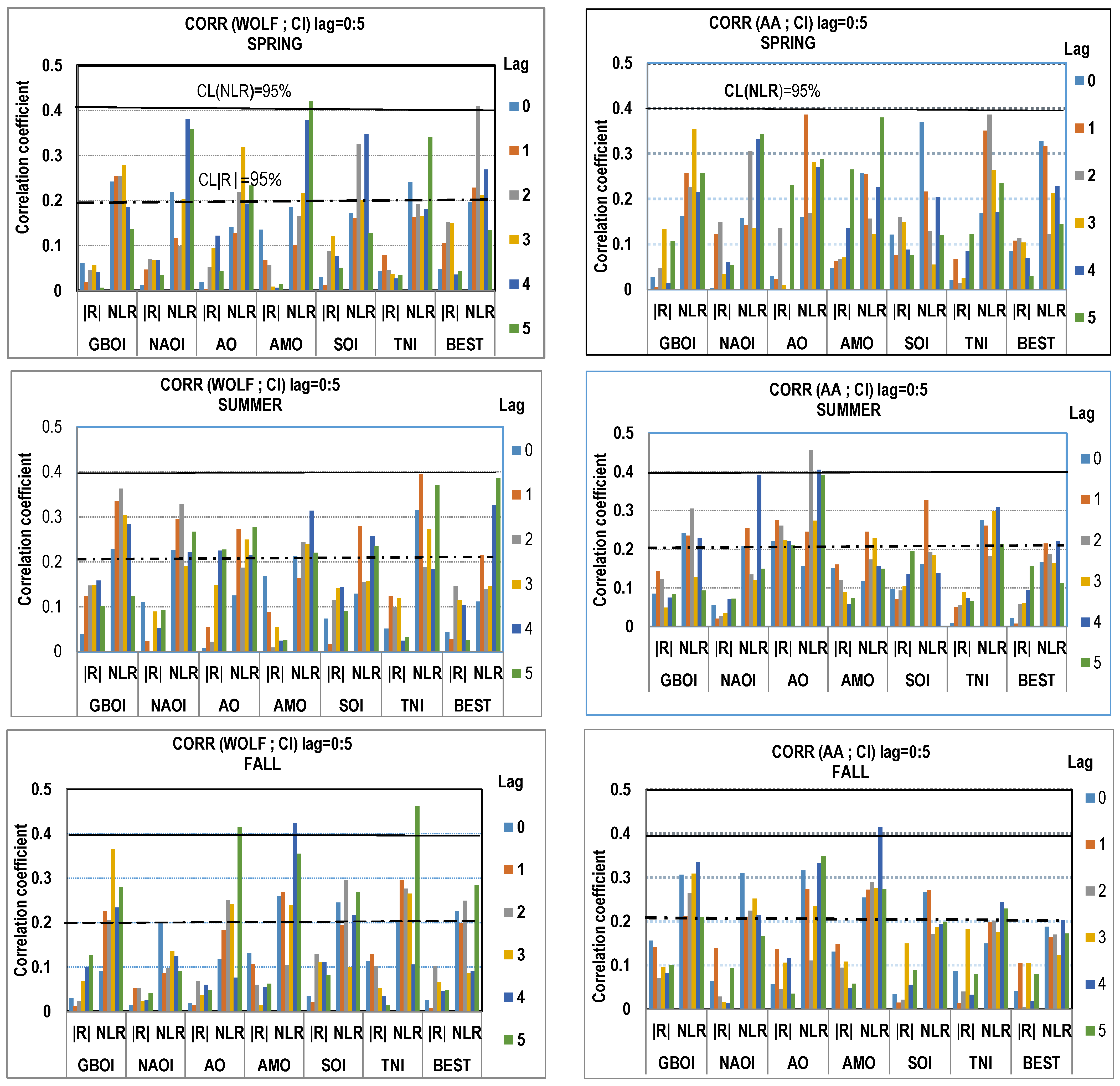
Figure 1. Pearson correlation coefficient |R| in comparison with the NLR correlation coefficient for each season and with lag from 0 to 5 years, between the Wolf number and the climate indices (left), and the aa geomagnetic index and climate indices (right). The 95% confidence level for NLR is represent with the solid lines and for R with dotted one.
Atmosphere 13 01898 g001aAtmosphere 13 01898 g001b
Figure 2. The difference between synergy and redundancy (S-R) for seven climate indices and for each season and the lags from 0 to 5 years, (left); the corresponding total correlation (TC) (right). On the y-axis are the values of the difference between synergy and redundancy (R-S).
Atmosphere 13 01898 g002aAtmosphere 13 01898 g002bAtmosphere 13 01898 g002c
Figure 3. (a) Multiple wavelet coherence (mwc) between GBOI and the two predictors aa (AA) and Wolf Number (WOLF), during winter (left panel); partial wavelet coherence (pwc) between GBOI and Wolf number, excluding the effect of aa (middle panel), and pwc between GBOI and aa, excluding the effect of Wolf number (right panel). (b) Same as (a) but for summer. The years (1901–2000) are represented on the x-axis.
Atmosphere 13 01898 g003
Figure 4. (a) Multiple wavelet coherence (mwc) between NAOI and the two predictors aa (AA) and Wolf Number (WOLF) during summer (left panel); partial wavelet coherence (pwc) between NAOI and Wolf number, excluding the effect of aa (middle panel), and pwc between NAOI and aa, excluding the effect of Wolf number (right panel). (b) Same as (a) but for winter.
Atmosphere 13 01898 g004
Figure 5. (a) Multiple wavelet coherence (mwc) between BEST and the two predictors aa (AA) and Wolf Number (WOLF) during spring (left panel); partial wavelet coherence (pwc) between BEST and Wolf number, excluding the effect of aa (middle panel), and pwc between BEST and aa, excluding the effect of Wolf number (right panel). (b) Same as (a) but for fall.
Atmosphere 13 01898 g005
Figure 6. Mwc (left panel) between summer GBOI at lag = 2, and the two predictors aa (AA) and Wolf Number (WOLF); partial wavelet coherence (pwc) between GBOI and Wolf number, excluding the effect of aa (middle panel), and pwc between GBOI and aa, excluding the effect of Wolf number (right panel).
Atmosphere 13 01898 g006
Figure 7. Mwc (left panel) between summer NAOI at lag = 2, and the two predictors aa (AA) and Wolf Number (WOLF); partial wavelet coherence (pwc) between NAOI and Wolf number, excluding the effect of aa (middle panel), and pwc between NAOI and aa, excluding the effect of Wolf number (right panel).
Atmosphere 13 01898 g007
Figure 8. Mwc (left panel) between summer NAOI at lag = 3, and the two predictors aa (AA) and Wolf Number (WOLF); partial wavelet coherence (pwc) between NAOI and Wolf number, excluding the effect of aa (middle panel), and pwc between NAOI and aa, excluding the effect of Wolf number (right panel).
Atmosphere 13 01898 g008
Figure 9. Mwc (left panel) between fall BEST at lag = 2, and the two predictors aa (AA) and Wolf Number (WOLF); partial wavelet coherence (pwc) between BEST and Wolf number, excluding the effect of aa (middle panel), and pwc between BEST and aa, excluding the effect of Wolf number (right panel).
Atmosphere 13 01898 g009
Figure 10. Left panel: Mwc between predictand (AMO) and the two predictors aa (AA) and WOLF number (WOLF) in wintertime, with lag = 4 years. Middle panel: pwc between AMO and WOLF number, eliminating the aa contribution. Right panel: pwc between AMO and aa, eliminating the Wolf number.
Atmosphere 13 01898 g010
Publisher’s Note: MDPI stays neutral with regard to jurisdictional claims in published maps and institutional affiliations.