Evaluation and Correction of Climate Simulations for the Tibetan Plateau Using the CMIP6 Models

Abstract

This study evaluates the abilities of fifteen High-resolution Coupled Model Intercomparison Project phase 6 (CMIP6) models to simulate temperature and precipitation over the Tibetan Plateau (TP) for the years 1980–2014. The impacts of terrain correction and Empirical Orthogonal Function (EOF) correction on simulations of temperature and precipitation are examined. The results show that equal-weighted ensemble averaging of the CMIP6 high-resolution model provides a good representation of the spatial distribution of temperature over the TP, although simulations underestimate observations by 1.87 °C. The simulated spatial range of temperature cooling significantly exceeds the observed range, particularly in the central and southwestern TP. The performances of the simulations for precipitation are far poorer than those for temperature, and although the CMIP6 model represents the distribution of annual mean precipitation, simulations of precipitation show significant deviations from observations. Furthermore, model simulations of precipitation are 1.57 mm lower than observed, and 30% lower than observed in the southeastern TP. However, the CMIP6 model overestimated the intensity of precipitation in most regions, especially in the southeastern part of the TP. Meanwhile, the EOF analysis indicates that the effects of the correction of temperature exceed that of precipitation. Therefore, a range of methods should be considered for correcting temperature and precipitation over a complex terrain.

1. Introduction

The Tibetan Plateau (TP) is often referred to as the “Third Pole” and “the roof of the world” [1,2,3]. Due to its high terrain, the TP is important for large-scale circulation [4]. Understanding changes to the climate over the TP has importance beyond merely understanding the immediate environment of the plateau itself [5]. Intensification of global warming has resulted in an average warming of the earth of 1.1 °C, with terrestrial temperatures rising by an average of 1.6 °C [6]. Global warming has resulted in dramatic changes to temperature and precipitation in the plateau region, which further impact the hydrological cycle [3]. Therefore, exploring the major climatic characteristics of the TP through the use of historical data is of great significance, and the knowledge gained can act as the basis for studying future climate change.

Relevant research has been limited due to the complex geographical environment over the TP, the uneven distribution of observation stations, and the limited length of data. The development of reanalysis data and climate model simulation techniques has provided a solution to these challenges. To date, global circulation models (GCMs) have been shown to have wide applicability to the TP, and have been used to detect climate change and the intensity of related atmospheric circulation [7,8,9], and to reflect the influences of local and/or large-scale atmospheric circulation processes on precipitation/temperature [10,11]. The Coupled Model Intercomparison Project (CMIP) initiated by the World Climate Research Program (WCRP) not only promotes the development and application of climate models but is also widely used in global climate change research, providing data support for the preparation of Intergovernmental Panel on Climate Change assessment reports [12,13,14]. Various studies using CMIP models have been conducted for examining evapotranspiration, heat sources, elevation-dependent warming, moisture sources, and extreme climates. In particular, past studies of the summer monsoon of the TP [15,16,17,18,19,20], showed that climate change is influencing the TP to a greater extent than other regions; for example, the rate of increase in air temperature (0.32 °C/10a from 1961 to 2010) exceeded those of national and global temperatures (0.22 °C/10a and 0.13 °C/10a), whereas precipitation is increasing, and lower sensible heat flux is decreasing [21,22,23,24,25,26].

However, model-simulation errors persist, particularly in complex terrains such as the plateau, in which model error is amplified. Zhou et al. [22] assessed abnormal warming of the TP using CMIP3 data and their results showed an opposite trend to observations. This disparity could have been related to the lack of natural forcing in the CMIP3 model. CMIP5 is an improvement on CMIP3 in that it considers different emission scenarios. Li et al. [24] used detrending analysis to show that inter-annual and inter-decadal variations in simulations of historical temperature by the CMIP5 model are relatively consistent, with a maximum temperature difference of 2.8 °C. In contrast, although the spatial distribution of simulated precipitation is consistent with observations, there are inconsistencies in rainfall depths. Su et al. [25] evaluated the abilities of 24 GCMs to simulate surface air temperature and precipitation in the area east of 90° E over the TP, revealing that the models underestimate surface air temperature and overestimated precipitation. Although CMIP6 represents a further improvement, errors in the wet and cold conditions in the precipitation simulation over the TP persist [27,28]. In addition, most models underestimate the intensity of the annual mean radiation budget as well as the cloud radiative cooling effect over the TP, and the radiation budget during the cold-warm transition period is hard to capture in CMIP6 [29].

Precipitation and temperature simulations at regional scales are highly parameter-dependent [30,31], Thus, the evaluation of CMIP performance and discussion of systematic model biases for some sensitive areas of climatic change is distinctly important. The CMIP6 model shows an improvement in temperature simulation, although a serious overestimation of precipitation still exists [28]. Determining whether HighResMIP models can realistically simulate the observed precipitation and temperature is important for assessing the reliabilities of these models for simulating further precipitation and temperature and the corresponding impacts on the regional climate. Another question is whether there is a need to bias correct these patterns. Consequently, the present study evaluates the simulations of 15 high-resolution CMIP6 models against observation data from 1980 to 2014. The results of the present study can provide a scientific basis for predicting climate change over the TP.

2. Study Area, Materials, and Method

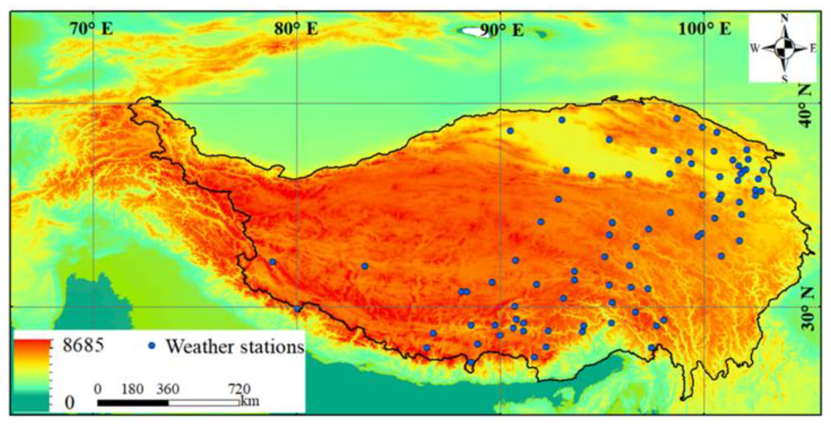
2.1. Study Area and Observational Data

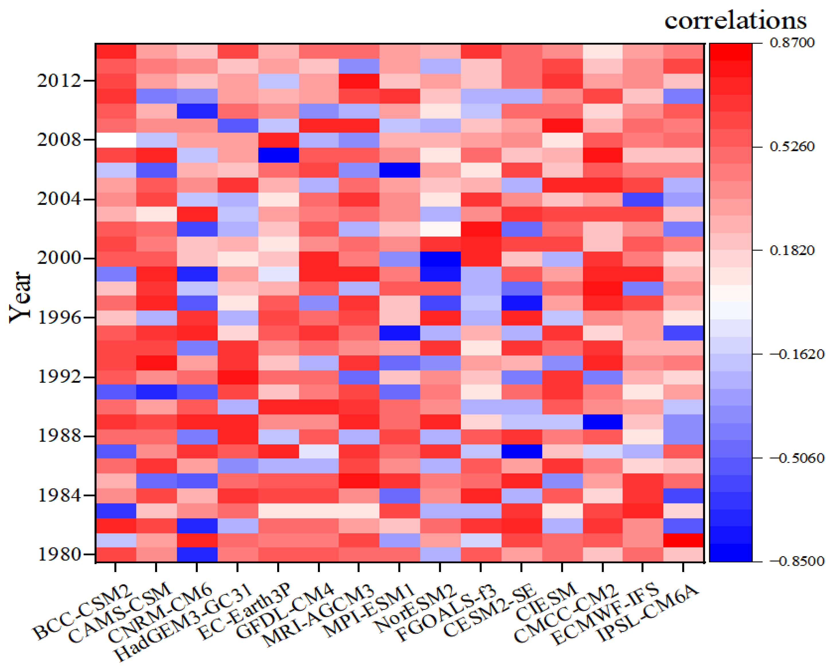
The Qinghai-Tibet Plateau region encompasses the area of 24.5°–40.5° N, 74.5°–105.5° E. Elevation in the study area decreases from the Pamir Plateau in the west (>2500 m) to the Hengduan Mountains in the east, and from the northern region of the Kunlun and Qilian Mountains in the north to the southern vein of the Himalayas in the south (Figure 1).

The present study obtains its temperature and precipitation data from daily observation records of the Tibet Autonomous Region Information Center. These data are based on a raster dataset (1980–2014) reconstructed by spline interpolation of the data from 131 surface meteorological stations, with a spatial resolution of 0.5° × 0.5°.

2.2. Model Data

The present study uses CMIP6 climate model historical simulations (https://esgf-node.llnl.gov/search/cmip6) (accessed on 15 June 2020). for 1980 to 2014, in which 1980 is chosen as a start date for evaluation as this is the beginning of the most complete set of observations on the TP. As shown in

Table 1. Models registered in CMIP6 HighResMIP.

Model	Institute	Resolution (lon × lat)
BCC-CSM2	Beijing Climate Center (China)	0.45° × 0.45°
CAMS-CSM	Chinese Academy of Meteorological Sciences, China	0.47° × 0.47°
CESM2-SE	NCAR, USA	0.9° × 1.25°
CIESM	THU/China	1.0 ° × 1.0 °
CMCC-CM2	Centro Euro-Mediterraneo sui Cambiamenti Climatici	0.25° × 0.25°
CNRM-CM6	National Centre for Meteorological Research, France	0.5° × 0.5°
EC-Earth3P	EC-Earth Consortium, Europe	0.35° × 0.35°
ECMWF-IFS	ECMWF	0.5° × 0.5°
FGOALS-f3	Chinese Academy of Sciences, China	0.25° × 0.25°
GFDL-CM4	GFDL/USA	1.0°× 1.0°
HadGEM3-GC31	Met Office Hadley Centre, UK	0.23° × 0.35°
IPSL-CM6A	IPSL	0.703° × 0.5°
MPI-ESM1	Max Planck Institute for Meteorology	0.46° × 0.46°
MRI-AGCM3	Meteorological Research Institute, Japan	0.19° × 0.19°
NorESM2	Norwegian Climate Service Centre	0.25° × 0.25°

, the present study selects data generated by 15 models, where the variant label is r1i1p1f1 and historical simulation has been completed, from the high-resolution model intercomparison program (HighResMIP) under CMIP6. Of these 15 models, the present study identifies those with a strong ability to accurately simulate the climate of the TP.

2.3. Analysis Method

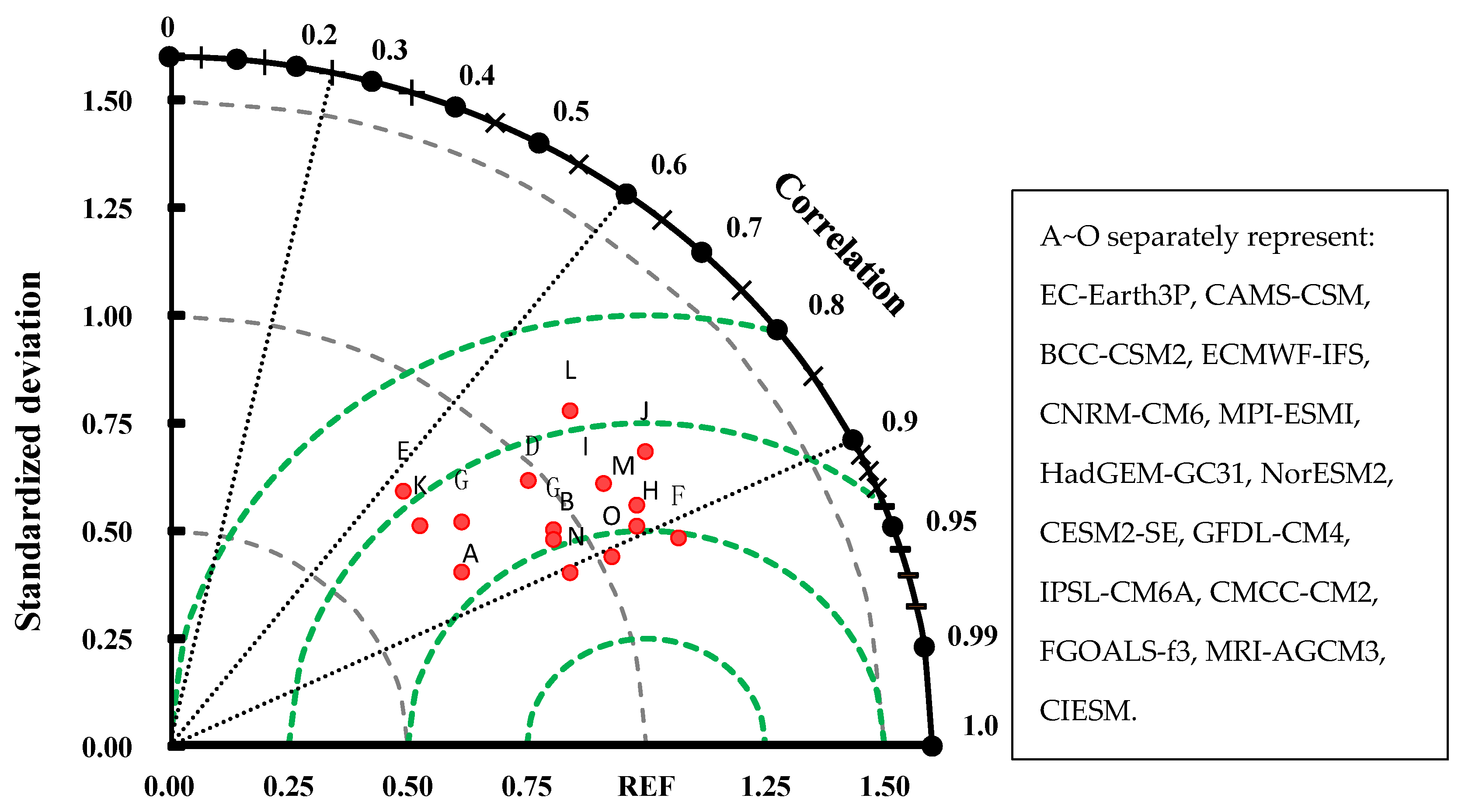
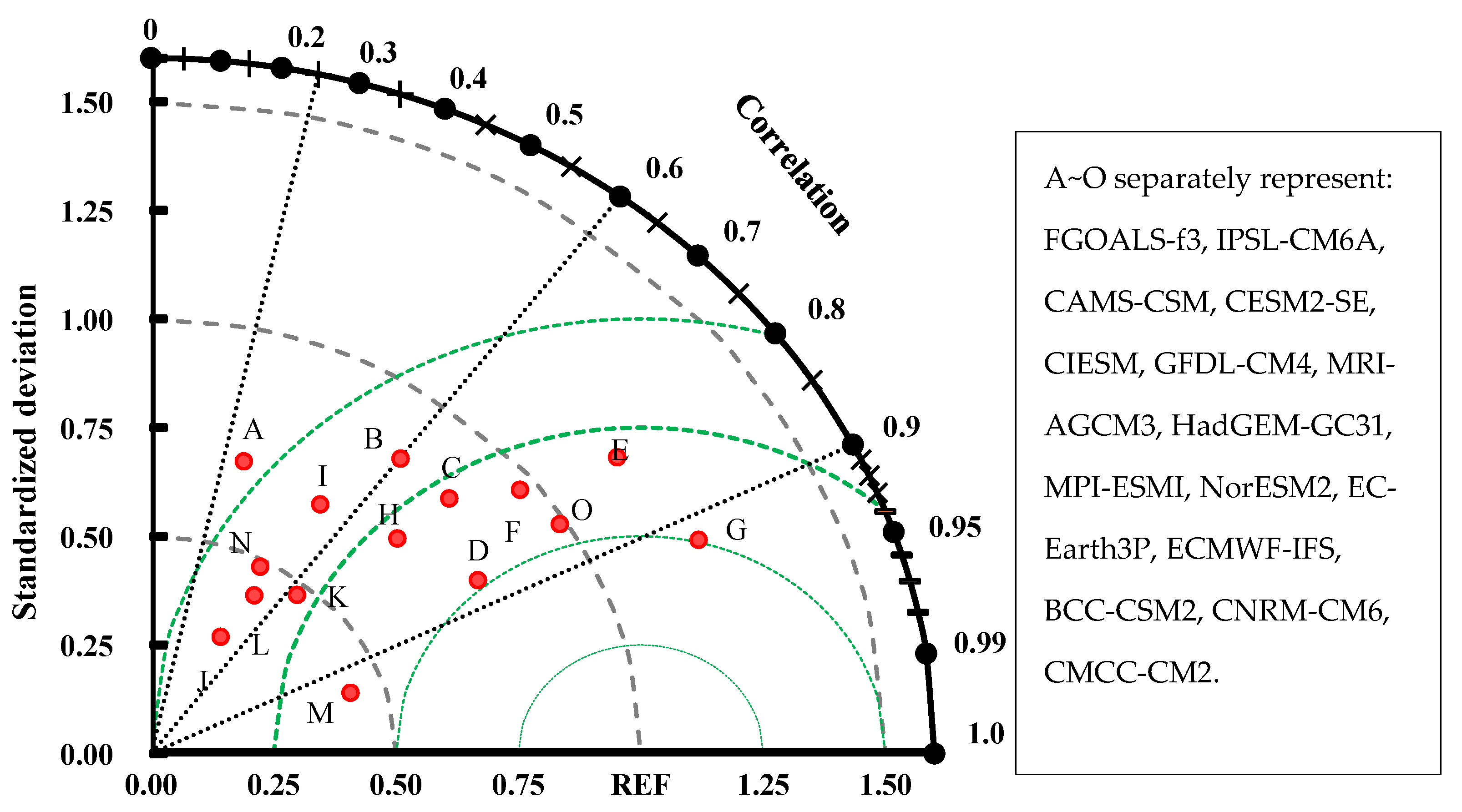
2.3.1. Taylor Diagram Method

The different models used in the present study have different spatial resolutions. Therefore, the present study first standardized the spatial resolutions of the model data to a resolution of a 0.5° × 0.5° grid through the bilinear interpolation method to facilitate comparison and subsequent data processing. The data for the area falling within China were then separated. The arithmetic averages of dimensionalities were used to obtain the annual mean temperature change for the China region from 1980 to 2014. The observed data underwent the same procedure. A comparison of model data with observed data was performed to determine the ability of the model data to approximate temperature elements in China from 1980 to 2014.

The Taylor diagram analysis method [32] allows a comparative evaluation of different GCMs by providing a graphical comparison between observations and model simulations. The method uses the ratio of standard deviations between two compared groups of sequences and the correlation coefficient to form a polar graph. This method displays the correlation coefficient, standard deviation, and centralized mean square error of the two sets of sequences on one graph, thereby providing an intuitive comparison of model simulations.

The main parameters of Taylor diagram analysis include the correlation coefficient (A_cc), the root-mean-square error (R_mse), the standard deviation of the simulated field (σ_f), and the standard deviation of observation (σ_r):

$$Acc=\frac{1}{N}{\displaystyle \sum _{n=1}^N(fn-\overline{f})(rn-\overline{r})}/\sigma f\sigma r$$

(1)

$$Rmse=\sqrt{\frac{1}{N}{\displaystyle \sum _{n=1}^N{[(fn-\overline{f})-(rn-\overline{r})]}_{}^2}}$$

(2)

$$\sigma =\sqrt{\frac{1}{N}{\displaystyle \sum _{n=1}^N{(fn-\overline{f})}_{}^2}}$$

(3)

where N represents the sample number of valid sites, and $\overline{f}$ and $\overline{r}$ are the average values of simulated and observed data, respectively.

2.3.2. EOF Error Correction

Errors in the model simulations remain after terrain correction due to parameterization errors and uncertainties in the model boundary conditions. Therefore, the present study uses the EOF method to correct the model results.

The EOF method extracts the main spatial features of observed and predicted values through EOF decomposition and establishes multiple regression equations using the time coefficients of observed and simulated fields. The details of this method are given in reference [33].

3. Results

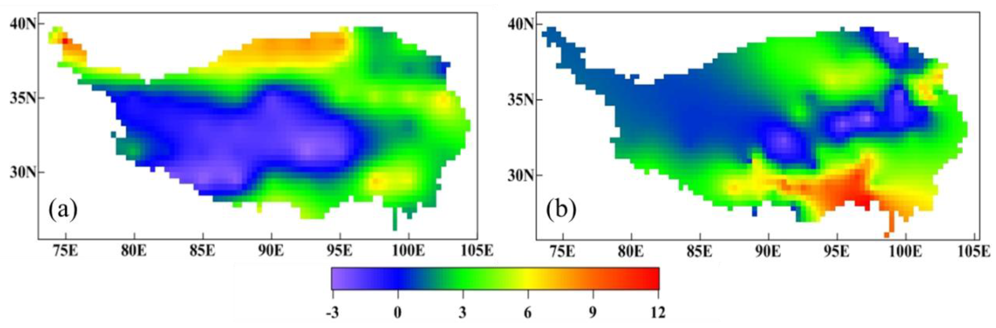
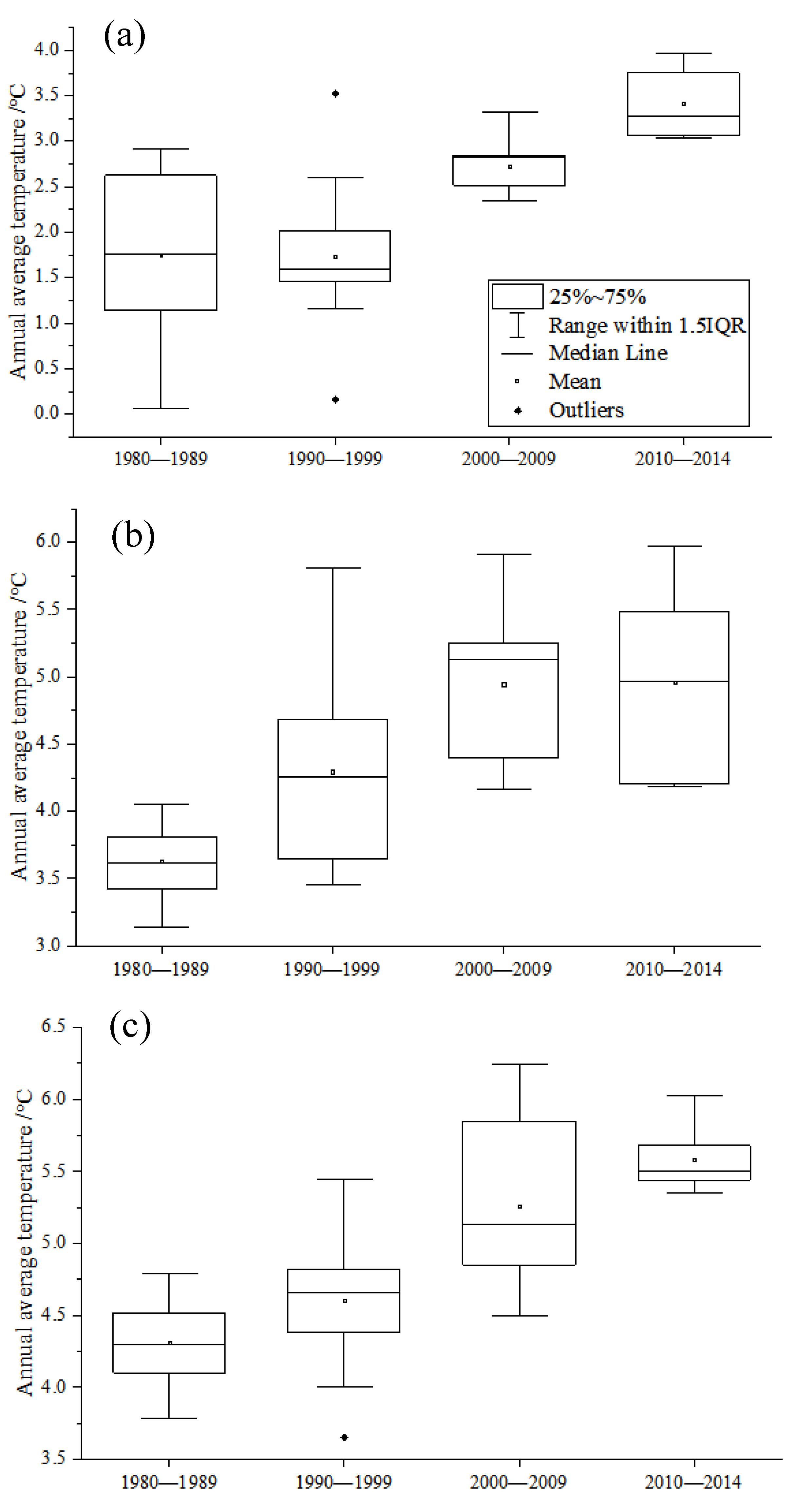
3.1. Characteristics of Temperature and Climate in the TP

Simulations of average temperature from 1980 to 2014 range from −1.6 to 6.7 °C, with an ensemble average of 2.98 °C, 1.87 °C lower than the observed value of 4.84 °C (Figure 2). The average temperatures simulated by the BCC-CSM2, CAMS-CSM, HadGEM3-GC31, MRI-AGCM3. and FGOALS-f3 models exceed the observed temperature by 1 to 2 °C. The average temperatures simulated by the GFDL-CM4, CESM2-SE, CMCC-CM2, IPSL-CM6A, and CNRM-CM6 models underestimate the observed temperature by 0.34 to 6.53 °C. The simulations of temperature by the IPSL-CM6A and CNRM-CM6 models have averages of −1.6 °C and −1.15 °C, respectively, underestimating the observed average temperature by over 5 °C. This result indicates that the two models generally underestimate temperature over the TP. The averages of temperature simulations of the EC-Earth3P, MPI-ESM1, NorESM2, and CIESM models are closest to the observed temperature among the evaluated models at 4.5, 4.43, and 4.54 °C, respectively. Hu et al. [34] used 44 CMIP5 models to simulate the surface air temperature over the TP. Their study found a deviation in temperature simulations among the models of −6.2 °C to 1.8 °C, with CNRM-CM5 underestimating temperature by 6.2 °C and three models underestimating the observed temperature by over 5 °C. A study by Zhu et al. [28] using CMIP6 models to simulate air temperature over the TP revealed a variation in temperature simulations of −7.4 °C to 3.1 °C in temperature simulation among the 23 models. The average of the temperature simulations by the IPSL-CM6A model deviated from temperature observations by over 3 °C, consistent with the results of the present study. Past studies have shown that most of the CMIP6 models perform badly in simulating the average temperature over the TP, with the CNRM-CM6 and IPSL-CM6A models showing the worst performance.

The equal-weighted ensemble average of the CMIP6 model simulations provides an improved representation of the observed spatial distribution of temperature over the TP, although the model simulations underestimate observations (Figure 3). The spatial range of the equal-weighted ensemble average simulated temperature cooling far exceeds the observed temperature cooling, particularly in the central and southwestern parts of the TP. The averages of model-simulated temperatures for Puran and Nyalam are negative, whereas observed values are positive. In addition, model simulations indicate that the areas with higher temperatures are in the north and northwest, whereas the colder areas are in the east and southeast, a spatial pattern opposite to that of the observed data. Areas of higher observed temperature are in the south to southeastern parts of Tibet encompassing the eastern part of the Himalayas, with a relatively low altitude. However, the model simulations fail to represent this spatial pattern in air temperature. Model simulations also overestimate the temperatures of the high-altitude Pamir region, possibly related to incorrect pattern interpolation.

The CMIP6 models show some improvement in simulating global and Chinese overall mean and extreme temperature and precipitation compared to other models, both in China and globally [28,35,36]. However, Figure 3a shows low temperature is more obvious in the western part of the TP, which may be related to the area of snow cover. Snow and ice cover lead to higher albedo, and a physically interrelated process exists between albedo and cold bias [37]. Different parameterizations of snow cover in most GCMs lead to different albedos. In addition, the deviation in the simulation of cloud physical processes [38], ground heat sources [26], and greenhouse gases [39] will also lead to the cold bias of the TP.

The present study used the observed data to calculate the average temperature over the TP. The results showed an increase in temperature from 1980 to 2014 at a rate of 0.43 °C/10a. Correlations between the model simulations and observations from 1980 to 2014 were calculated to better understand the ability of the models to simulate the overall trend in air temperature over the TP (Figure 4). Among the models, the simulations of MPI-ESM1 showed the highest correlation to the observed data, indicating that this model most accurately captured the overall trend in the observed data. In the analysis, MPI-ESM1 obtained the highest correlation coefficient (0.73), whereas that between HadGEM3-GC31 and NorESM2 was ~0.65. In general, the models showed poor performances in simulating the overall trend in average temperature over the Tibetan Plateau. CNRM-CM6 obtained the lowest correlation coefficient of 0.32, whereas those of the remaining models ranged between 0.47–0.6. The period showing the highest rate of temperature increase of 0.27 °C/10a was 1998–2013. The results showed that the simulations of all models were highly correlated with the observed data during this period, indicating that most model simulations also show a warming trend during this period. The simulations of EC-Earth3P were closest to the observations during this period (96%). The simulation performances of all models were poor on a year-to-year basis, particularly for years of abrupt climate change, such as during the late 1980s and early 2000s, during which the simulations of some models showed opposite trends to the observations.

All models showed a good performance in simulating changes in temperature over time, with relatively small errors. The optimal way of selecting a model is to assess model performances across many simulation elements. Additionally, the results showed that models with poor simulation performance had a relatively low atmospheric resolution, indicating that the atmospheric resolution of a model affects its simulation accuracy. The description of atmospheric physical processes in the model is very important. The difference in description results in the difference in the simulation ability of meteorological elements between the models, and the impact is greater than that of the model resolution.

A Taylor diagram is used to further evaluate the simulation performance of each model. As shown in Figure 5, correlation coefficients between simulated annual average temperature and observations among the evaluated models range from 0.4 to 0.7. The highest and lowest correlations are obtained by the MPI-ESMI and CNRM-CM6, models, respectively. Furthermore, the correlation coefficients of five models are below 0.8 for the TP, whereas most models show higher correlation coefficients. This result indicates that the models performed relatively well in representing the observed spatial variability in annual average temperature over the TP. Within the model evaluations, the ratios of standard deviations between model simulations and observations range from 0.7 to 1.25. Among the models, MRI-AGCM3, CIESM, and NorESM2 show good performances in simulating the spatial distribution of air temperature, with root mean square errors ranging from 0.5 to 0.75. The EC-Earth3P model provides the most accurate simulation of air temperature (Figure 4 and Figure 5), and the FGOALS-f3 model underestimates the inter-annual variability in the analogs, whereas the remaining models overestimate the inter-annual variability in the analogs (Figure 4 and Figure 5). A comparison of the simulations of 23 CMIP6 models with an observational dataset (CN05.1) for the period 1961–2014 by Zhu et al. [28] found that the IPSL-CM6A-LR, CanESM5, FGOALS-g3, SAM0-UNICON, E3SM-1-0, and NorESM2-LM showed larger biases (over 3 °C).

Corrections to deviations are recommended in the case of small model deviations and limited observed data. Short-term simulations show relatively small deviations, and any change in the model will require historical predictions to be repeated. Therefore, corrections to deviations are rarely performed for short-term simulations, whereas they are required for long-term simulations to avoid model drift.

The Empirical Orthogonal Function (EOF) and Single Value Decomposition (SVD) methods were used to correct inter-seasonal prediction errors in the East Asian summer monsoon model. Although their results showed that the two methods have similar effects, the EOF provides better corrections of anomalies in precipitation intensity [33].

As shown in Figure 6, the corrected simulations significantly exceed the average of the original model ensemble by 1–3 °C, with averages of the corrected simulations and original simulations of 4.38 °C and 2.98 °C, respectively (Figure 6a,b). The corrected simulations are within ±1 °C of the observations (average of 4.8 °C) (Figure 6c). The EOF-corrected simulations for 1999 to 2001 and 2003, 2005, 2008, and 2011 still overestimate the temperature by 0.2–0.5 °C, although there is no difference between the corrected simulations and original simulations for 2013. Although the EOF correction on average increases the simulated predictions of temperature, the simulations continue to underestimate or overestimate temperature, indicating that other uncertainties are affecting the model simulations.

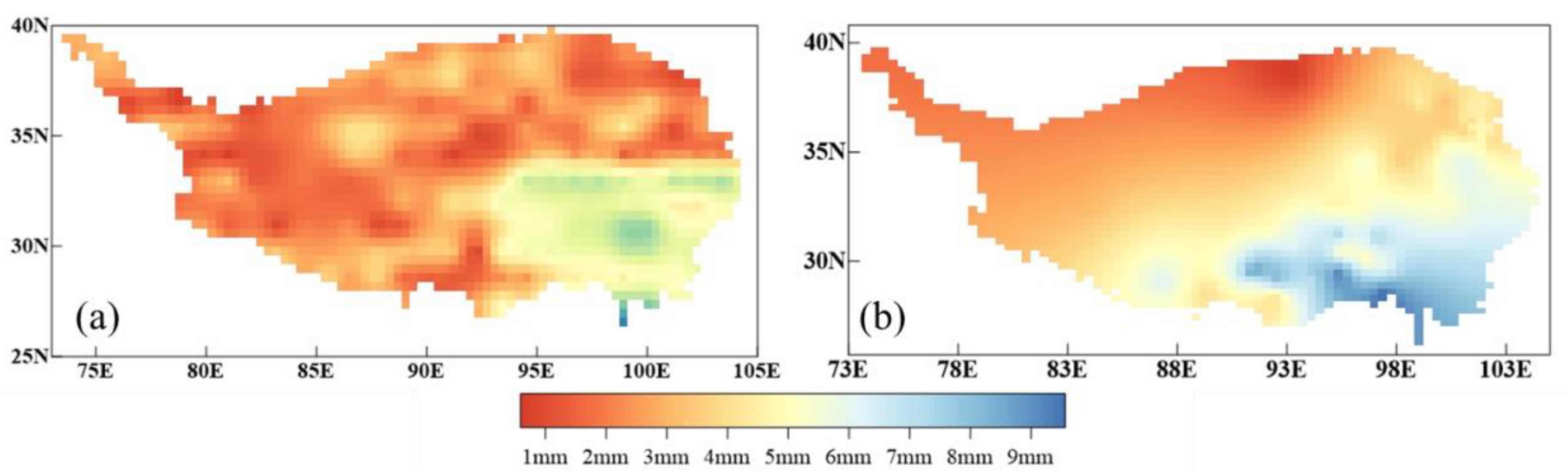
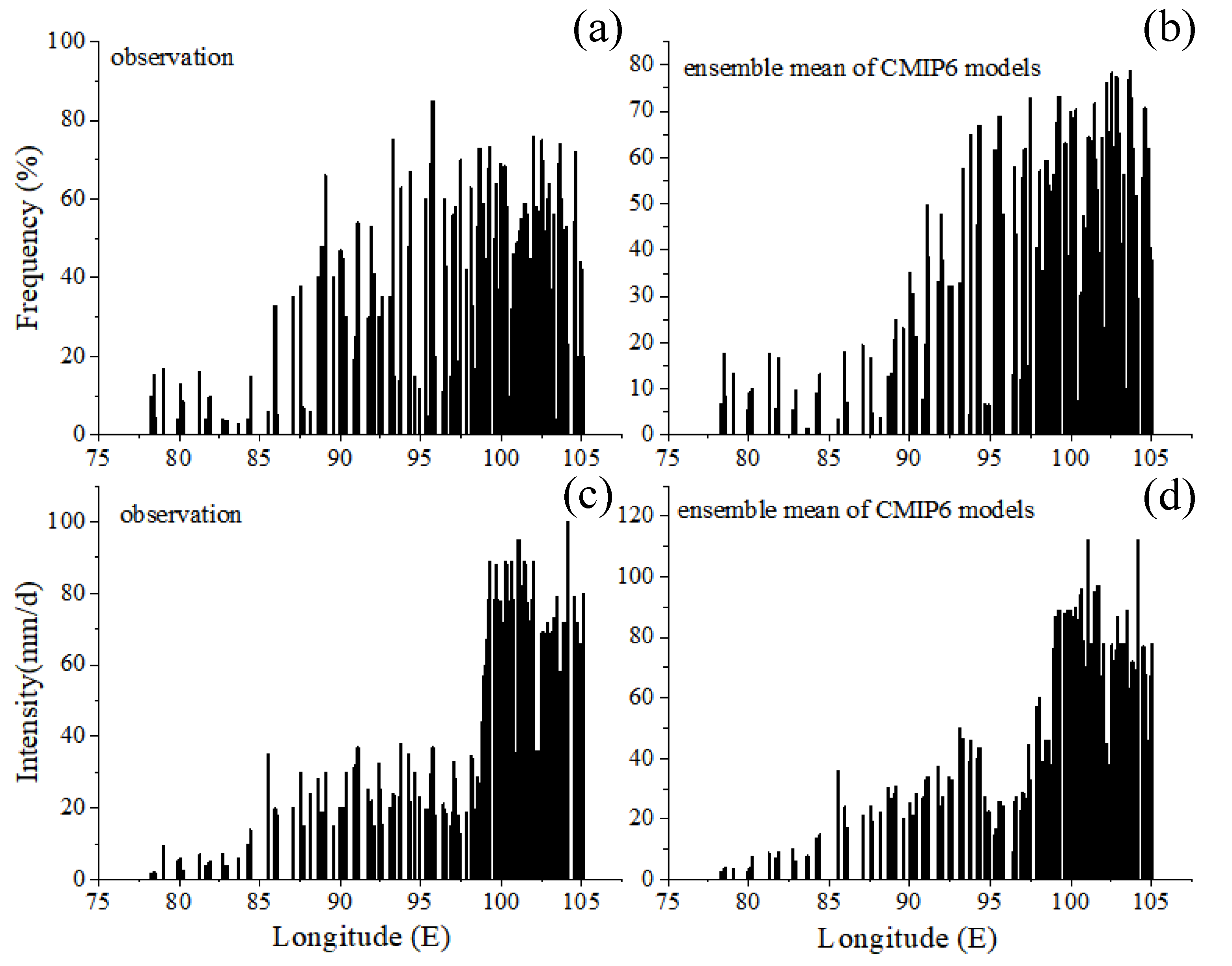
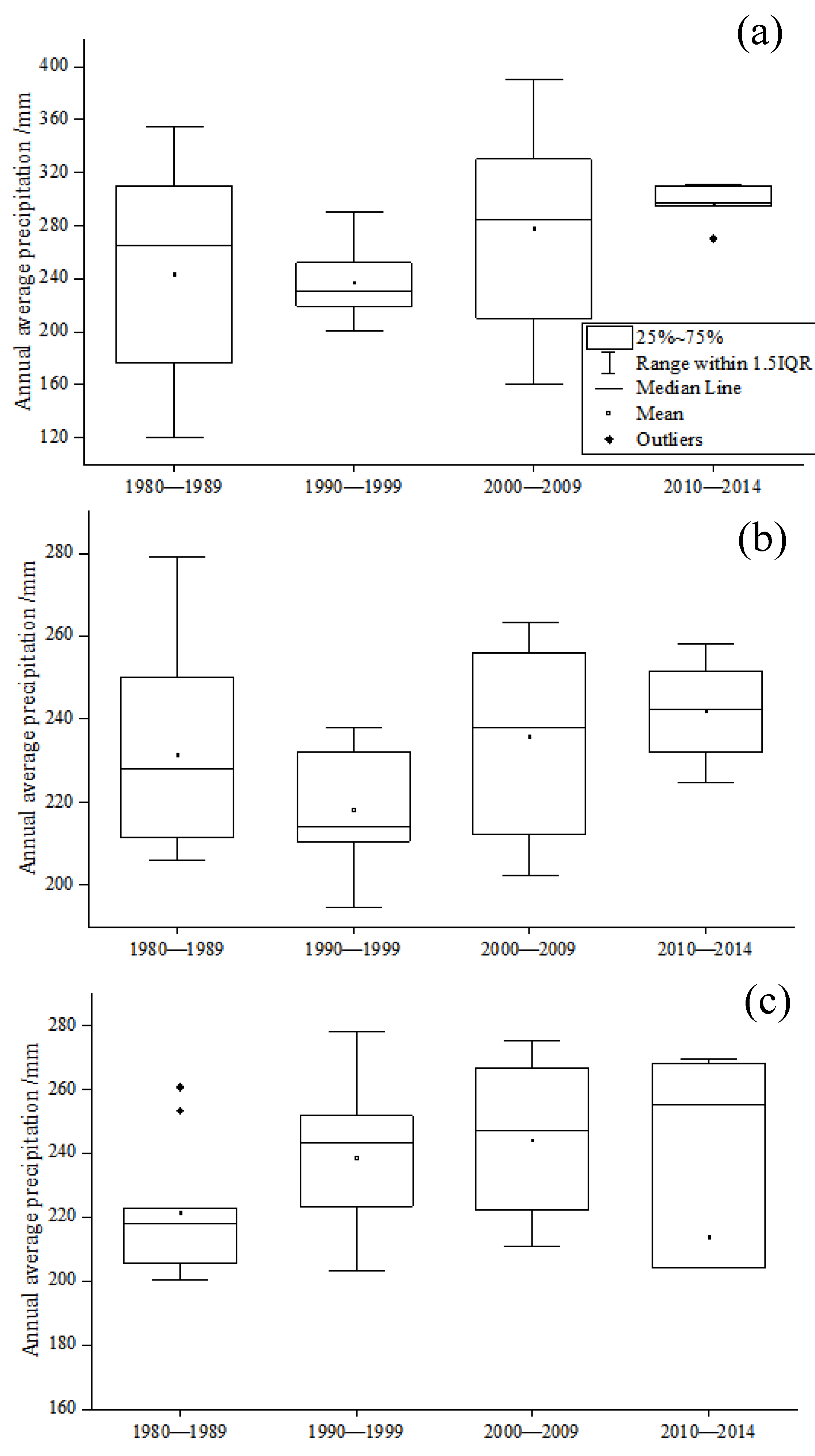
3.2. Characteristics of Precipitation in the TP

The observed precipitation data for the TP shows a decreasing trend in precipitation from southeast to northwest (Figure 7a). The average simulations of precipitation by the CMIP6 model ensemble reproduce the observed spatial distribution of precipitation (Figure 7b). The model ensemble average results reproduced the gradient distribution of precipitation from southeast to northwest of the plateau, capturing the higher precipitation zone in the south. However, the model simulations overestimated precipitation in the southeast, with a false area of high precipitation on the eastern slope of the plateau. The model simulations precipitation compared to the observed varied by 1.57 mm (30%) in the southeast and by 60–75% in Lhasa and Shigaze. These results indicate that the models still show limitations in simulating precipitation. The results of the present study are consistent with those of Hu et al. [40]. The increase in the spatial resolution of the EC-Earth3P model for the TP reduces variations in simulated precipitation, particularly along the northern and southern margins, with that in the east to less than 25%.

The mean precipitation can be further decomposed into precipitation frequency and intensity, and different combinations of frequency and intensity may exhibit similar precipitation climatic characteristics. Both the frequency and intensity of precipitation simulations need to be assessed to further reveal the model simulation deviations from the observed data [16,41]. The spatial variations in simulated precipitation frequency were similar to that of precipitation (Figure 8a,c). The observed precipitation indicated that the southern edge and southeast of the plateau are among the steep terrain regions in which precipitation occurs most frequently, with a frequency of up to 48.7%. In common with the precipitation spatial distribution, the frequency of precipitation varies spatially. The southeast portion of the plateau receives the most precipitation, with a precipitation frequency that can exceed 40%. Precipitation exceeding 5 mm/d is mainly concentrated within 85° and 105° E. Around 1% of days show a precipitation intensity >25 mm/d, mainly concentrated within 100° and 105° E. The southeastern corner of the plateau’s low-altitude region experiences precipitation at a rate that is noticeably higher than that of the high-altitude region, with a maximum precipitation intensity that can exceed 100 mm/d (mainly in the Milin and Metuo areas of Nyingchi). Precipitation intensity increases from the interior of the plateau to the southeast and the CMIP6 high-resolution model generally reproduced observed higher frequency precipitation. However, the results show that the precipitation intensity of the model (52.98 mm/d) was greater than the observed precipitation intensity (43.78 mm/d) in most regions, while the precipitation frequency of the model (25.29%) was close to the observed precipitation frequency (25.60%). (Figure 8b,d). The precipitation simulations of GFDL-CM4 showed a spatial distribution of precipitation intensity that was closest to observed. The simulations of BCC-CSM2, FGOALS-f3, and HadGEM3-GC31 showed the highest frequencies of precipitation exceeding 25 mm/d, whereas CNRM-CM6 showed the lowest. The remaining models, notably ECMWF-IFS, EC-Earth3P, and MPI-ESM1, generated far smaller frequencies of precipitation (picture omitted).

Previous studies have shown that model simulations of precipitation in the south and southeast area of the TP exceed observations, particularly for the CMIP6, CMIP3, and CMIP5 models [42,43]. However, this overestimation in precipitation has been somewhat reduced due to improvements in the CMIP6 model in capturing the convergence characteristics of meridional water vapor flux, thereby reducing errors in simulations of the meridional and zonal specific humidity vortices [35,44]. In addition, the precipitation processes over the TP are extremely complex and are not only affected by local convective processes and large-scale circulation, but also by topography [45,46,47]. Although topographic correction has improved the simulations of precipitation, it can only change precipitation in topographically affected areas by 20.2% [48,49]. Therefore, the overestimation of precipitation will persist within modeling studies. In addition, the water vapor source of precipitation over the TP may be related to westerlies and monsoons [18,50,51,52]. Duan et al. [53] also emphasized the indirect effect of sulfate aerosols in improving the ability of the model to simulate the annual precipitation cycle, although significant deviation persists.

The Taylor diagram analysis of each model results in mixed results, with correlation coefficients and standard deviation between simulations and observations among each model ranging from 0.2 to 0.9 and 0.2 to 1.2, respectively (Figure 9). The dispersed distribution of results of the 15 models of the TP indicated that the models differ widely in their ability to reproduce the spatial variations in precipitation climatology. Furthermore, the correlation coefficients of the five models were below 0.60 for the TP, whereas most of the models show higher correlation coefficients. The simulations of the MRI-AGCM3, BCC-CSM2, and CNRM-CM6 models show the lowest ratio of standard deviations and highest correlation coefficients (over 0.5) with observations. The correlation coefficients of FGOALS-f3, NorESM2, and CNRM-CM6 fail to exceed 0.5, and the standard deviations of the simulations of these models are also significantly different from that of the observed data. This result further emphasizes the limitations of the models for simulating precipitation.

The abilities of the models to simulate the annual average precipitation over the TP are generally poorer compared to that of air temperature, despite the models performing well in representing the spatial distribution and intensity of the precipitation. Several CMIP6 models still perform poorly in simulating annual average precipitation over the TP. One of the main factors affecting the performance of regional-scale precipitation simulation is the horizontal resolution of a model. The horizontal resolutions of most models are insufficiently high to resolve the important processes and features affecting the region. Many physical mechanisms are involved in the simulation of diurnal precipitation variation within climate models and simulations may be impacted by changes in the convective parameterization scheme and the radiative transport scheme. The regional distributions of precipitation frequency and intensity can be closely replicated by the various CMIP6 GCMs. However, the models overestimate and underestimate precipitation frequency and intensity over the TP, respectively. The simulations of precipitation for the southern and eastern slopes of the plateau continue to show substantial deviation from observations, despite the fact that the improvement in model resolution reduces simulation bias.

EOF correction is further performed on the model simulations of precipitation. As shown in Figure 10, corrected simulations of annual precipitation exceed the observations by 6.7 mm. The overall performance of corrected precipitation is poor compared with that of temperature, indicating that the different correction methods have regional advantages: methods suitable for temperature correction for a particular region may not be effective for precipitation correction. Since the correction of precipitation is more complex than that of temperature, a combination of various correction methods can be considered for the correction of precipitation in complex terrain.

4. Conclusions

Although the CMIP6 model is now better able to predict precipitation over the TP, the issue of systematic divergence in areas of steep terrain persists. The TP’s topography is complicated and highly varying, and the high topography of the plateau and that of its neighboring areas have a significant impact on the region’s precipitation patterns. The present study assessed the bias of the current model through a methodical evaluation of model simulation results. However, further investigation is required to understand the uncertainty in model simulations.

The current study evaluates the performances of CMIP6 high-resolution models in representing historical observed air temperature and precipitation over the TP. Moreover, the improvements of model simulations through terrain and EOF correction are evaluated.

While the equal-weighted ensemble averages of CMIP6 high-resolution model simulations of temperature are representative of the observed spatial distribution of temperature on the TP, they, on average, underestimate temperature by 1.87 °C. Most models are able to depict an increase in mean temperature across the Qinghai-Tibet Plateau between 1981 and 2014, which is a reasonable simulation of the general trends in mean temperature change over the TP. The simulations of annual average temperature by some models are close to observations. The spatial range of temperature cooling of the model simulations exceeds that of the observed data. The model simulations overestimate the spatial range of low temperatures over the central and southwestern TP. The models show poor performance in representing the overall trend in average temperature over the TP, particularly during years of abrupt climate change, with the simulations of some models negatively correlated with the observed results.

The performances of the CMIP6 models for simulating precipitation over the TP are clearly poorer than for temperature. While the models are able to represent the spatial distribution of observed annual mean precipitation, simulations of precipitation depth show significant deviations from the observed rainfall. Model simulations of precipitation underestimate observations by 1.57 mm, and by 30% in the southeast. Most models overestimated the intensity of precipitation, mainly in the southeast, low-altitude region of the plateau.

EOF correction of simulations of TP temperature is more effective than EOF correction of precipitation, indicating the feasibility and effectiveness of this method. However, it should also be noted that the revised precipitation model can still be improved. This result indicates that a variety of correction methods can be considered when correcting temperature and precipitation over a complex terrain.

References

1. Kang, S.C.; Xu, Y.W.; You, Q.L.; Flugel, W.A.; Pepin, N.; Yao, T.D. Review of climate and cryospheric change in the Tibetan Plateau. Environ. Res. Lett. 2010, 5, 015101. [Google Scholar] [CrossRef]
2. Kang, S.C.; Zhang, Q.G.; Qian, Y.; Ji, Z.M.; Li, X.L.; Cong, Z.Y.; Zhang, Y.L.; Guo, J.M.; Du, W.T.; Huang, J.; et al. Linking atmospheric pollution to cryospheric change in the Third Pole region: Current progress and future prospects. Natl. Sci. Rev. 2019, 6, 796–809. [Google Scholar] [CrossRef] [PubMed]
3. Yao, T.D.; Xue, Y.K.; Chen, D.L.; Chen, F.H.; Thompson, L.; Cui, P.; Koike, T.K.-M.; Lau, W.; Lettenmaier, D.; Mosbrugger, V.; et al. Recent Third Pole’s rapid warming accompanies cryospheric melt and water cycle intensification and interactions between monsoon and environment: Multi-disciplinary approach with observation, modeling and analysis. Bull. Am. Meteorol. Soc. 2019, 100, 423–444. [Google Scholar] [CrossRef]
4. Liu, S.F.; Duan, A.M.; Wu, G.X. Asymmetrical response of the East Asian summer monsoon to the quadrennial oscillation of global sea surface temperature associated with the Tibetan Plateau thermal feedback. J. Geophys. Res. Atmos. 2020, 125, e2019JD032129. [Google Scholar] [CrossRef]
5. Zhang, G.Q.; Yao, T.D.; Xie, H.J.; Yang, K.; Zhu, L.P.; Shum, C.K.; Bolch, T.; Yi, S.; Allen, S.; Jiang, L.G. Response of Tibetan Plateau lakes to climate change: Trends, patterns, and mechanisms. Earth Sci. Rev. 2020, 208, 103. [Google Scholar] [CrossRef]
6. Zhai, V.P.; Pirani, A.; Connors, S.L.; Péan, C.; Berger, S.; Caud, N.; Chen, Y.; Goldfarb, L.; Gomis, M.I.; Huang, M.; et al. (Eds.) Climate Change 2021: The Physical Science Basis. Contribution of Working Group I to the Sixth Assessment Report of the Intergovernmental Panel on Climate Change; Cambridge University Press: Cambridge, UK, 2021. [Google Scholar]
7. Grotch, S.L.; MacCracken, M.C. The Use of General Circulation Models to Predict Regional Climatic Change. J. Clim. 1991, 4, 286–303. [Google Scholar] [CrossRef]
8. Shepherd, T. Atmospheric circulation as a source of uncertainty in climate change projections. Nat. Geosci. 2014, 7, 703–708. [Google Scholar] [CrossRef] [Green Version]
9. Peshev, Z.; Deleva, A.; Vulkova, L.; Dreischuh, T. Large-Scale Saharan Dust Episode in April 2019: Study of Desert Aerosol Loads over Sofia, Bulgaria, Using Remote Sensing, In Situ, and Modeling Resources. Atmospheric 2022, 13, 981. [Google Scholar] [CrossRef]
10. Angeles, M.E.; Gonzalez, J.E.; Erickson III, D.J.; Hernández, J.L. Predictions of future climate change in the caribbean region using global general circulation models. Int. J. Climatol. 2007, 27, 555–569. [Google Scholar] [CrossRef]
11. Smith, D.M.; Eade, R.; Andrews, M.B.; Ayres, H.; Clark, A.; Chripko, S.; Deser, C.; Dunstone, N.J.; García-Serrano, J.; Gastineau, G.; et al. Robust but weak winter atmospheric circulation response to future Arctic sea ice loss. Nat. Commun. 2022, 13, 727. [Google Scholar] [CrossRef]
12. Amjad, M.; Yilmaz, M.T.; Yucel, I.; Yilmazb, K.K. Performance Evaluation of Satellite- and Model-based Precipitation Products over Varying Climate and Complex Topography. J. Hydrol. 2020, 584, 124707. [Google Scholar] [CrossRef]
13. Zhou, T.J.; Zou, L.W.; Chen, X.L. Commentary on the Coupled Model Intercomparison Project Phase 6 (CMIP6). Adv. Clim. Chang. Res. 2019, 15, 445–456. (In Chinese) [Google Scholar] [CrossRef]
14. Wang, X.J.; Pang, G.J.; Yang, M.X. Precipitation over the Tibetan Plateau during recent decades: A review based on observations and simulations. Int. J. Climatol. 2018, 38, 1116–1131. [Google Scholar] [CrossRef]
15. Zhang, X.T.; Wang, L.; Chen, D.L. How does temporal trend of reference evapotranspiration over the Tibetan Plateau change with elevation? Int. J. Climatol. 2019, 39, 2295–2305. [Google Scholar] [CrossRef]
16. Li, J.; Yu, R.C.; Yuan, W.H.; Chen, H.M.; Sun, W.; Zhang, Y. Precipitation over East Asia simulated by NCAR CAM5 at different horizontal resolutions. J. Adv. Model. Earth. Syst. 2015, 7, 774–790. [Google Scholar] [CrossRef]
17. Wang, Z.Z.; Zhan, C.S.; Ning, L.K.; Guo, H. Evaluation of global terrestrial evapotranspiration in CMIP6 models. Theor. Appl. Climatol. 2021, 143, 521–531. [Google Scholar] [CrossRef]
18. Shang, W.; Duan, K.Q.; Li, S.S.; Ren, X.J.; Huang, B. Simulation of the dipole pattern of summer precipitation over the Tibetan Plateau by CMIP6 models. Environ. Res. Lett. 2021, 16, 014047. [Google Scholar] [CrossRef]
19. Zhang, G.W.; Zeng, G.; Yang, X.Y.; Jiang, Z.H. Future Changes in Extreme High Temperature over China at 1.5 ℃–5 ℃ Global Warming Based on CMIP6 Simulations. Adv. Atmos. Sci. 2021, 38, 253–267. [Google Scholar] [CrossRef]
20. Salunke, P.; Jain, S.; Mishra, S.K. Performance of the CMIP5 models in the simulation of the Himalaya-Tibetan Plateau monsoon. Theor. Appl. Climatol. 2019, 137, 909–928. [Google Scholar] [CrossRef]
21. Hu, T.; Sun, Y. Anthropogenic influence on extreme temperatures in China based on CMIP6 models. Int. J. Climatol. 2022, 42, 2981–2995. [Google Scholar] [CrossRef]
22. Zhou, T.J.; Yu, R.C. Twentieth-century surface air temperature over China and the globe simulated by coupled climate models. J. Clim. 2006, 19, 5843–5858. [Google Scholar] [CrossRef]
23. You, Q.L.; Jiang, Z.H.; Wang, D.; Pepin, N.; Kang, S.C. Simulation of temperature extremes in the Tibetan Plateau from CMIP5 models and comparison with gridded observations. Clim. Dyn. 2018, 27, 355–369. [Google Scholar] [CrossRef] [Green Version]
24. Li, Z.C.; Wei, Z.G.; Lv, S.H.; Gao, Y.H.; Han, B.; Li, S.S.; Ao, Y.H.; Chen, H. Verifications of surface air temperature and precipitation from CMIP5 model in northern hemisphere and Qinghai-Xizang Plateau. Plateau Meteorol. 2013, 32, 921–928. (In Chinese) [Google Scholar]
25. Su, F.G.; Duan, X.L.; Chen, D.L.; Hao, Z.C.; Cuo, L. Evaluation of the global climate models in the CMIP5 over the Tibetan Plateau. J. Clim. 2013, 26, 3187–3208. [Google Scholar] [CrossRef] [Green Version]
26. Wang, M.R.; Zhou, S.W.; Sun, Y.; Wang, J.; Ma, S.J.; Yu, Z.S. Assessment of the Spring Sensible Heat Flux over the Central and Eastern Tibetan Plateau Simulated by CMIP6 Multi-models. Chin. J. Atmos. Sci. 2022, 46, 1225–1238. (In Chinese) [Google Scholar] [CrossRef]
27. Hu, Q.; Hua, W.; Yang, K.Q.; Ming, J.; Ma, P.; Zhao, Y.; Fan, G.Z. An assessment of temperature simulations by CMIP6 climate models over the Tibetan Plateau and differences with CMIP5 climate models. Theor. Appl. Climatol. 2022, 148, 223–236. [Google Scholar] [CrossRef]
28. Zhu, Y.Y.; Yang, S.N. Evaluation of CMIP6 for historical temperature and precipitation over the Tibetan Plateau and its comparison with CMIP5. Adv. Clim. Chang. Res. 2020, 11, 239–251. [Google Scholar] [CrossRef]
29. Li, J.D.; Sun, Z.A.; Liu, Y.M.; You, Q.L.; Chen, G.X.; Bao, Q. Top-of-Atmosphere Radiation Budget and Cloud Radiative Effects Over the Tibetan Plateau and Adjacent Monsoon Regions From CMIP6 Simulations. J. Geophys. Res. 2021, 126, e2020JD034345. [Google Scholar] [CrossRef]
30. Ji, D.; Dong, W.J.; Hong, T.; Dai, T.L.; Zheng, Z.Y.; Yang, S.L.; Zhu, X. Assessing parameter importance of the weather research and forecasting model based on global sensitivity analysis methods. J. Geophys. Res. Atmos. 2018, 123, 4443e4460. [Google Scholar] [CrossRef]
31. Neelin, J.D.; Bracco, A.; Luo, H.; Meyerson, J.E.; Affiliation, A.I. Considerations for parameter optimization and sensitivity in climate models. Proc. Natl. Acad. Sci. USA 2010, 107, 21349e21354. [Google Scholar] [CrossRef] [Green Version]
32. Taylor, K.E. Summarizing multiple aspects of model performance in a single diagram. J. Geophys. Res. 2001, 106, 7183–7192. [Google Scholar] [CrossRef]
33. Li, F.; Lin, Z.D.; Zuo, R.T.; Zeng, Q.C. The Methods for Correcting the Summer Precipitation Anomaly Predicted Extraseasonally over East Asian Monsoon Region Based on EOF and SVD. Clim. Environ. Res. 2015, 11, 658–668. (In Chinese) [Google Scholar] [CrossRef]
34. Hu, Q.; Jiang, D.B.; Fan, G.Z. Evaluation of CMIP5 models over the Qinghai-Tibetan Plateau. Chin. J. Atmos. Sci. 2014, 38, 924–938. (In Chinese) [Google Scholar] [CrossRef]
35. Dong, T.Y.; Dong, W.J. Evaluation of extreme precipitation over Asia in CMIP6 models. Clim. Dyn. 2021, 57, 1751–1769. [Google Scholar] [CrossRef]
36. Lun, Y.R.; Liu, L.; Cheng, L.; Li, X.P.; Li, H.; Xu, Z.X. Assessment of GCMs simulation performance for precipitation and temperature from CMIP5 to CMIP6 over the Tibetan Plateau. Int. J. Climatol. 2021, 41, 3994–4018. [Google Scholar] [CrossRef]
37. Chen, X.; Liu, Y.; Wu, G.X. Understanding the surface temperature cold bias in CMIP5 AGCMs over the Tibetan Plateau. Adv. Atmos. Sci. 2017, 34, 1447–1460. [Google Scholar] [CrossRef]
38. Bao, S.H.; Letu, H.; Zhao, J.; Shang, H.Z.; Lei, Y.H.; Duan, A.M.; Chen, B.; Bao, Y.Y.; He, J.; Wang, T.X.; et al. Spatiotemporal distributions of cloud parameters and their response to meteorological factors over the Tibetan Plateau during 2003–2015 based on MODIS data. Int. J. Climatol. 2018, 39, 532–543. [Google Scholar] [CrossRef] [Green Version]
39. Pang, H.; Hou, S.; Zhang, W.; Wu, S.; Jenk, T.M.; Schwikowski, M.; Jouzel, J. Temperature Trends in the Northwestern Tibetan Plateau Constrained by Ice Core Water Isotopes Over the Past 7000 Years. J. Geophys. Res. Atmos. 2020, 125, e2020JD032560. [Google Scholar] [CrossRef]
40. Hu, Y.Y.; Xu, Y.; Li, J.J.; Han, Z.Y. Evaluation on the performance of CMIP6 global climate models with different horizontal resolution in simulating the precipitation over China. Adv. Clim. Chang. Res. 2021, 17, 730–743. (In Chinese) [Google Scholar] [CrossRef]
41. Dai, A. Precipitation Characteristics in Eighteen Coupled Climate Models. J. Clim. 2006, 19, 4605–4630. [Google Scholar] [CrossRef] [Green Version]
42. You, Q.L.; Min, J.Z.; Kang, S.C. Rapid warming in the Tibetan Plateau from observations and CMIP5 models in recent decades. Int. J. Climatol. 2016, 36, 2660–2670. [Google Scholar] [CrossRef]
43. Zhu, X.; Wei, Z.G.; Dong, W.J.; Zheng, Z.Y.; Chen, G.Y.; Liu, Y.J. Projected temperature and precipitation changes on the Tibetan Plateau: Results from dynamical downscaling and CCSM4. Theor. Appl. Climatol. 2019, 138, 861–875. [Google Scholar] [CrossRef]
44. Wang, Z.Q.; Duan, A.M.; Wu, G.X.; Yang, S. Mechanism for occurrence of precipitation over the southern slope of the Tibetan Plateau without local surface heating. Int. J. Climatol. 2015, 36, 4164–4171. [Google Scholar] [CrossRef] [Green Version]
45. Yu, J.W.; Li, Q.Q.; Ding, Y.; Zhang, J.; Wu, Q.Y.; Shen, X.Y. Long-term trend of water vapor over the Tibetan Plateau in boreal summer under global warming. China Earth. Sci. 2022, 65, 662–674. [Google Scholar] [CrossRef]
46. Tang, G.Q.; Long, D.; Hong, Y.; Gao, J.Y.; Wan, W. Documentation of multifactorial relationships between precipitation and topography of the Tibetan Plateau using spaceborne precipitation radars. Remote Sens. Environ. 2018, 208, 82–96. [Google Scholar] [CrossRef]
47. Gerlitz, L.; Conrad, O.; Böhner, J. Large-scale atmospheric forcing and topographic modification of precipitation rates over High Asia—A neural-network-based approach. Earth Syst. Dyn. 2015, 6, 61–81. [Google Scholar] [CrossRef] [Green Version]
48. Adam, J.C.; Clark, E.A.; Lettenmaier, D.P.; Wood, E.F. Correction of global precipitation products for orographic effects. J. Clim. 2006, 19, 15–38. [Google Scholar] [CrossRef]
49. Santer, B.D.; Fyfe, J.C.; Pallotta, G.; Flato, J.C.F.G.M.; Meehl, G.A.; England, M.; Hawkins, E.; Mann, M.; Painter, J.F.; Bonfils, C.; et al. Causes of differences in model and satellite tropospheric warming rates. Nat. Geosci. 2017, 10, 478–485. [Google Scholar] [CrossRef]
50. Pan, C.; Zhu, B.; Gao, J.H.; Kang, H.Q.; Zhu, T. Quantitative identification of moisture sources over the Tibetan Plateau and the relationship between thermal forcing and moisture transport. Clim. Dyn. 2019, 52, 181–196. [Google Scholar] [CrossRef]
51. Zhang, C.; Tang, Q.H.; Chen, D.L.; Ent, R.J.V.; Liu, X.C.; Li, W.H.; Haile, G.G. Moisture source changes contributed to different precipitation changes over the Northern and Southern Tibetan Plateau. J. Hydrometeorol. 2019, 20, 217–229. [Google Scholar] [CrossRef]
52. Zhou, C.Y.; Zhao, P.; Chen, J.M. The interdecadal change of summer water vapor over the Tibetan Plateau and associated mechanisms. J. Clim. 2019, 32, 4103–4119. [Google Scholar] [CrossRef]
53. Duan, A.M.; Hu, J.; Xiao, Z.X. The Tibetan Plateau summer monsoon in the CMIP5 Simulations. J. Clim. 2013, 26, 7747–7766. [Google Scholar] [CrossRef]
Figure 1. Study area.
Atmosphere 13 01947 g001
Figure 2. Box plot of the temperature simulations of each CMIP6 model.
Atmosphere 13 01947 g002
Figure 3. Spatial distribution of average temperature over the TP from 1980 to 2014 (°C) (a): equal-weighted ensemble average of the CMIP6; (b): station observation record.
Atmosphere 13 01947 g003
Figure 4. Correlation between the annual mean temperature of each model and the observed data from 1980 to 2014.
Atmosphere 13 01947 g004
Figure 5. Taylor diagram for the temperature predicted by CMIP6 models and observations in the TP. The radial coordinate is the magnitude of the standard deviation (denoted by black arcs). The concentric green semi-circles denote root-mean-square difference values. The angular coordinate shows the correlation coefficient (denoted by dotted black lines).
Atmosphere 13 01947 g005
Figure 6. Annual mean temperature comparison from 1980 to 2014 (a): the ensemble mean of CMIP6 models with the same weights. (b): the annual average temperature corrected by the correction methods based on the EOF. (c): observed annual average temperature.
Atmosphere 13 01947 g006
Figure 7. The spatial distribution of annual precipitation distribution over the TP from 1980 to 2014 (units: mm) (a): station observation record; (b): the ensemble mean of the CMIP6 models with the same weights.
Atmosphere 13 01947 g007
Figure 8. Precipitation frequency (a): station observation record; (b): the ensemble mean of CMIP6 models with the same weights) distribution and intensity over the TP (c): station observation record; (d): the ensemble mean of CMIP6 models with the same weights.
Atmosphere 13 01947 g008
Figure 9. Taylor diagram for the annual mean precipitation from CMIP6 models and observations in TP. The radial coordinate is the magnitude of the standard deviation (denoted by black arcs). The concentric green semi-circles denote root-mean-square differences. The angular coordinate shows the correlation coefficient (denoted by dotted black lines).
Atmosphere 13 01947 g009
Figure 10. Annual average precipitation comparison from 1980 to 2014 (a): annual average precipitation of equal weight set simulated by CMIP6 model. (b): the annual average precipitation corrected by the correction methods based on the EOF. (c): annual average precipitation of observation).
Atmosphere 13 01947 g010