Article

Tomographic Inversion of the Ionosphere by Rejecting Abnormal Corrections and Rays

1
The 54th Research Institute, China Electronics Technology Group Corporation, Shijiazhuang 050081, China
2
NASG Key Laboratory of Land Environment and Disaster Monitoring, China University of Mining and Technology, Xuzhou 221116, China
3
School of Environmental Science and Spatial Informatics, China University of Mining and Technology, Xuzhou 221116, China
4
School of Geosciences and Info-Physics, Central South University, Changsha 410083, China
*
Author to whom correspondence should be addressed.
Atmosphere 2022, 13(12), 1954; https://doi.org/10.3390/atmos13121954
Submission received: 23 September 2022 / Revised: 18 November 2022 / Accepted: 19 November 2022 / Published: 23 November 2022
(This article belongs to the Special Issue Monitoring and Forecasting of Ionospheric Space Weather)

Abstract

:
The errors contained in slant total electron content (STEC) have a strong impact on the image generated by ionosphere tomography. This paper presents a method that rejects abnormal corrections and rays (RACR) in the multiplicative algebraic reconstruction technique (MART) algorithm by applying a correction threshold and a rejecting ratio threshold. The RACR algorithm was validated using ionosonde observations, Swarm satellite measurements, independent STEC observations and a vertical total electron content (TEC) map. Its performance was compared with the MART algorithm on both geomagnetically quiet days and disturbed days. The results show that the RACA algorithm is able to capture the main phase and the recovery phase of a storm and outperforms the MART algorithm under both geomagnetic conditions. The average improvements over the MART algorithm are 36.01%, 36.56%, 6.18%, 22.10% and 6.03% in the validation tests of the peak density of F2 layer, peak height of F2 layer, the electron density of the topside ionosphere, STEC and VTEC, respectively. The quality of the image produced by the RACR algorithm was controlled by the correction threshold and the rejection threshold. Smaller threshold values tend to make the image smoother. The RACR algorithm provides not only a way to produce a better tomographic image but also a means to detect abnormal rays.

1. Introduction

The ionosphere is a highly dynamic medium in space and time. It has a strong impact on electromagnetic wave propagation [1], such as causing group delay and phase advance of the signals of global navigation and satellite systems (GNSS), which leads to accuracy degradation in positioning solutions. Instruments such as ionosonde, radio occultation systems, incoherent scatter radar and topside sounders onboard satellites have been employed to obtain in situ measurements and remote sensing of vertical and slant profiles of the ionosphere [2]. However, there are a limited number of observations to cover the vast space, and, therefore, it is impossible to rely on these instruments to provide a large-scale and three-dimensional description of the ionosphere with a high temporal resolution. Ionosphere tomography, first introduced by Austen et al. [3], has the potential to fill the vast spatial and temporal gap with more detailed information. Ionosphere tomography utilizes the slant total electron content (STEC) along signal paths between GNSS satellites and receivers as input to produce electron density for any given location in three-dimensional space. As more ground monitoring stations and GNSS satellites are being established and GNSS signals are becoming more ubiquitous and cost-effective, ionosphere tomography has emerged as a promising technique in ionosphere research.
Ionosphere tomography is basically an inversion problem in which the electron density of the ionosphere is described by a set of discrete voxels, and its values can be solved from a number of equations constrained by STEC measurements. Due to a limited number of ground stations, the above equations are always under-determined or ill-posed, which makes them difficult to be solved [1,4,5,6]. Many algorithms, including iterative algorithms and non-iterative algorithms, have been developed in the past [7,8,9]. Non-iterative algorithms, such as singular value decomposition (SVD) [10] and generalized singular value decomposition [11], can remove any dependence from the initial background but become very difficult to solve when a large-scale problem is encountered. Iterative algorithms, such as the algebraic reconstruction technique (ART) [12] and the multiplicative algebraic reconstruction technique (MART) [12], are free of this restriction but have the drawback of relying on the initial background. To relieve the dependence of numerical algorithms on the initial background, Wen et al. [7] used the output of the truncated singular value decomposition (TSVD) method as the initial value of the ART algorithm. Jin and Li [5] took the measurements of the critical frequency of the F2 layer (foF2) and the ratio of the maximum usable frequency at a distance of 3000 km from the F2 layer critical frequency (M(3000)F2) as inputs to the NeQuick and IRI models in order to produce a more accurate background for the tomographic inversion. Prol et al. [13] utilized the ionosonde and radio-occultation measurements to enhance the background for tomographic inversion. Yao et al. [8] combined a voxel-based algorithm with a function-based algorithm by making a least square fitting of spherical harmonics and an empirical orthogonal function on the output of the voxel-based algorithm (i.e., MART). Despite these interesting innovations, the challenge of the ill-posed problem remains since the number of observations is always less than that of the unknowns.
One solution to alleviate the ill-posed problem is to use a hybrid voxel model, where a large voxel resolution is employed in the topside ionosphere to reduce the number of voxels (i.e., the number of unknowns) [6,13,14,15,16]. Another approach is to add extra observation data or simulation data, such as radio occultation measurements [13,17,18,19], low Earth orbit satellites with onboard GNSS observations [20], satellite altimetry data [17], ionosonde observations [21], incoherent scatter radar data [14], vertical electron density content [13,18,22], AIS measurements [23] and virtual stations [9] into the tomographic model. However, a more general solution is to include additional constraints in the tomographic model (to make it well-posed) [1]. Such constraints [24,25] can be the assumptions of smoothing or similarity, functions to describe the horizontal and vertical ionosphere and the prior knowledge derived or directly taken from a third method. For example, Kondo et al. [26], Sui et al. [27] and Zhu et al. [28] treated the distribution of plasma in the ionosphere to be smooth. Yu et al. [24] took the Chapman function as the vertical distribution and assumed the four parameters of the Chapman function in horizontal space to be smooth. Seemala et al. [15] assumed that the gradient in the horizontal direction is smaller than that in the vertical direction. He and Heki [29] considered the electron densities being similar among adjacent voxels. Razin and Voosoghi [30] and Farzaneh and Forootan [31] treated the distribution of the horizontal ionosphere as the combination of a few basic functions. Minkwitz et al. [32], Tang and Gao [33], Sui et al. [27] and Zhu et al. [28] used the derived information, e.g., gradients, covariance, empirical orthogonal functions (EOFs) or principal component, from a reference model to restrain their models.
As shown above, much of the existing research has focused on making the tomographic problem well-posed. However, STEC, the indispensable data for the tomographic model, may contain errors of up to several total electron content units (TECU, 1 TECU = 1016 el m−2) according to Ciraolo et al. [34] and Nie et al. [35]. Errors of this magnitude would take more than one-half of the entire TEC budget in the nighttime and should be addressed in the process of tomographic inversion. Otherwise, it would lead to poor images as the electron density of the ionosphere is corrected iteratively by the STEC data. Kalman filters used in the tomographic inversion, e.g., Ssessanga et al. [36], are able to reduce the errors originating from the STEC data, but it is confined to the four-dimensional scenario. In the three-dimensional tomographic model, the errors can be reduced by taking the weighted average of all corrections for each voxel, such as the simultaneous algebraic reconstruction technique (SART) [37] and simultaneous multiplicative column-normalized method (SMART) [38]. The objective of this paper is to present a new approach that can reduce errors while rejecting abnormal corrections and abnormal rays (RACR). Comparing the errors appearing in STEC data, the abnormal values are more damaging to the image quality. The rejection of abnormal corrections and abnormal rays can make the image smoother and hence improve the quality of the image. Since most of the tomographic algorithms are developed based on the MART algorithm, the improved algorithm here is also developed based on the MART algorithm. However, it is easy to extend it to other algorithms, such as ART, with a slight modification.
The paper is organized as follows. Section 2 describes the existing and proposed algorithms. Section 3 presents the data and method for validation and comparisons. Section 4 shows the results and comparison with ionosonde observations, Swarm satellite observations, independent GNSS STEC observations and vertical electron density content (VTEC) maps. Section 5 discusses the impacts of the two thresholds in the proposed method on the quality of the tomographic image. Finally, Section 6 draws conclusions and gives some further plans for our research.

2. Tomographic Algorithms

2.1. Basics of Ionosphere Tomography

GNSS signals experience frequency-dependent group delay when they traverse the ionosphere. By using a dual-frequency receiver, the ionosphere group delay can be measured, which can be used to deduce the STEC, which is the integration of electron density along the satellite-receiver signal path:
S T E C = REC SAT N e ( h , λ , φ )   ds
where Ne is the distribution of election density depending on the altitude h, longitude   λ and latitude   φ and s is the signal ray path along which the corresponding STEC value is measured. In the voxel-based tomography method, the distribution of election density is described by many small voxels, each of which is filled with a constant value that represents the average density of that voxel.
After discretization, the above equation is rewritten as:
y m × 1 = A m × n x n × 1 + ξ n × 1
where m is the number of rays, n is the number of voxels, y is a column vector of measured STEC along each ray,   x is a column vector of unknown electron density for each voxel, A is a geometric matrix whose element is the length of a ray inside a voxel and can be computed by the approach in Yu et al. [39] and ξ is a vector of errors. Usually, n is much larger than m, which makes the inversion an ill-posed problem. The problem is to solve for x with a given STEC measurement vector and an A matrix based on the ray path geometry.
MART is a popular algorithm for solving the problem [18,40,41]. In MART, a background electron density is required. Based on this, the electron density of each voxel is iteratively updated by a correction factor, which can be performed by:
x j ( k + 1 ) = x j ( k ) S i , j ( k + 1 )
where x j ( k ) denotes the electron density of the jth voxel at the kth iteration and S i , j ( k + 1 ) indicates the correction factor for the jth voxel made by the ith ray at the kth iteration.
The correction factor can be computed by the difference between the measured STEC and the STEC estimated before the current iteration, which reads,
S i , j ( k + 1 ) = ( y i / y i ^ ( k ) ) λ A i , j / A i , m a x
where y i is the measured STEC of the ith ray, y i ^ ( k ) is the estimated STEC of the ith ray after k iterations, which can be computed by j = 1 n A i , j x j ( k ) , A i , max refers to the length of the longest segment along the ith ray and λ is a control parameter.

2.2. Tomographic Algorithm of Rejecting Abnormal Corrections and Rays (RACR)

STEC errors may arise from the code multipath and the short-term variability of receiver code biases [34,42] and also from the truncation of rays. There are numerous studies on the cause and effects of multipath and code bias errors [35,42,43,44]. The ray truncation error is specific to the tomographic problem and is illustrated in Figure 1a; only the part of the ray between the bottom and top surfaces (EF) is responsible for tomographic inversion. In reality, it is difficult to extract the contribution of the segment from the entire STEC. Note that correction in the MART algorithm is performed on a ray-by-ray basis and iterated multiple times until a termination condition is met. Based on the geometry of rays and voxels, a voxel could be passed by several rays simultaneously. We shall refer to voxels that are passed by a ray as the associated voxels of the ray and the ray as the associated ray of these voxels. For example, voxel I is an associated voxel of the ray AC, and ray AC is an associated ray of voxel I in Figure 1a. For the case of a voxel with several associated rays (such as voxel III in Figure 1a), the electron density of the voxel will be corrected for each associated ray. The error of STEC on a ray will produce errors in the correction for its associated voxels. If an error was made for a voxel during the process of correction by one of its associated rays, it will propagate to the next correction made by its successive associated ray and hence lead to a compounded, accumulated effect after multiple corrections and iterations (see Equations (3) and (4)).
Even if the STEC measurement of a ray is accurate, errors may also arise in the process of correction. Clearly, the electron density values of the associated voxels for an originally error-free ray can be contaminated due to the corrections made by iterations of other rays that contain errors. For example, voxel II is an associated voxel of the ray AD in Figure 1a. The correction factor for voxel II depends not only on the accuracy of the observed STEC along AD but also on that of the STEC model for the ray AD. However, the estimated STEC of the ray AD could be contaminated by the underestimation or overestimation of the election density of any of its associated voxels (e.g., voxel III in Figure 1a) due to the error contained in the other associated rays of the voxel (e.g., ray BC in Figure 1a).
Since errors are unavoidable and detrimental to the tomographic image, it is important to reduce them. Note that random, noise-like errors can be reduced by averaging operations. Therefore, we replaced the correction factor in the MART algorithm with the weighted average of correction factors, in the same way it is adopted in SART and SMART algorithms, which can be described by:
x j ( k + 1 ) = x j ( k ) · i A i , j S i , j ( k + 1 ) i A i , j
where x j ( k + 1 ) and x j ( k ) refer to the electron density of the jth voxel at the k+1th and kth iteration, respectively, A i , j is the length of the segment for the ith ray inside the jth voxel and S i , j ( k + 1 ) is given in Equation (4).
Generally, the majority of the measured STEC errors fall into a normal range. However, some large errors may happen, probably due to large errors in receiver code biases or ignorable errors in code multipath. The errors that fall outside the normal range are considered abnormalities or outliers. Compared to errors, abnormalities may have more adverse impacts on image quality. In the MART algorithm, all rays, including those with abnormalities, are used to update the electron density of each voxel. To eliminate the large adverse impact of the abnormal rays, we remove the abnormal rays and their corresponding corrections from the updating process once we find them. This is performed by introducing two thresholds into the MART algorithm.
Supposing that the errors of a measured STEC follow a normal distribution, the normal range of a given sample can be decided by its mean ( μ ) and deviation ( σ ), e.g., [ μ k σ , μ + k σ ] , where k is a given constant that is related to the width of the normal range. In the MART algorithm, corrections are made by a ray for its associated voxels. Here, a correction is considered an abnormal correction if it is made by a ray that’s measured STEC lies beyond the range of [ μ ζ σ , μ + ζ σ ] , where ζ is called a correction threshold in this paper. According to Equation (4), an abnormal correction could be the result of an abnormal ray. Despite this, it may be risky to identify an abnormal ray only based on a single abnormal correction. We determine the abnormality of a ray by all its associated voxels, i.e., a ray is considered abnormal only if its rejected ratio ( τ ) exceeds a preset rejecting threshold γ. The rejected ratio ( τ ) of a ray is defined as:
τ = m n
where m stands for the times a ray produced an abnormal correction, and n refers to the number of its associated voxels.
The RACR algorithm is summarized as follows:
(1)
Compute the scaling factors ( S i , j ) for each voxel and ray according to Equation (4).
(2)
Compute the mean and standard deviation of scaling factors. Remove any abnormal corrections that lie beyond the normal range defined by ζ .
(3)
Compute the electron density for each voxel by the normal corrections according to Equation (5).
(4)
Compute the rejected ratio for each ray. Discard the ray if its rejected ratio exceeds γ after all voxels and rays have been processed.
(5)
Repeat steps 1 to 4 for the next iteration until a preset condition is reached.

3. Validation Data and Method

3.1. Validation Data

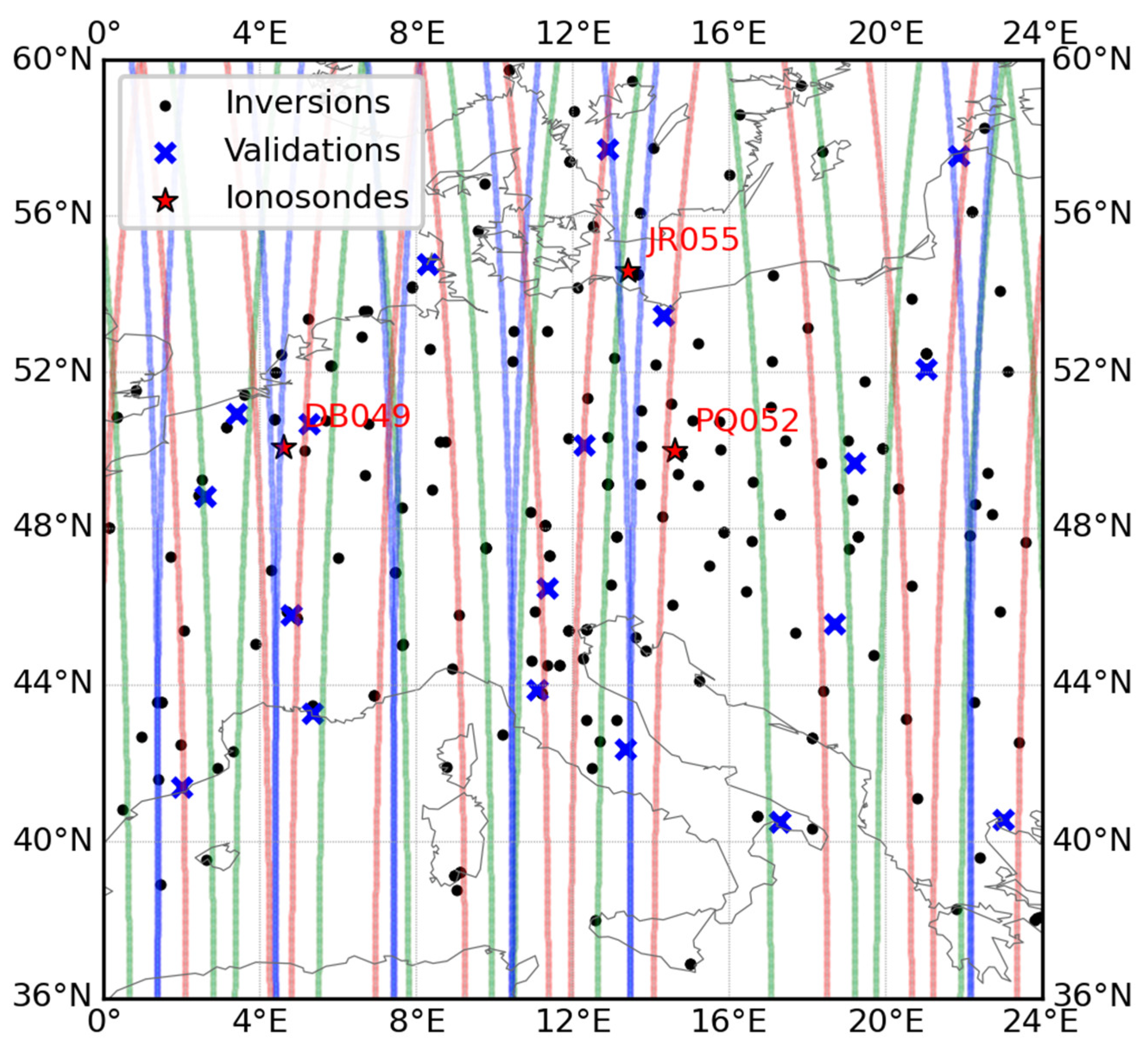
Six continuous days around the St. Patrick’s storm 2015 (from 15 to 20 March 2015) were selected to perform the tomographic inversion. The area of inversion covers the longitudes from 0° E to 24° E, the latitudes from 34° N to 60° N and the heights from 100 to 1200 km. In this area, 231 GNSS stations, 3 ionosonde stations and 53 continuous Swarm profiles are available (see Figure 2). Among all the GNSS stations, 21 (about 10%, see Table 1) were selected for independent validation purposes and hence removed from the inversion. The GNSS observation data were downloaded from the EUREF Permanent GNSS Network (http://www.epncb.oma.be/, accessed on 22 September 2022). The observations of peak density, peak height, ionosonde profile, Swarm observation and VTEC map were downloaded from the Lowell Global Ionosphere Radio Observatory (GIRO) Data Center (http://giro.uml.edu, accessed on 22 September 2022), the NOAA National Centers for Environmental Information (https://www.ngdc.noaa.gov/, accessed on 22 September 2022), Europe Space Agency (ESA) (https://earth.esa.int/, accessed on 22 September 2022) and the International GNSS Service (IGS) center(www.igs.org, accessed on 22 September 2022), respectively.

3.2. Validation Methods

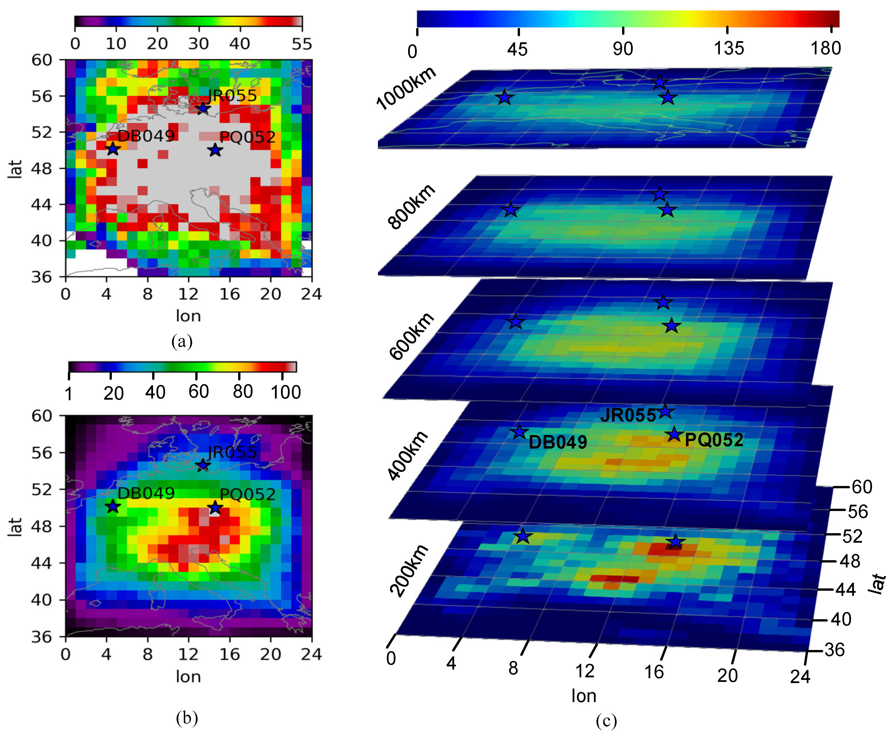
The inversion of STEC was achieved by a tool provided by the Ionospheric Research Group (www.ionolab.org, accessed on 22 November 2022) using a method described by Sezen et al. (2013). In this tool, the differential code bias (DCB) of the receivers was solved and removed jointly with the satellites’ DCBs, which were obtained from the Center for Orbit Determination in Europe (CODE). A horizontal resolution of 1 o and a vertical resolution of 20 km were adopted to divide the ionosphere into 24 × 24 × 55 voxels. Figure 3 shows the number of voxels that are traversed by the GNSS rays. As can be seen, not all voxels have traversing GNSS rays, but voxels in the center area are mostly covered by the rays.
The voxels in the model were filled with the initial electron density given by the background obtained from the same epoch based on the International Reference Ionosphere model 2016 (IRI2016) [45]. The two threshold values ( ζ and γ) were set to be 2σ and 25%, respectively, where σ stands for the standard deviation of the corrections. Other parameters in the tomographic inversion are presented in Table 2.
Parameters derived from the reconstructed image were compared with those obtained from ionosonde observations, Swarm satellite measurements, independent STEC observations and VTEC map. To evaluate the quality of the tomographic image, the root mean square error (RMS) between the constructed image and the various observations is computed as:
RMS =   ( x x 0 ) 2 n
where x stands for the derived parameter, x 0 refers to the truth-value and n represents the number of samples.
To make a further comparison, the MART algorithm was also implemented under the same condition as the RACR algorithm. The RMS ( RMS ) improvement for the RACR algorithm over the MART algorithm was computed as:
RMS = RMS ( R ) RMS ( M )
where RMS ( R ) refers to the RMS of the RACR algorithm, and RMS ( M ) represents the RMS of the MART algorithm. Note that a negative value of RMS indicates an improvement in the RACR algorithm over the MART algorithm.

4. Results

4.1. Validation with Ionosonde Vertical Profiles

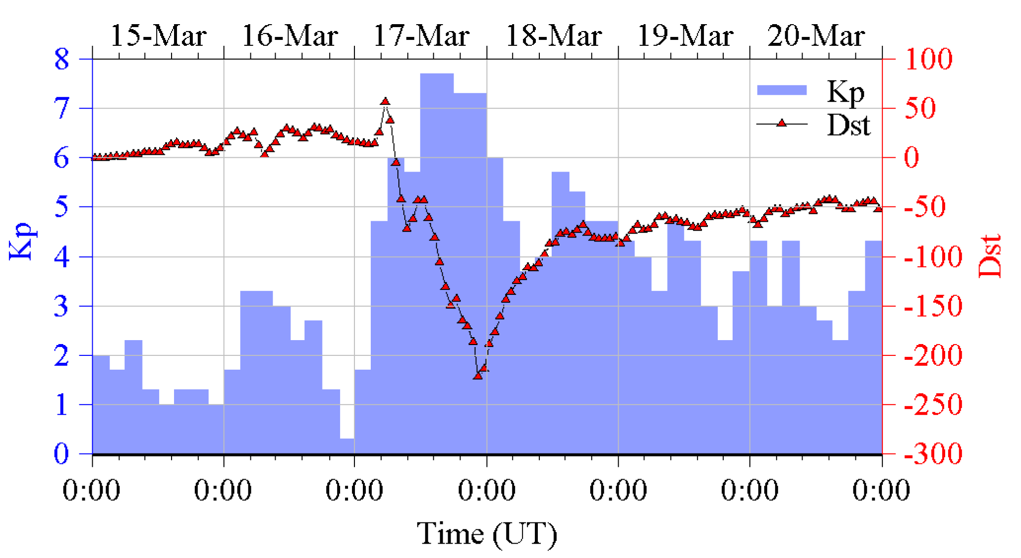
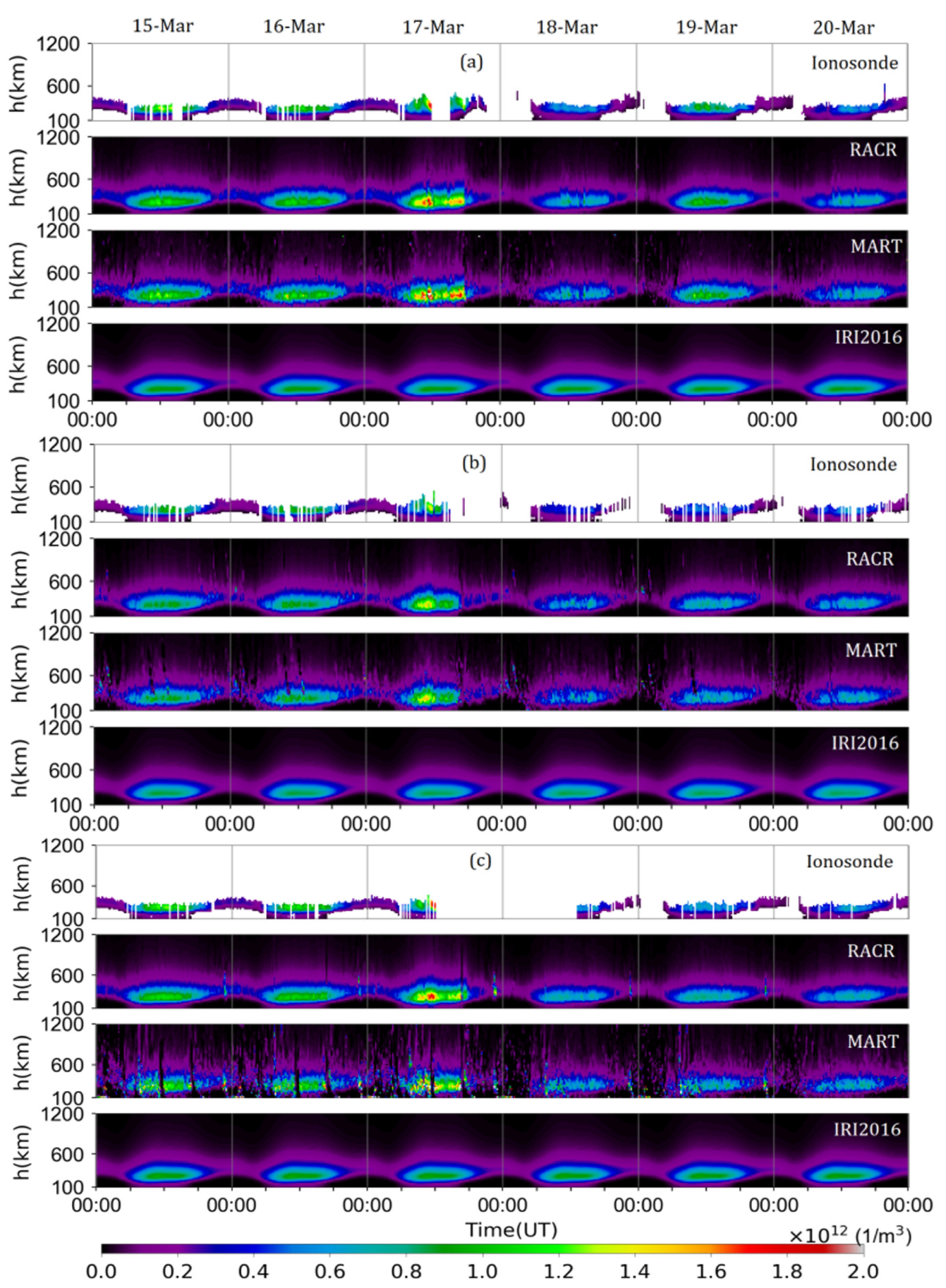
The 2015 St. Patrick’s Day storm is one of the strongest within the solar cycle 24 with a measured DST of −223 nT. Figure 4 depicts the temporal variations of the geomagnetic indices (Kp index and storm disturbance index) over the study period. As shown, the storm’s sudden commencement occurred at ~04:45 UT on 17 March 2015, with a decrease in Dst. The Kp index reached a maximum value of 7 during the period of Dst reaching minima. The main phase of the storm lasted for ~17 h and went into the recovery phase after 17 March 2015, and then ended at ~00:00 UT on 18 March 2015. Figure 5 shows the temporal variations of the vertical density from ionosonde observation, RACR image, MART image and IRI2016 model, respectively, at the three stations. Though some data are missing from the ionosonde observation, the storm impact is still observable from its temporal image. By contrast, the IRI model gives less information on the storm, as its images seem to be very similar over the whole period. Compared to the image of the IRI model, both MART images and RACR images are closer to the ionosonde image and are able to display the two phases of the storm. However, MART images are much noisier than RACR images, especially at station PQ052, where the main phase of the storm is difficult to observe in the MART image. Compared to the MART images, RACR images are smoother, and the two phases of the storm can be clearly observed.
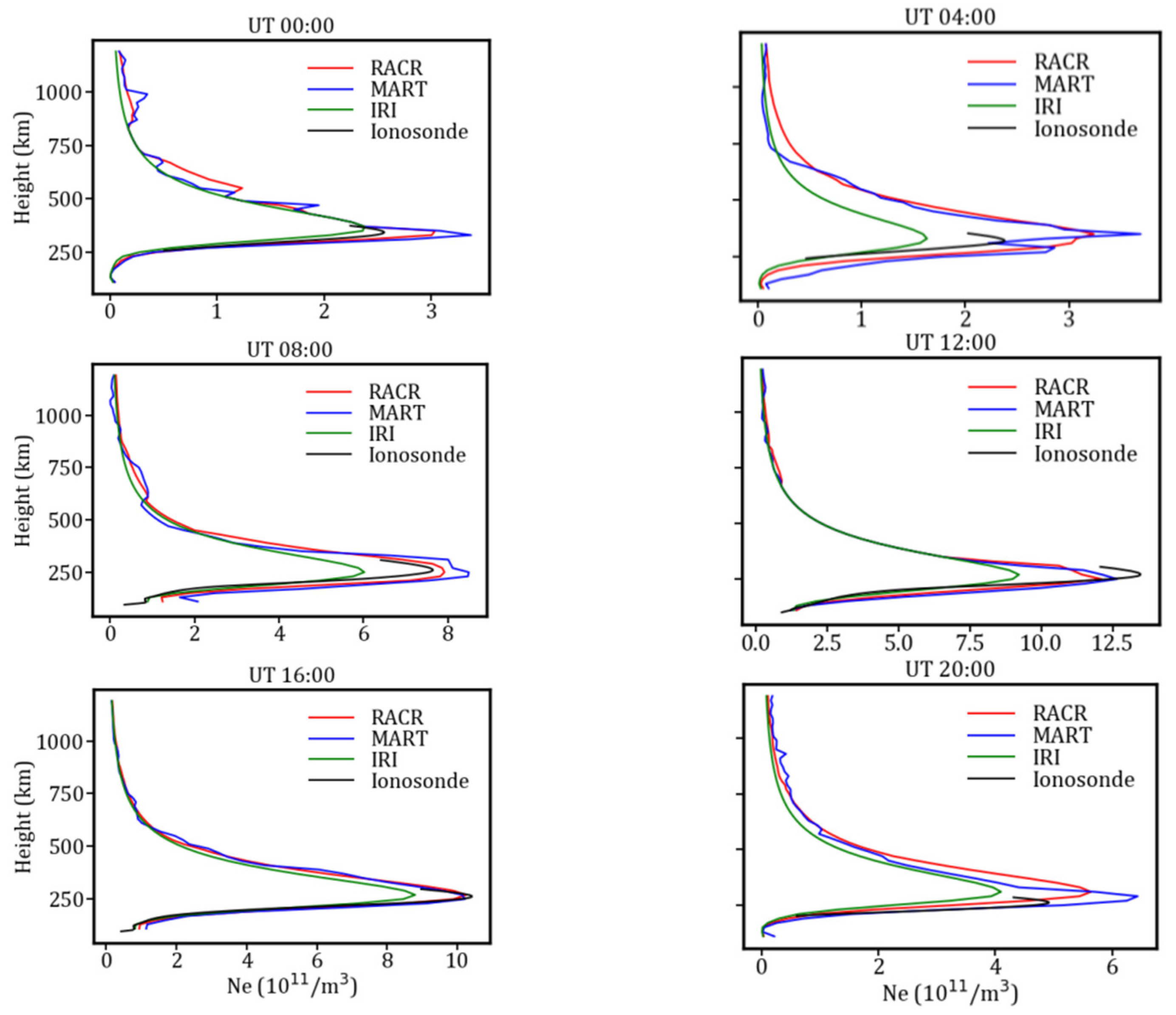
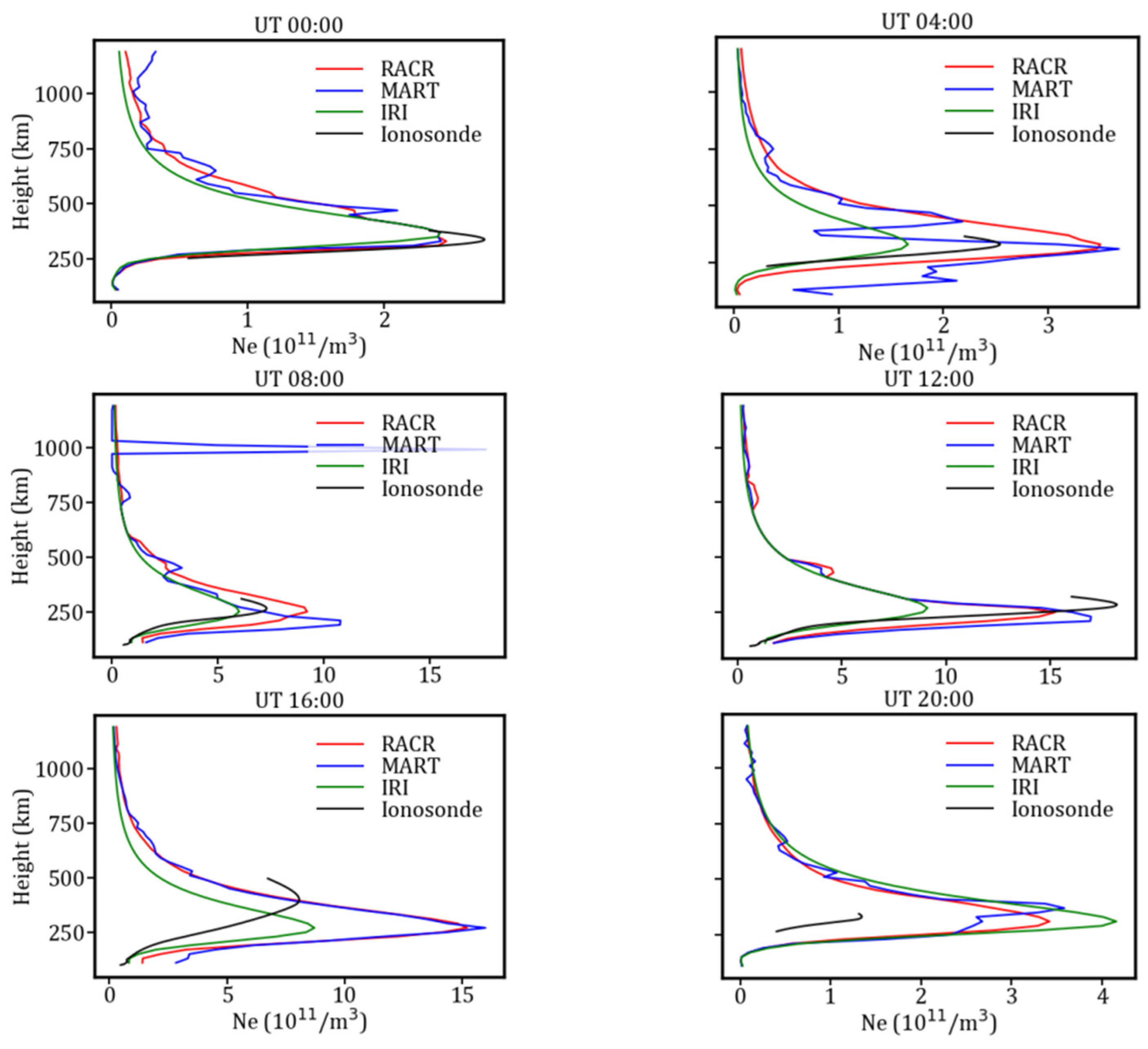
In the following analysis, we shall use profiles from station DB049 to illustrate the performances of the various methods due to consideration of the length of the paper. DB049 is selected because the MART algorithm has a better performance than PQ052 and has a similar performance to JR055. Figure 6 shows example vertical profiles at DB049 at four-hour intervals on March 15, a geomagnetically quiet day. As seen, the profiles of the RACR algorithm are closer to the ionosonde observation than those of the MART algorithm. In addition, the RACR algorithm-generated profiles are smoother and more realistic than those from the MART algorithm. Profiles from both RACR and MART are offset from the ionosonde observation at nighttime but exhibit a good agreement with the ionosonde observation in the daytime. The offset issue will be further discussed later in Section V. Figure 7 also shows vertical profiles at four-hour intervals at the same station on a disturbed day (17 March). Compared to the quiet day, while both algorithms deviate more from the ionosonde profiles on the disturbed day, the profiles of the RACR algorithm are closer to the ionosonde observations and are smoother than that of the MART algorithm.

4.2. Validation with Ionosonde NmF2 and hmF2

The peak density (NmF2) and the peak height (hmF2) of the F2 layer are two important parameters for determining the vertical structure of the ionosphere. Both are provided in ionosonde observations. To validate these two parameters, we derived them from the corresponding vertical profile based on the reconstructed image at each epoch and then compared them to the observations to get the errors, which were used to derive the RMS (both individual and overall) and then the RMS. It is not easy to determine the exact values of NmF2 and hmF2 from the image produced by the MART algorithm, as some of the vertical profiles have large fluctuations. To overcome this issue, we derived the two parameters by imposing a Chapman fitting on the corresponding profile that lies in the vertical range of 150 to 600 km altitude with a least square method. If the fitting operation fails, the maximum density and its corresponding height inside that vertical range are used as substitutes for the estimations.
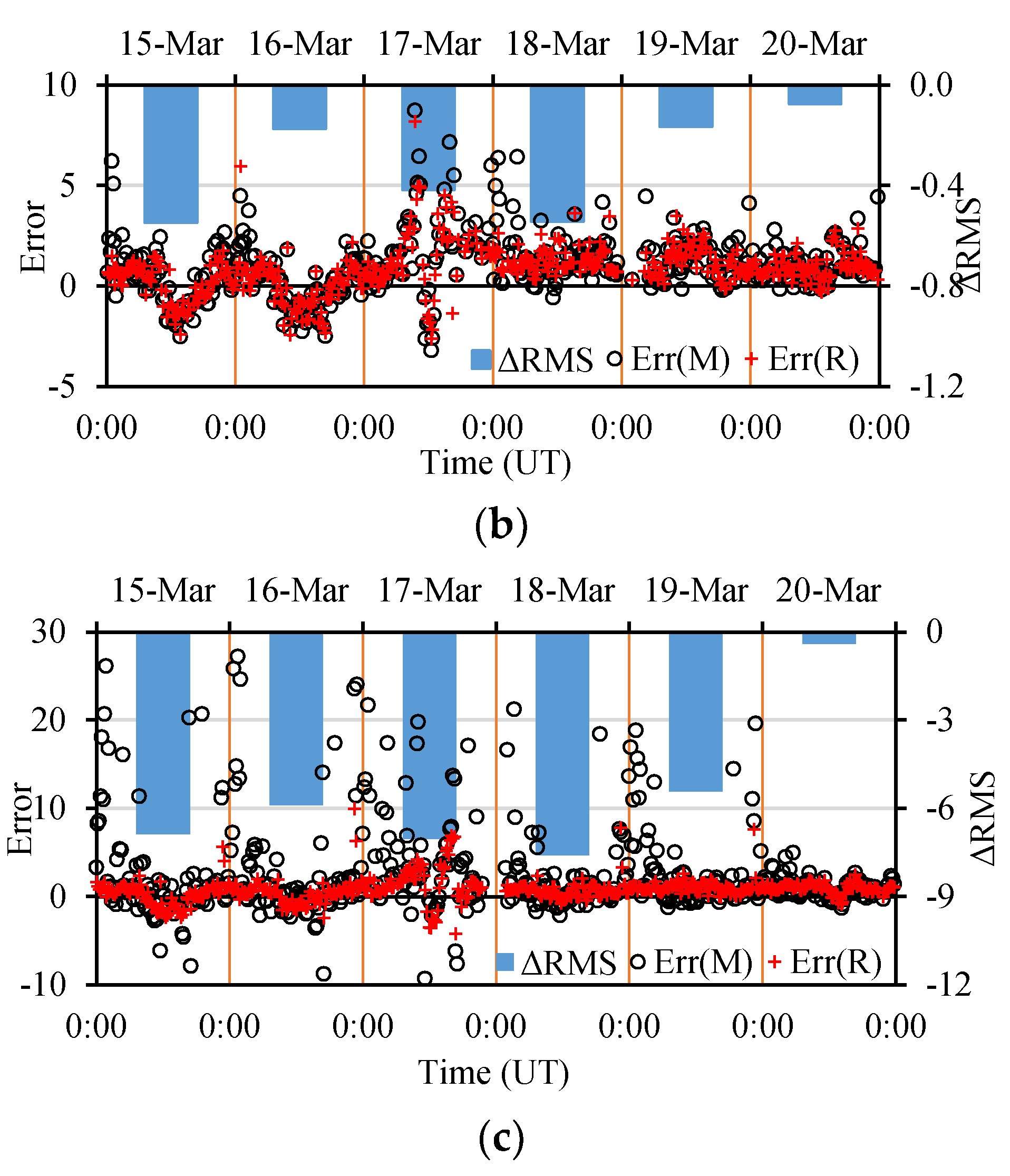
Figure 8 demonstrates the errors of both algorithms, as well as the RMS , for the NmF2 estimation at different sites. The errors of the RACR algorithm are smaller than those of the MART algorithm, and the RMSs are always negative, which suggests that the RACR algorithm performs better than the MART algorithm. The superiority is most obvious at station PQ052, which happens to be at the center of the research area (see Figure 3b), where more associated GNSS rays are available for the voxels above the station compared to the other two stations. Having more associated GNSS rays means that more data can be used in the corrections of the voxels. Statistically, more data (i.e., STEC observations) can produce a more accurate estimation if an averaging operation is employed. Compared to the MART algorithm, the RACR algorithm makes full use of these data, removes the abnormal values, and then makes a weighted averaging of these corrections, and hence produces a more accurate result. Another reason for the better performance at PQ052 is due to the poor performance of the MART algorithm itself. As can be seen from Figure 8, the errors of the MART algorithm at PQ052 seem to be much larger than that at the other two stations. This may be due to errors in the STEC data at this particular site. More data means more errors are involved. In the MART algorithm, the errors of correction caused by rays, especially the abnormal rays, can be accumulated through the process of iterations. By contrast, the abnormal corrections and rays are removed, and hence the propagation of error is restrained in the RACR algorithm.
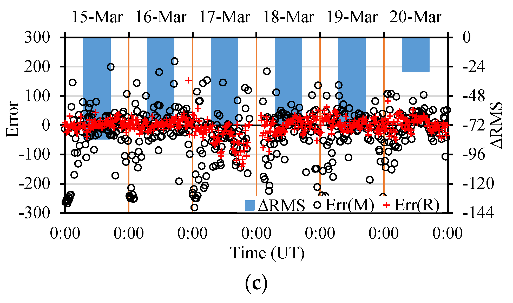
Figure 9 depicts the errors of both algorithms, as well as the RMS, for hmF2 estimation at the three sites. Like the results shown in NmF2 estimation, the errors of hmF2 estimation for the RACR algorithm are smaller than that for the MART algorithm. All the RMS are negative, which also suggests that the RACR algorithm works better than the MART algorithm. Again, the improvement of RACR over MART is most prominent at the PQ052 station for the hmF2 estimation for the same reasons discussed above.
Table 3 lists the overall RMS of the estimated NmF2 and hmF2 at the three stations for both algorithms and the IRI2016 model. As for the estimated NmF2, the RACR algorithm performs the best, followed by the MART algorithm and then the IRI2016 model. The MART algorithm performance at the PQ052 station is the worst. The average improvement of the RACR algorithm over the MART algorithm on NmF2 is 36.01% for all three stations. As for the estimated hmF2, IRI2016 and the RACR algorithm are very close, while the MART algorithm is significantly off. The average improvement of the RACR algorithm over the MART algorithm on hmF2 is 36.56% for all three stations.

4.3. Validation with Swarm Satellites

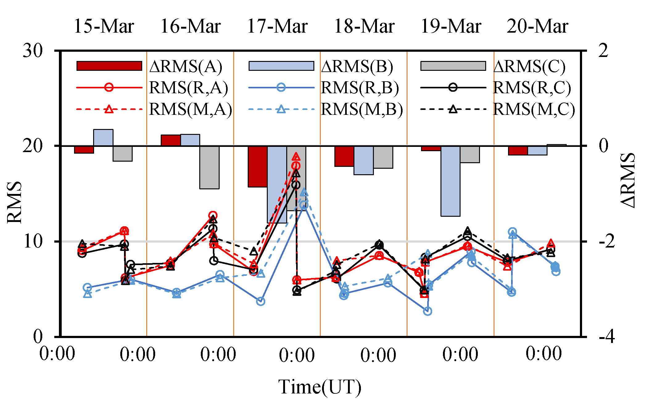
The ground-based ionosonde can measure only the bottom side of the ionosphere up to the height of the F2-layer peak. However, Swarm satellites, which were launched by the European Space Agency (ESA) at the end of 2013, provide measurements of electron density for the topside ionosphere. The mission consists of three satellites (Alpha (A), Bravo (B) and Charlie (C)), among which A and C are placed at an orbit of about 450 km and B at about 510 km. All of them measure the ionosphere at a rate of 2 Hz, which produces a much denser sampling than the tomographic inversion. To make the result comparable, we interpolated the electron density of the tomographic image according to the sampling points of the Swarm measurements and calculated the difference between the reconstructed image and the Swarm measurements. An RMS value is computed for each continuous profile, and an overall RMS is evaluated for each day. The overall RMS is then used to produce the RMS each day.
Figure 10 depicts the individual RMS and its corresponding RMS . The results of MART and RACR are very close. Their accuracies are about 1 × 10¹¹/m3 on quiet days and about 2 × 10¹¹/m3 on disturbed days. The RACR algorithm exhibits a slight improvement over the MART algorithm, as indicated by the dominantly negative RMS values. The overall RMS during the entire period, which is presented in Table 4, also confirms this conclusion. The RACR algorithm achieves the best performance for all three satellites. The MART algorithm performs better than the IRI2016 model on Swarms A and B but slightly worse on Swarm C. The average improvement in the RACR algorithm over the MART algorithm is 6.18% for all three satellites.

4.4. Validation with Independent STEC

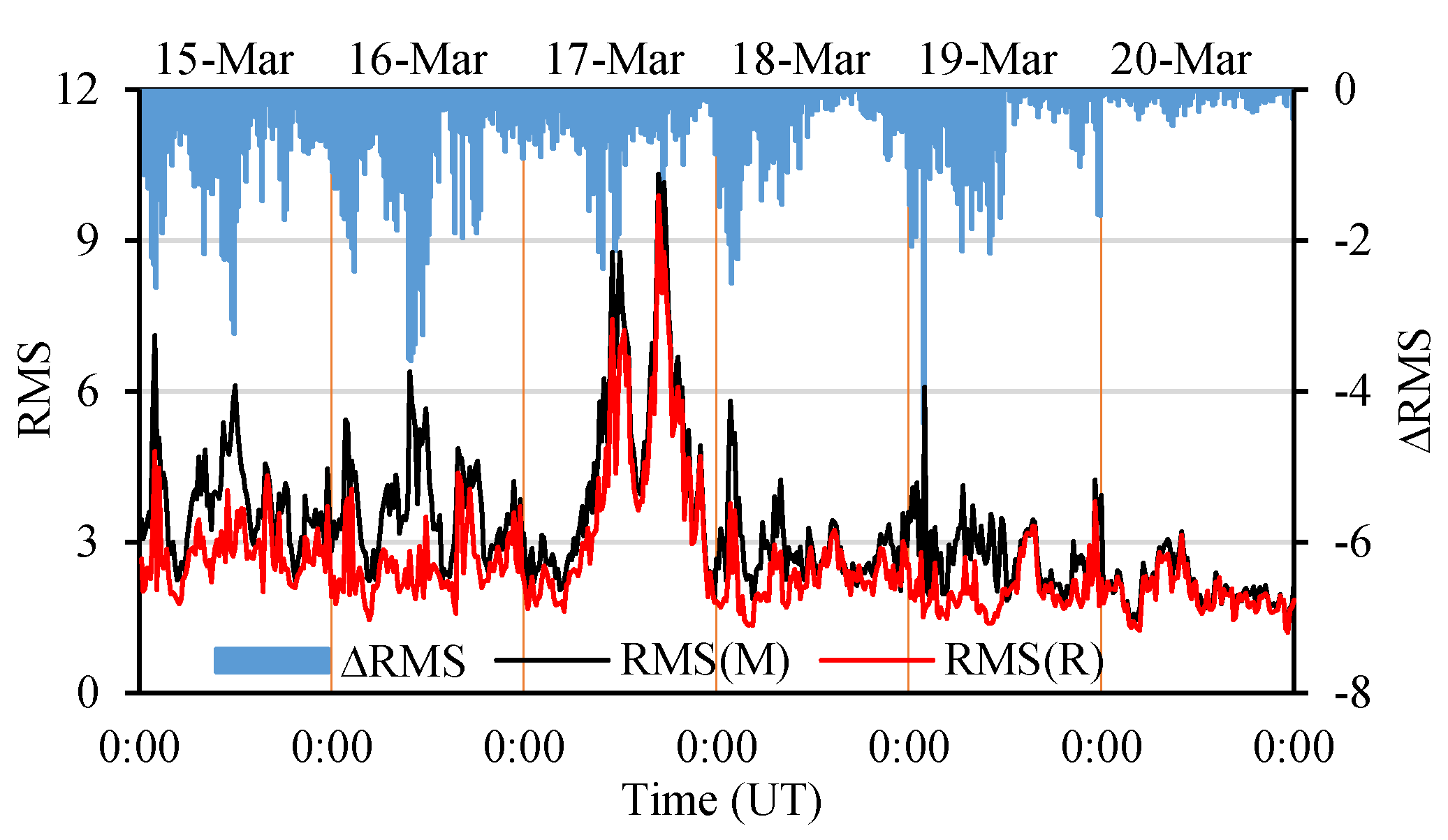
By taking independent GNSS observations as the ground-truth references, the STEC error along each GNSS ray was computed for both algorithms. The errors in the same epoch were then used to compute the RMS for 15-min intervals. The differences in the RMS, i.e., RMS between the two algorithms, were calculated. Figure 11 shows the RMS for the MART and RACR and their RMSs. Nearly all the RACR RMS values are lower than those of the MART. However, the improvement of RMS for the RACR algorithm varies over time. The improvement on 20 March is very limited. However, for the remaining days, including two disturbed days, the improvement reaches about 1 TECU on average. Table 5 presents the overall RMS over the entire period for the two algorithms and the IRI2016 model. It is clear that the RACR algorithm outperforms the MART algorithm and the IRI2016 model, and the MART algorithm performs better than the IRI2016 model. The improvement in the overall RMS for the RACR algorithm over the MART algorithm is 22.10%.

4.5. Validations with VTEC Map

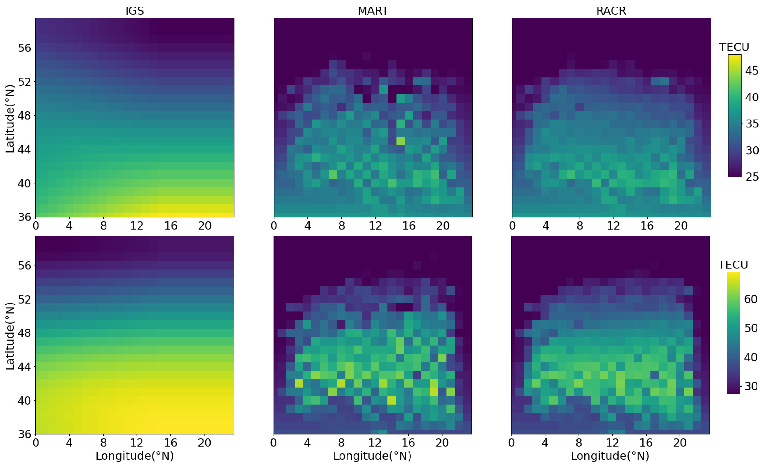
The VTEC products provided by IGS were also used to validate the RACR and MART algorithms. Figure 12 shows the VTEC maps produced by IGS, MART and RACR on a quiet geomagnetic day and a geomagnetically disturbed day, respectively. The two maps produced by RACR and MART are similar to those provided by IGS in those pixels with many passing rays (see Figure 3) but differ a lot in those pixels with very few passing rays, where they are the same as the background. Despite this, the maps produced by RACR are less noisy than those by MART. The reason is that abnormal rays, which are responsible for the noises, are rejected in RACR. Table 6 gives the overall RMS of the VTEC by taking IGS as the truth. As seen, RACR outperforms MART and IRI-2016. The improvement of RACR over MART on the VTEC map is 6.03% during the whole period.

5. Discussions

5.1. Night Time Vertical Profiles Offset

In Figure 6 and Figure 7, both RACR and MART algorithms show an apparent offset from the ionosonde observation at nighttime but exhibit a good agreement with the ionosonde observation in the daytime. This is likely due to the contribution of the plasmasphere to the observed STEC, which is ignored in this study. The plasmasphere’s contribution to the overall STEC is more significant in the nighttime than in the daytime. To confirm it, we performed an additional test by removing the topside STEC derived by the IRI-Plus model [46] from the observed STEC. Figure 13 shows that the estimated profile is visibly improved after using the corrected STEC value in the nighttime. However, the correction appears to have degraded the daytime results, as shown in the right panel of Figure 13. The correction can, on the one hand, remove the bias caused by the topside ionosphere, but, on the other hand, may also introduce an additional error brought by the empirical model. Therefore, the topside STEC should be removed during inversion at nighttime as it may significantly improve the image quality. However, it is not advisable to remove it as it contributes very little in the daytime, and the additional errors introduced by the empirical model may have an important impact on the reconstructed image.

5.2. Determinations of Thresholds

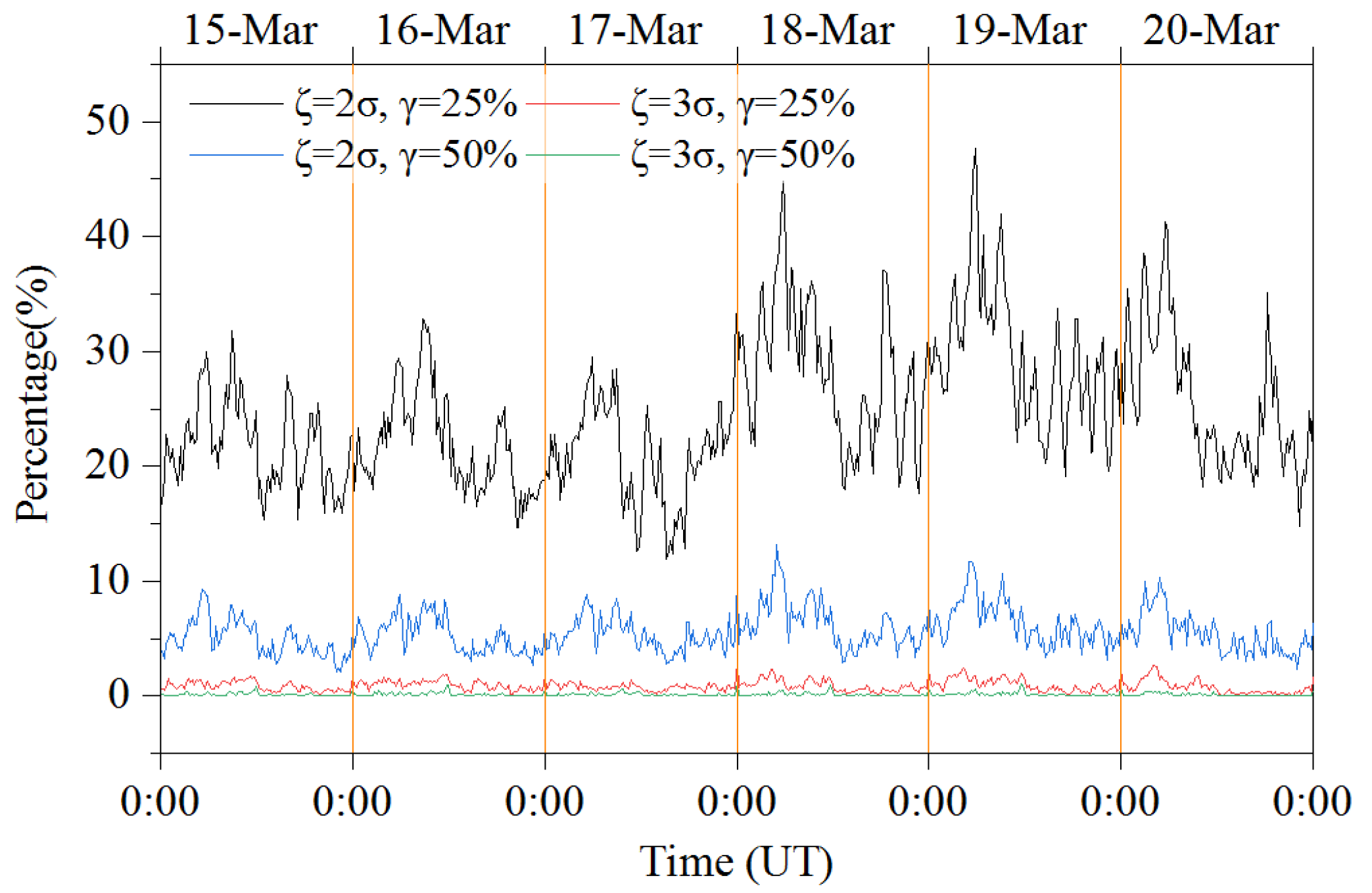
In the RACR algorithm, an abnormal correction is determined if the value lies outside a normal range defined by ζ . However, such a decision could be a wrong one. The impact of a wrong decision could be very limited for a voxel with many associated rays, as there are many other corrections still available that can keep the correction process under check. A smaller ζ tends to confine the corrections of a voxel to a limited range, which would lead to a smoother image, and vice versa. If a ray is rejected by a voxel but it does not contain an abnormal value on STEC, the ray should not be removed from successive iterations. However, it is difficult for a single voxel to distinguish a normal STEC from an abnormal one. In the RACR algorithm, a ray with a rejected ratio that exceeds γ is considered to be an abnormal ray. Therefore, a larger γ would decrease the probability of making a wrong decision regarding the abnormal ray (false alarms), but at the same time would increase the risk of a missed detection of an abnormal ray, and vice versa. Figure 14 compares several vertical profiles with different ζ and γ for a quiet day (left panel) and a disturbed day (right panel). As seen, profiles with smaller ζ and γ tend to be smoother. It should be noted that smoothness does not indicate accuracy. In the case of Figure 14a,b, the smoother curves are indeed more accurate. However, that is not the case for Figure 14c,d, where normal rays were rejected due to a wrong decision. However, smoother profiles are associated with better performances, especially for the cases where rays contain many errors.
Figure 15 presents the percentage of rays that are rejected by the RACR algorithm in each epoch. Smaller ζ and γ tend to reject more rays. As more abnormal rays are rejected, the images would be smoother. This is also confirmed by Figure 14, where profiles with smaller ζ and γ (e.g., ζ = 2 σ , γ = 20 % versus ζ = 3 σ , γ = 50 % ) and more rejected rays (e.g., ζ = 2 σ , γ = 50 % versus ζ = 3 σ , γ = 25 % ) tend to be smoother.
To examine whether the rejected rays are indeed abnormal ones, Figure 16 shows the vertical profiles produced by the MART algorithm employing only rays where outliers had been removed based on the RACR algorithm and all available rays. As shown, the results from using rays without outliers are closer to the ionosonde observations and are smoother than the results from the ones obtained using all available rays. Therefore, we can infer that the rejected rays are mostly abnormal rays, and the rejection of abnormal rays improves the quality of the tomographic image.

6. Conclusions

STEC data obtained from GNSS observations often contain errors that may lead to abnormal corrections for those voxels in which the corresponding rays traverse for the tomographic inversion. Multiple iterations of correction will result in an accumulation of errors in the imaging results. To prevent the abnormal corrections from contaminating an image, a correction threshold is introduced to define a normal range of correction for each voxel in this paper. A correction that is outside of this range is considered an abnormal correction and is then removed from the averaging correction for that voxel. The abnormal correction information is then extended to calculate the rejected ratio of a ray, which is used to decide whether it is an abnormal ray based on a given threshold of the rejected ratio. Abnormal rays are finally removed from subsequent iterations to make the reconstructed image smoother and more accurate.
The proposed algorithm is validated with ionosonde stations, Swarm satellite measurements, independent STEC observations and the VTEC map are also compared with the MART algorithm during a period of six continuous days when a geomagnetic storm occurred. The proposed algorithm RACR is able to capture the main and recovery phases of the storm very clearly in the inverted image. The results show that the removal of abnormal rays improves image quality. RACR outperforms the MART algorithm under both quiet and stormy geomagnetic conditions. The RACR’s average improvement over the MART algorithm is 36.01%, 36.56%, 6.18%, 22.10% and 6.03% in the validation tests of NmF2, hmF2, topside electron density, STEC and VTEC, respectively. The quality of the produced image using RACR is controlled by two thresholds, i.e., ζ and γ . The results show that a smaller threshold value tends to make the image smoother.
The RACR algorithm provides not only a way to produce a better tomographic image but also a possible solution to detect an abnormal ray. Despite this, several things still need to be performed to make the algorithm more robust. For example, how to decide on an optimal value for the two thresholds remains challenging. Our future work will focus on the further validation of the rejected rays by comparing them with other observation data, the optimization of the threshold values and after the incorporation of other strategies, such as additional constraints and regularization, into our tomographic model to make the image even better.

Author Contributions

J.Z. and C.J. implemented the method, J.Y. contributed the main ideas and wrote the manuscript, Y.D., Y.Z. and Y.H. carried out the tests and analyzed the data and L.W. reviewed and edited the manuscript. All authors have read and agreed to the published version of the manuscript.

Funding

This research was jointly funded by the National Natural Science Foundation of China grant number 41771416, the China Postdoctoral Science Foundation grant number 2017M611949, and the National Key Research and Development Program of China grant number 2018YFC1503505.

Institutional Review Board Statement

Not applicable.

Informed Consent Statement

Not applicable.

Data Availability Statement

Data sharing not applicable.

Acknowledgments

We thanked Jade Morton and Zhe Yang for providing some constructive suggestions to this paper. We also thanked the anonymous reviewers whose suggestions greatly improved the quality of this paper.

Conflicts of Interest

The authors declare that they have no conflicts of interest to disclose.

References

  1. Bust, G.S.; Mitchell, C.N. History, current state, and future directions of ionospheric imaging. Rev. Geophys. 2008, 46, RG1003. [Google Scholar] [CrossRef]
  2. Prol, F.S.; Themens, D.R.; Hernndez-Pajares, M.; Paulo, O.C.; Muella, M.T.A.H. Linear Vary-Chap Topside Electron Density Model with Topside Sounder and Radio-Occultation Data. Surv. Geophys. 2019, 40, 277–293. [Google Scholar] [CrossRef]
  3. Austen, J.R.; Franke, S.J.; Liu, C.H.; Yeh, K.C. Application of computerized tomography techniques to ionospheric research. In Proceedings of the International Beacon Satellite Symposium on Radio Beacon Contribution to the Study of Ionization and Dynamics of the Ionosphere and to Corrections to Geodesy and Technical Workshop, Oulu, Finland, 9–14 June 1986; pp. 25–32. [Google Scholar]
  4. Garcia, R.; Crespon, F. Radio tomography of the ionosphere: Analysis of an underdetermined, ill-posed inverse problem, and regional application. Radio Sci. 2008, 43, 1–13. [Google Scholar] [CrossRef] [Green Version]
  5. Jin, S.; Li, D. 3-D ionospheric tomography from dense GNSS observations based on an improved two-step iterative algorithm. Adv. Space Res. 2018, 62, 809–820. [Google Scholar] [CrossRef]
  6. Yu, J.Q.; Wang, W.Y.; Holden, L.; Liu, Z.P.; Wu, L.X.; Zhang, S.L.; Zhang, K.F. Enhancing the Quality of Tomographic Image by Means of Image Reconstruction Based on Hybrid Grids. Adv. Space Res. 2020, 66, 591–603. [Google Scholar] [CrossRef]
  7. Wen, D.; Yuan, Y.; Ou, J.; Zhang, K.; Liu, K. A hybrid reconstruction algorithm for 3-D ionospheric tomography. IEEE Trans. Geosci. Remote Sens. 2008, 46, 1733–1739. [Google Scholar] [CrossRef] [Green Version]
  8. Yao, Y.; Chen, P.; Zhang, S.; Chen, J. A new ionospheric tomography model combining pixel-based and function-based models. Adv. Space Res. 2013, 52, 614–621. [Google Scholar] [CrossRef]
  9. Lu, W.; Ma, G.; Wan, Q.; Li, J.H.; Wang, X.L.; Fu, W.Z.; Maruyama, T. Virtual reference station-based computerized ionospheric tomography. GPS Solut. 2021, 25, 8. [Google Scholar] [CrossRef]
  10. Zhou, C.; Fremouw, E.J.; Sahr, J.D. Optimal truncation criterion for application of singular value decomposition to ionospheric tomography. Radio Sci. 1999, 34, 155–166. [Google Scholar] [CrossRef]
  11. Bhuyan, K.; Singh, S.B.; Bhuyan, P.K. Tomographic reconstruction of the ionosphere using generalized singular value decomposition. Curr. Sci. 2002, 83, 1117–1120. [Google Scholar] [CrossRef]
  12. Raymund, T.D.; Austen, J.R.; Franke, S.J.; Liu, C.H.; Klobuchar, J.A.; Stalker, J. Application of computerized tomography to the investigation of ionospheric structures. Radio Sci. 1990, 25, 771–789. [Google Scholar] [CrossRef]
  13. Prol, F.S.; Camargo, P.d.O.; Pajares, M.H.; Muella, M.T.A.H. A New Method for Ionospheric Tomography and Its Assessment by Ionosonde Electron Density, GPS TEC, and Single-Frequency PPP. IEEE Trans. Geosci. Remote Sens. 2019, 57, 2571–2582. [Google Scholar] [CrossRef]
  14. Kamp, M.J.L. Medium-scale 4-D ionospheric tomography using a dense GPS network. Ann. Geophys. 2013, 31, 75–89. [Google Scholar] [CrossRef] [Green Version]
  15. Seemala, G.; Yamamoto, M.; Saito, A.; Chen, C. Three-dimensional GPS ionospheric tomography over Japan using constrained least squares. J. Geophys. Res.-Space 2014, 119, 3044–3052. [Google Scholar] [CrossRef] [Green Version]
  16. Chen, C.H.; Saito, A.; Lin, C.H.; Yamamoto, M.; Suzuki, S.; Seemala, G.K. Medium-scale traveling ionospheric disturbances by three-dimensional ionospheric GPS tomography. Earth Planets Space 2016, 68, 1–9. [Google Scholar] [CrossRef] [Green Version]
  17. Tang, J.; Yao, Y.; Zhang, L.; Kong, J. Tomographic reconstruction of ionospheric electron density during the storm of 5-6 August 2011 using multi-source data. Sci. Rep. 2015, 5, 13042. [Google Scholar] [CrossRef] [Green Version]
  18. Prol, F.S.; Manuel, H.P.; Muella, T.A.H.M.; Camargo, P.D.O. Tomographic imaging of ionospheric plasma bubbles based on GNSS and radio occultation measurements. Remote Sens. 2018, 10, 1529. [Google Scholar] [CrossRef] [Green Version]
  19. Wang, S.; Huang, S.; Lu, S.; Yan, B. 3-D ionospheric tomography using model function in the modified L-Curve method. IEEE Trans. Geosci. Remote Sens. 2019, 57, 3135–3147. [Google Scholar] [CrossRef]
  20. Li, H.; Yuan, Y.; Li, Z.; Huo, X.; Yan, W. Ionospheric Electron Concentration Imaging Using Combined of LEO Satellites Data with Ground-based GPS Observations over China. IEEE Trans. Geosci. Remote Sens. 2012, 50, 1728–1735. [Google Scholar] [CrossRef]
  21. Ssessanga, N.; Yamamoto, M.; Saito, S.; Saito, A.; Nishioka, M. Complementing regional ground GNSS-STEC computerized ionospheric tomography (CIT) with ionosonde data assimilation. GPS Solut. 2021, 25, 93. [Google Scholar] [CrossRef]
  22. Zheng, D.Y.; Yao, Y.B.; Nie, W.F.; Liao, M.; Liang, J.; Ao, M. Ordered Subsets-Constrained ART Algorithm for Ionospheric Tomography by Combining VTEC Data. IEEE Trans. Geosci. Remote Sens. 2021, 59, 7051–7061. [Google Scholar] [CrossRef]
  23. Cushley, A.C.; Noel, J.M. Ionospheric sounding and tomography using Automatic Identification System (AIS) and other signals of opportunity. Radio Sci. 2020, 55, e2019RS006872. [Google Scholar] [CrossRef]
  24. Yu, J.Q.; Yang, Z.; Breitsch, B.; Wu, L.X. Fast Determination of Geometric Matrix in Ionosphere Tomographic Inversion with Unevenly Spaced Curvilinear Voxels. GPS Solut. 2022, 26, 1–14. [Google Scholar] [CrossRef]
  25. Lu, W.; Ma, G.; Wan, Q. A Review of Voxel-Based Computerized Ionospheric Tomography with GNSS Ground Receivers. Remote Sens. 2021, 13, 3432. [Google Scholar] [CrossRef]
  26. Kondo, T.; Hobiger, T.; Koyama, Y. Constrained simultaneous algebraic reconstruction technique (C-SART)—A new and simple algorithm applied to ionospheric tomography. Earth Planets Space 2008, 60, 727–735. [Google Scholar] [CrossRef] [Green Version]
  27. Sui, Y.; Fu, H.; Wang, D.; Xu, F.; Feng, S.; Cheng, J.; Jin, Y. Sparse Reconstruction of 3-D Regional Ionospheric Tomography Using Data From a Network of GNSS Reference Stations. IEEE Trans. Geosci. Remote Sens. 2022, 60, 4102615. [Google Scholar] [CrossRef]
  28. Zhu, H.Y.; Yu, J.Q.; Dai, Y.C.; Zhu, Y.Y.; Huang, Y.Q. Ionosphere Tomographic Model Based on Neural Network with Balance Cost and Dynamic Correction Using Multi-Constraints. Atmosphere 2022, 13, 426. [Google Scholar] [CrossRef]
  29. He, L.M.; Heki, K. Three-dimensional tomography of ionospheric anomalies immediately before the 2015 Illapel earthquake, Central Chile. J. Geophys. Res. Space 2018, 123, 4015–4025. [Google Scholar] [CrossRef] [Green Version]
  30. Razin, M.R.G.; Voosoghi, B. Regional Ionosphere Modeling Using Spherical Cap Harmonics and Empirical Orthogonal Functions over Iran. Acta Geod. Geophys. 2017, 52, 19–33. [Google Scholar] [CrossRef] [Green Version]
  31. Farzaneh, S.; Forootan, E. Reconstructing Regional Ionospheric Electron Density: A Combined Spherical Slepian Function and Empirical Orthogonal Function Approach. Surv. Geophys. 2018, 39, 289–309. [Google Scholar] [CrossRef]
  32. Minkwitz, D.; Boogaart, K.G.; Gerzen, T.; Hoque, M.M. Tomography of the Ionospheric Electron Density with Geostatistical Inversion. Ann. Geophys. 2015, 33, 1071–1079. [Google Scholar] [CrossRef]
  33. Tang, J.; Gao, X. Adaptive Regularization Method for 3-D GNSS Ionospheric Tomography Based on the U-Curve. IEEE Trans. Geosci. Remote Sens. 2021, 59, 4547–4560. [Google Scholar] [CrossRef]
  34. Ciraolo, L.; Azpilicueta, F.; Brunini, C.; Meza, A.; Radicella, S.M. Calibration errors on experimental slant total electron content (TEC) determined with GPS. J. Geod. 2007, 81, 111–120. [Google Scholar] [CrossRef]
  35. Nie, W.; Xu, T.; Rovira-Garcia, A.; Zornoza, J.M.J.; Subirana, J.S.; Gonzalez-Casado, G.; Chen, W.; Xu, G.C. Revisit the calibration errors on experimental slant total electron content (TEC) determined with GPS. GPS Solut. 2018, 22, 1–14. [Google Scholar] [CrossRef] [Green Version]
  36. Ssessanga, N.; Kim, Y.H.; Habarulema, J.B.; Kwak, Y.S. On Imaging South African Regional Ionosphere Using 4D-var Technique. Space Weather 2019, 17, 1584–1604. [Google Scholar] [CrossRef] [Green Version]
  37. Andersen, A.H.; Kak, A.C. Simultaneous Algebraic Reconstruction Technique (SART): A superior implementation of the ART algorithm. Ultrason. Imaging 1984, 6, 81–94. [Google Scholar] [CrossRef] [PubMed]
  38. Gerzen, T.; Minkwitz, D. Simultaneous multiplicative column-normalized method (SMART) for 3-D ionosphere tomography in comparison to other algebraic methods. Ann. Geophys. 2016, 34, 97–115. [Google Scholar] [CrossRef] [Green Version]
  39. Yu, J.Q.; Wang, Y.; Zhu, Y.Y.; Huang, Y.Q.; Wu, L.X. Iterative tomography method for ionosphere inversion via parameters smoothing. Chin. J. Geophys. 2022. [Google Scholar] [CrossRef]
  40. Prol, F.D.; Camargo, P. Ionospheric tomography using GNSS: Multiplicative algebraic reconstruction technique applied to the area of Brazil. GPS Solut. 2016, 20, 807–814. [Google Scholar] [CrossRef] [Green Version]
  41. Yang, Z.; Song, S.; Jiao, W.; Chen, G.M.; Xue, J.C.; Zhou, W.L.; Zhu, W.Y. Ionospheric tomography based on GNSS observations of the CMONOC: Performance in the topside ionosphere. GPS Solut. 2017, 21, 363–375. [Google Scholar] [CrossRef]
  42. Li, W.; Wang, G.; Mi, J.; Zhang, S. Calibration errors in determining slant Total Electron Content (TEC) from multi-GNSS data. Adv. Space Res. 2019, 63, 1670–1680. [Google Scholar] [CrossRef]
  43. Brunini, C.; Azpilicueta, F.J. Accuracy assessment of the GPS-based slant total electron content. J. Geod. 2009, 83, 773–785. [Google Scholar] [CrossRef]
  44. Strode, P.; Groves, P. GNSS multipath detection using three-frequency signal-to-noise measurements. GPS Solut. 2016, 20, 399–412. [Google Scholar] [CrossRef] [Green Version]
  45. Gulyaeva, T.L. International standard model of the earth’s inosphere and plasmasphere. Astraonomy Astrophys. 2003, 22, 639–643. [Google Scholar] [CrossRef]
  46. Bilitza, D.; Altadill, D.; Truhlik, V.; Shubin, V.; Galkin, I.; Reinisch, B.; Huang, X. International Reference Ionosphere 2016: From ionospheric climate to real-time weather predictions. Space Weather 2017, 15, 418–429. [Google Scholar] [CrossRef]
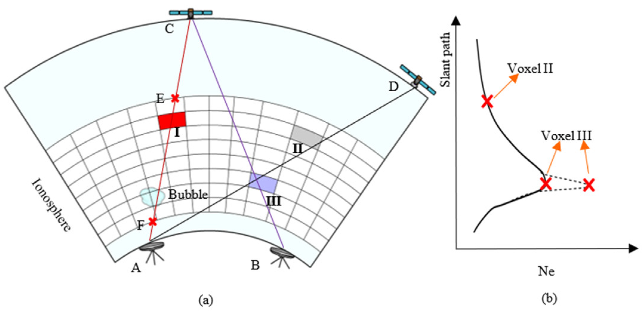
Figure 1. Causes of abnormal correction in a voxel. (a) Sketch of voxels, a bubble and rays in a tomographic model. Usually, the whole STEC of the ray AC is adopted in tomographic inversion due to the difficulty in removing the contribution of the plasmasphere (i.e., the part of CE). However, only part of the EF should be responsible for the tomographic inversion. (b) Sketch of abnormal correction in a particular ray. Suppose that the solid profile shown on the right is the current state of ray AD shown on the left, and there is an abnormal correction on voxel III brought by ray BC. The abnormal correction will certainly lead to the model STEC along ray AD being unusually larger or smaller, which, in turn, may result in an abnormal correction for other associated voxels, e.g., voxel II.
Atmosphere 13 01954 g001
Figure 2. Distribution of GNSS stations, ionosonde stations and the trajectories of Swarm satellites over the study period. Black dots and blue crosses are the GNSS stations for inversions and validations, respectively. Red stars are ionosonde stations. Blue, red and green lines are the trajectories of Swarm satellites.
Atmosphere 13 01954 g002
Figure 3. Voxels covered by GNSS rays. (a) The number of voxels that are traversed by GNSS rays in each vertical column (i.e., pixel) at 00:00 universal time (UT) on 15 March 2015 with white color indicating that none of the voxels were crossed in that column. (b) The average number of associated rays for the voxels in a vertical column during the whole study period. The value of each pixel is computed by the sum of the associated ray number in each column divided by the number of voxels in each column (i.e., 55 here), and then averaged over the whole period. (c) The average number of associated rays at different heights for the voxels during the whole study period.
Atmosphere 13 01954 g003
Figure 4. Kp and Dst indices with UT hour on 15–20 March 2015.
Atmosphere 13 01954 g004
Figure 5. Temporal variations in vertical density at ionosonde station (a) DB049, (b) JR055 and (c) PQ052 over the study period. The four rows (from top to bottom) in each subplot correspond to the results of ionosonde, RACR algorithm, MART algorithm and IRI2016 model, respectively. Pixels with no data are filled with white color.
Atmosphere 13 01954 g005
Figure 6. Comparisons of electron density profile at station DB049 at four-hour intervals on 15 March 2015 starting at UT 00:00.
Atmosphere 13 01954 g006
Figure 7. Comparisons of electron density profile at station DB049 at four-hour intervals on 17 March 2015.
Atmosphere 13 01954 g007
Figure 8. The error (unit: 1011/m3) and the RMS (unit: 1011/m3) of the derived NmF2 at ionosonde stations (a) DB049, (b) JR055 and (c) PQ052 with the ionosonde observations as the ground-truth. “M” and “R” in the bracket refer to the MART algorithm and RACR algorithm, respectively. Each point of the data for the error corresponds to an error in each epoch, and each column of the data for the RMS corresponds to the statistic of the whole day. Notice that the scales of the error and the RMS for (c) are several times that of the other two.
Atmosphere 13 01954 g008aAtmosphere 13 01954 g008b
Figure 9. The error (unit: km) and the RMS (unit: km) of the derived hmF2 at ionosonde stations (a) DB049, (b) JR055 and (c) PQ052. “M” and “R” in the brackets refer to the MART algorithm and RACR algorithm, respectively. Each point of the data for the error corresponds to an error at each epoch, and each column of the data for the RMS corresponds to the statistic of the whole day. Notice that the scale of RMS for (c) is four times that of the other two.
Atmosphere 13 01954 g009aAtmosphere 13 01954 g009b
Figure 10. The individual RMS (unit: 1010/m3) and its corresponding RMS (unit: 1010/m3) of the reconstructed electron density with the Swarm measurements as the truth-value. “M”, “R”, “A”, “B” and “C” in the brackets refer to the MART algorithm, RACR algorithm, Swarm A, Swarm B and Swarm C, respectively. Each point of the data for the RMS corresponds to the statistic of a continuous profile, and each column of the data for the RMS corresponds to the statistic of the whole day.
Atmosphere 13 01954 g010
Figure 11. The individual RMS (unit: TECU) and its corresponding RMS (unit: TECU) of the derived STEC with the GNSS observation as the ground-truth. “M” and “R” in the brackets refer to the MART and RACR algorithms, respectively. Each point of data corresponds to an epoch.
Atmosphere 13 01954 g011
Figure 12. VTEC maps produced by IGS (left panels), MART (middle panels) and RACR (right panels) at UT 12:00 March 15, 2015 (top panels) and at UT 12:00 March 117 (bottom panels).
Atmosphere 13 01954 g012
Figure 13. Comparisons of electron density profile at station DB049 on 15 March 2015 for the result after STEC correction against those without STEC correction. The curve with a suffix of “_c” corresponds to the result with STEC correction, and vice versa. The epochs for the left and right panels are UT 01:00 and UT 12:00, respectively.
Atmosphere 13 01954 g013
Figure 14. Comparisons of vertical profiles with different ζ and γ . (a) March 16, 2015 at station PQ052, (b) 17 March 2015 at station PQ052, (c) 15 March 2015 at station PQ052, (d) 18 March at station JR055. σ in the figures stands for the standard derivation. Notice that the solid red and solid blue are almost overlapped in (a,b), solid red, solid blue and red dash are overlapped in (c) and solid blue, blue dash and red dash are almost overlapped in (d).
Atmosphere 13 01954 g014
Figure 15. Percentage of rays that were rejected by the RACR algorithm at each epoch. σ in the figures stands for the standard derivation.
Atmosphere 13 01954 g015
Figure 16. Comparisons of vertical profiles produced by the MART algorithm employing only rays where outliers had been removed based on the RACR algorithm and all available rays at ζ = 2 σ, γ = 25 % . Both figures were generated by the MART algorithm on 18 March 2015. The left panel is for DB049, and the right panel is for PQ052.
Atmosphere 13 01954 g016
Table 1. The 4-Letter code of GNSS stations selected for independent STEC validation.
AQUIFATAJOZ2POUSZYWI
AUT1GELLMARSPRAT
BCLNHOE2MDORSPT0
BZRGHOERMLVLTARS
DENTIRBEOSJEWARE
Table 2. Several parameters used in the tomographic inversions.
λ Times of IterationTemporal ResolutionElevation Cut-Off
0.0550015 min25o
Table 3. The overall RMS of the estimated NmF2 (unit: 1011/m3) and hmF2 (km) for both algorithms and the IRI2016 model over the study period.
AlgorithmIonosondeRMS (NmF2)RMS (hmF2)
RACRDB0491.5936.22
JR0551.4637.89
PQ0521.6228.92
MARTDB0491.8043.32
JR0551.7849.79
PQ0527.5094.44
IRI2016DB0491.9636.04
JR0551.9032.42
PQ0521.9427.76
Table 4. The overall RMS of the reconstructed electron density (unit: 1010/m3) by the RACR algorithm, MART algorithm and IRI2016 model over the study period.
AlgorithmSwarm ASwarm BSwarm C
RACR9.396.799.18
MART9.697.479.80
IRI201610.117.799.76
Table 5. The overall RMS (unit: TECU) of the derived VTEC by the RACR algorithm, MART algorithm and IRI2016 model over the whole study period.
RACRMARTIRI2016
RMS2.753.539.26
Table 6. The overall RMS (unit: TECU) of the derived VTEC by the RACR algorithm, MART algorithm and IRI2016 model over the whole study period.
RACRMARTIRI-2016
RMS4.995.317.51
Publisher’s Note: MDPI stays neutral with regard to jurisdictional claims in published maps and institutional affiliations.