Spatiotemporal Patterns of Air Pollution in an Industrialised City—A Case Study of Ust-Kamenogorsk, Kazakhstan

Abstract

Air quality issues still affect the quality of life for people in industrialised cities around the world. The investigations should include the identification of the sources of the pollution and its distribution in space and time. This work is the first attempt to perform identification of the sources of pollution in Ust-Kamenogorsk city in Kazakhstan. Analysis of retrospective data (including ten variables (TSP, SO₂, CO, NO₂, phenol, HF, HCl, H₂SO₄, formaldehyde, H₂S) from five monitoring stations for the period 2017–2021) using multivariate statistical methods and hierarchical cluster analysis has been performed to assess spatiotemporal patterns of air quality of the city. The results indicate that the contamination patterns can be grouped into two categories: cold and warm seasons. The study revealed the dangerous concentrations of NO₂ and SO₂ exceeded the limits by 2–3 and 1.5–2 times, independently of the seasonality. Averaged concentrations of TSP slightly exceeded the established limits for the most industrialised part of the city. Concentrations of HF and formaldehyde significantly rose during the cold seasons compared to the warm seasons. Other chemical parameters significantly depend on the seasonality and locations of the sampling points. The major reason for air pollution is twofold—the use of a burnt-coal throughout the year for electricity and heat generation (especially during the cold seasons) and the high density of the heavy metallurgy industry in the city. The principal component analysis confirms a high loading of industrial sources of air pollution on both spatial and seasonal dimensions.

1. Introduction

In 2022 humanity still faces air pollution issues, while it is much known about efficient ways to handle them. Statistics revealed the significant pollution in big cities, even in countries where the possibility for permanent monitoring with the wide web of monitoring stations has been established [1]. At the same time, the situation can be much worse in developing countries, especially in industrialised cities, as the cities have not been connected to the common database and the ability to assess environmental and social consequences has been hidden. Studies say that despite direct hazards to health and the economy, the influence and the interests of big manufacturing and energy companies sometimes can prevail over the mentioned issues and exert pressure on regulatory aspects [2]. These factors make the air pollution issues still actual around the world. For instance, a study by Yuan et al. [3] claims that cities with pollution-intensive industries are responsible for urban air pollution (called “super emitters” as they dominate as large point sources of pollution [4]). According to another study by Gu et al. [5], the industrial sector has been recognised as the largest contributor to air pollution among all sectoral emitters in China. Industrial activities led to accounting for 36% of the total impact on health, including premature mortalities, as well as 41% of crop production loss over the whole country. The authors estimated that the scenario that mainly reduces industrial emissions would provide the largest air quality benefits among various scenarios. A sound work by Burnett et al. says that 8.9 million deaths, even as early as in the year 2015, could have been caused by poor air quality worldwide [6]. An SDG’s Indicator 3.9.1 states that the mortality rate attributed to household and ambient air pollution should be substantially reduced by 2030 to ensure healthy lives and promote well-being for all.

Kazakhstan is a developing country which sets a collection of the mentioned problems in the context of air pollution. Obsolete and non-conventional equipment in the main emitters [7], especially in the metallurgy sector [8], legislative loopholes [9], denying or slowing implementation of clean technologies [10], and drawbacks in the monitoring systems [11] have brought Kazakhstan to the list of countries with severe air conditions [12]. While Kazakhstan formally aims to achieve SDGs, including a healthy environment and good health for all, there is a lot to do, including air quality problems [13].

One of the problematic cities in the country, Ust-Kamenogorsk, is located in a major mining and smelting area and has been rated among the worst cities regarding the problems of ecology according to World Bank [14]. Extreme pollution events from accidental emissions are not rare in the city [15]. Descriptive studies of poor air quality in the city have said that the city has been rated the most SO₂-polluted city in Kazakhstan and among the five most-polluted NO₂ and O₃ cities in Kazakhstan from 2011 to 2017 [12]. A study about the impact of COVID-19 lockdown on air quality in the city has revealed that the level of CO has decreased by 21–23% with the increase in the TSP level by 13–21%, and had no significant effect on SO₂ and NO₂ concentrations in the city [16]. Elevated levels of trace elements, particularly Ba, Mn, Pb, V, and Zn, in the blood of city residents of Ust-Kamenogorsk have been found [17], which could indicate a severe impact on the industrial activities of the city. The known studies are limited by their descriptive origin, while there is a demand for deep investigations of the relationships between a high level of air pollution, weak environmental regulation, pyrometallurgical processes and dependence on coal-burnt energy.

Air quality plans apply the following measures for emission reduction: policy implications, control for technical feasibility, calculating resulting costs, source apportionment techniques, and assessment of the impact on the environment and human health. All these measures are based on the assurance of establishing and monitoring the exceedances of the air quality standards [18]. Also, a comprehensive emission inventory coupled with air quality monitoring is the first step to developing an emission control strategy for selected pollutants [19]. These tools do not work on their own, and pollution treatment programs have to come forefront [20]. Stricter environmental regulation leads to a reduction in polluting industrial activities on the way to the green economy and using environmentally-friendly advanced technologies [21]. As a result, embedding advanced control technologies within sustainable development policy scenarios would result in significant cost savings [22]. However, it also can lead to the closure of emitters or their relocation, which negatively impacts economic growth [23].

According to an opinion from [24], preliminary investigations play a core role in the identification of the sources of pollution to drive “the wheel of progress: Sources ⇒ Effects ⇒ Regulation ⇒ Control”. There are known different ways to investigate potential sources apportionment: emission inventories [25], inverse modelling [26], artificial neural networks [27], receptor modelling methods [28], air quality models [25], a combination of the different approaches and models [29], application of positive matrix factorisation [30], and even chemical analysis of biomonitoring species [31]. However, all of the listed methods demand a very detailed dataset with a number of monitored parameters. This limitation is a serious obstacle in the conditions of many developing countries, including Kazakhstan, where the system of permanent monitoring with extended parameters, such as PMs, has still been established [32].

Under these conditions, one of the efficient ways to investigate sources apportionment with the following understanding of the needed steps for air quality management can be multivariate statistical techniques, particularly Principal Component Analysis (PCA) and Cluster Analysis. In addition, using analysis of scores and loadings in PCA can give a representation of potential chemical reactions in ambient air [33]. The approach to applying PCA for the assessment of patterns in air quality has already been applied several times. For instance, Dominick et al. [34] aimed to investigate possible sources of air pollutants and spatial patterns in Malaysia using the same techniques as the authors plan to do with grouping particulate contaminants in principal components. Application of the PCA to find the correlation between gaseous pollutant concentrations, meteorological factors and potential sources of pollution has identified the contribution of combustion- and non-combustion-related emitters in Greece [35] or in India [36]. The tool has been used for the same purpose also by Azid et al. in the context of the prediction of air pollution [37]. PCA has supported the assessment and identification of the sources of air pollution in India, where complex industrial activities exist [38]. Revealing information about the sources and mechanisms of air pollution in Madrid and visualising their spatial distribution using PCA and the geostatistical method has been carried out by Núñez-Alonso et al. [39]. Particular attention has been paid to the investigation of the presence of metals only in particulate matters coupled with multivariate statistical techniques in an Iranian industrial city [40]. For example, a combination of the analysis of the chemical composition of fine particulate matters with the focus on metals presence with Absolute Principal Component Analysis allowed attributing the identified pollutants to their sources in the USA [41].

The aim of this study is to analyse key factors impacting air quality in Ust-Kamenogorsk using the available dataset for the period 2017–2021 by multivariate statistical techniques on spatial and temporal scales. This approach enables us to investigate potential sources of apportionment using the large but limited dataset of the observations in the city for the first time.

2. Materials and Methods

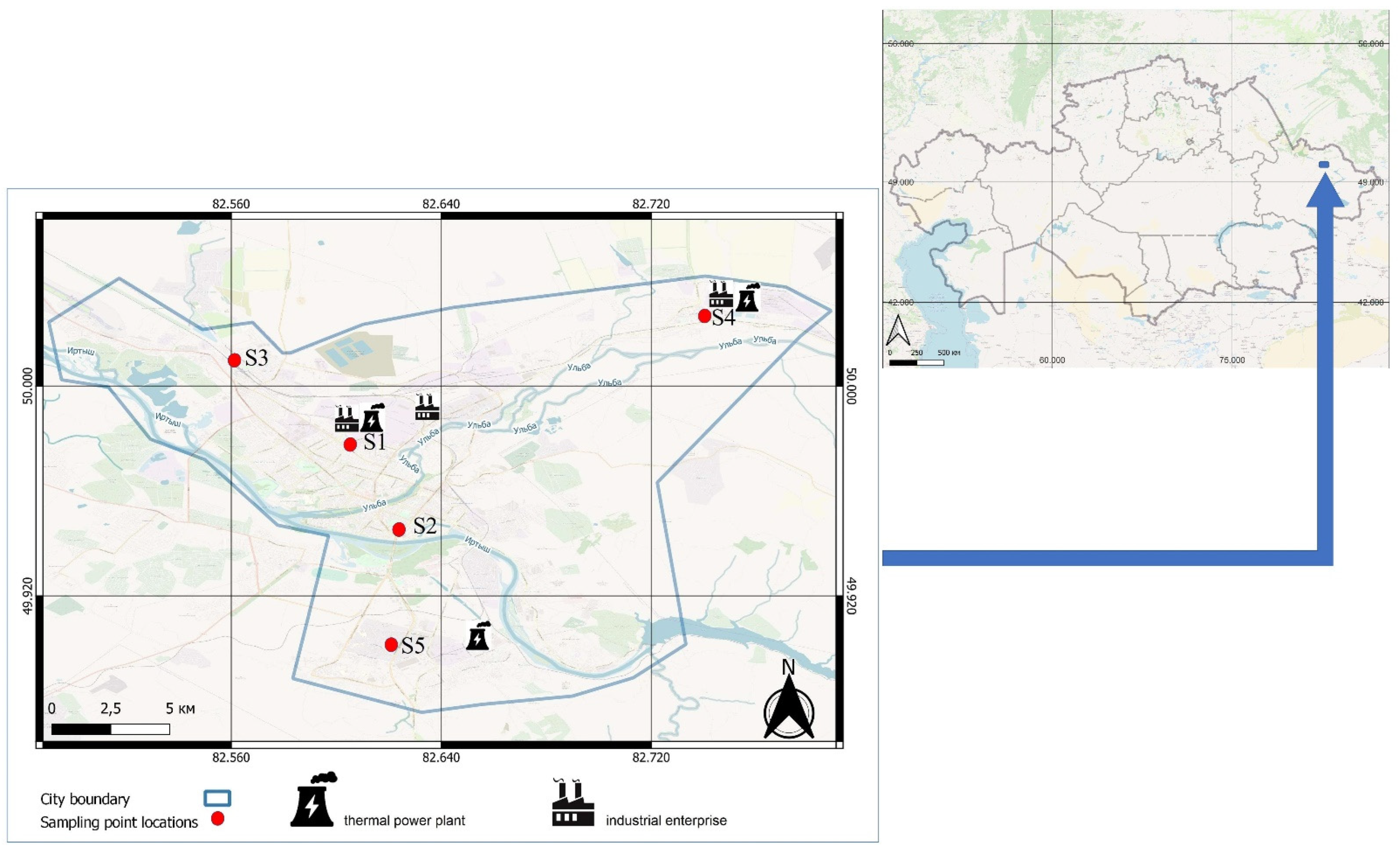
2.1. Study Area

Ust-Kamenogorsk (or Oskemen) is located in northeastern Kazakhstan in the foothills of the Altay and at a confluence of the Irtysh and the Ulba rivers. The climate of the Ust-Kamenogorsk region is temperate continental. The city is divided into two parts by the Irtysh River. The city is surrounded by Shanovsky and Kalbinsky mountain ranges on the southeastern site [42].

A number of the largest Kazakhstani metallurgy plants for the production of non-ferrous metals are located in the city: the metallurgical complex of Kazzinc LLP, the Ulba metallurgical plant, and the Ust-Kamenogorsk titanium and magnesium plant. Coupled with the Ust-Kamenogorsk and the Sogrinskaya thermal power plants, the industrial activities put significant pressure on the air conditions of the city. The locations of the main industries are presented in Figure 1. The main characteristics of the industries of the city are presented in

Table 1. Characteristics of the industrial enterprises of Ust-Kamenogorsk.

Enterprise	Production	The Volume of the Production	Permitted Emissions, t/y
The Ust-Kamenogorsk metallurgy complex of Kazzinc LLP	Lead Zinc Copper Technical sulfuric acid	144 Kt/y 190 Kt/y 70 Kt/y 1000 Kt/y	TSP—129; NO2—245; SO2—16,856; H2SO4—51; CO—8356; HF—12; HCl—57; H2S—0.5
The Ulba metallurgical plant	Tantalum Uranus Beryllium	No open data	TSP—7.4; NO2—5; SO2—0.1; H2SO4—4.4; CO—0.5; HF—2.3; HCl—0.7
The Ust-Kamenogorsk thermal power plant	Heat energy Electricity Burnt coal	859.9 Gcal/h 372.5 MW/y 1.5 Mt/y	TSP—3035; NO2—4470; SO2—9277; CO—185; HF—0.006; H2S—0.001
The Ust-Kamenogorsk titanium and magnesium plant	Titanium tetrachloride Sponge titanium Raw magnesium Anhydrous carnallite	49 Kt/y 12 Kt/y 13 Kt/y 9.6 Kt/y	TSP—24; NO2—15; SO2—30; H2SO4—0.1; CO—314; HF—0.14; HCl—28
The Sogrinskaya thermal power plant	Heat energy Electricity Burnt coal	168 Gcal/h 75 MW/y 0.35 Mt/y	TSP—454; NO2—975; SO2—1974; CO—8
The left-bank thermal power plant	Heat energy Burnt coal	168 Gcal/h 0.083 Mt/y	TSP—693; NO2—342; SO2—446; CO—95

.

The city can be conditionally divided into three zones: two big industrial areas (the northern and the northeastern industrial zones), and downtown, located on the left bank of the Irtysh River, with its own thermal power plant. The northern industrial zone includes the locations of the Ust-Kamenogorsk metallurgical complex of Kazzinc LLP, the Ulba metallurgical plant, and the Ust-Kamenogorsk thermal power plant. The northeastern industrial zone includes the Ust-Kamenogorsk titanium-magnesium plant and Sogrinskaya thermal power station. Accordingly, five monitoring stations (noted as S1–S5 in Figure 1) are located for sampling and analysis of the air quality:

-

Station 1—is located in the northern industrial zone;

-

Station 2—is located in the administrative centre of the city;

-

Station 3—is located in the north-western part of the city, adjacent to the northern industrial zone;

-

Station 4—is located in the northeastern industrial zone;

-

Station 5—is located downtown.

2.2. Multivariate Statistical Techniques

Correlation analysis, principal components analysis (factor analysis), and hierarchical cluster analysis were applied to identify the multivariate relationships between different variables and samples in the study area. The dataset was normalised for the elimination of the effect from differences in units (Equation (1)).

$$Z_{ij}=\frac{\left(x_{ij}-m_i\right)}{\mathrm{SD}},$$

(1)

where Z_ij are normalised values from x_ij, i is the represented variables, j is the sample number, m_i is the mean value, and SD is the standard deviation of the sample.

The relation between each pair of variables was measured by Pearson’s correlation coefficient to determine the associations among different variables. Correlation coefficients greater than 0.5 were considered significant. PCA recognises the most significant parameters from a big dataset of inter-correlated parameters and creates independent variables (Equation (2)).

$$z_{ij}=a_{i1}{x}_{1j}+a_{i2}{x}_{2j}+\dots +a_{im}{x}_{mj},$$

(2)

where z is the component score, a is the component loading, x is the measured value of a variable, i is the component number, j is the sample number, and m is the total number of variables. Factor analysis (FA) is a similar approach to PCA. However, PC is presented as a linear combination of parameters. FA follows PCA and takes into account unobservable, hypothetical, latent variables. They are included in the equation with the special residual term (Equation (3)).

$$z_{ij}=a_{f1}{f}_{1j}+a_{f2}{f}_{2j}+\dots +a_{fm}{x}_{mj}+e_{fi},$$

(3)

where z is the measured variable, a is the factor loading, f is the factor score, e is the residual term according to errors or another source of variation, i is the sample number, and m is the total number of factors.

Cluster analysis was used to assemble similar groups of the monitoring dates due to similarities between their variables. Hierarchical agglomerative CA provided Ward’s linkage distance, reported as D_link/D_max, which represents the quotient between the linkage distances for each case divided by the maximal linkage distance. The produced dendrogram enables analysing similarities easily. Ward’s linkage and the Euclidean distance as similarity measurements are commonly used for cluster analysis for the assessment of air quality [43].

All mathematical and statistical computations were performed using Microsoft Office Excel 2016 and IBM SPSS Statistics 26 software.

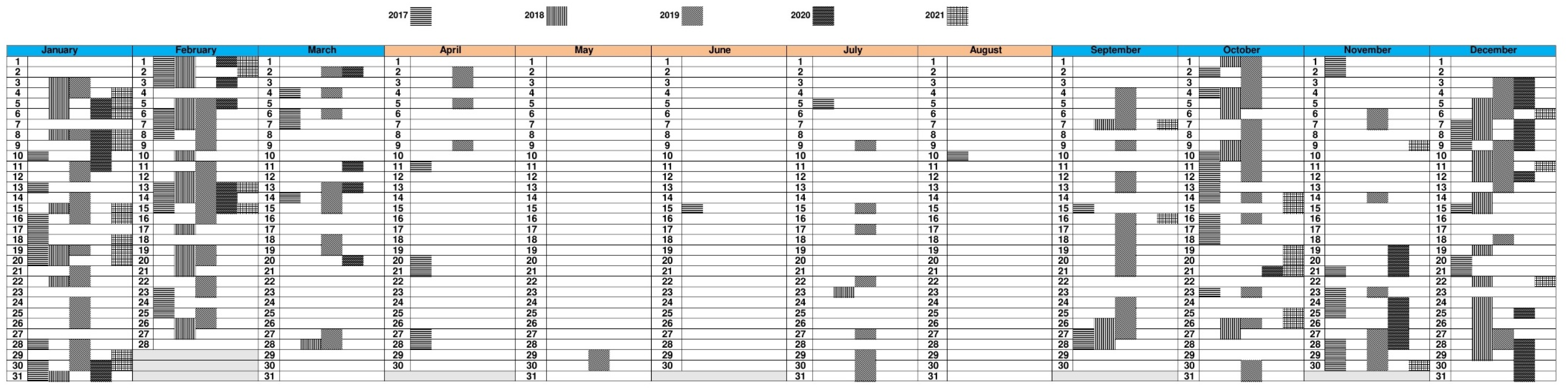
2.3. Data Management and Methodological Framework

The National Hydrometeorological Service of Kazakhstan “Kazhydromet” has provided a raw dataset for this study. Equipment, lab, staff, and methodology of analysis are certified and follow national and international standards for QC/QA. The dataset contains the results of manual measurements of 17 contaminants. Most of these measurements have been carried out four times per day at five stations (Figure 1). To obtain the most detailed picture, ten contaminants have been chosen for spatiotemporal and statistical assessment: total suspended particles (TSP); SO₂; CO; NO₂; phenol; HF; HCl; H₂SO₄; formaldehyde; and H₂S for the period 2017–2021. The reason for the selection of these contaminants and this period is the fullest available dataset, as they have been measured on a regular daily basis, except for weekends and vacations. It is important to note that TSP is not a commonly used parameter worldwide, while information about common worldwide contaminants particulate matter (PM) has not been provided due to its absence. Information about temperature, wind speed, wind direction, and humidity has been obtained from the archive of the web resource www.rp5.kz (accessed on 15 November 2022) [44] to identify possible interconnections with meteorological conditions of the region.

The first step of the analysis was to identify potentially similar periods in a matter of contamination. This step includes hierarchical clustering analysis, which was performed for each studied year separately with the following evaluation and identification of the grouped periods. Dates against daily averaged values of contaminants have been used as parameters for this analysis. The daily averaged values of the contaminants were also used for the second step: performing descriptive statistical analysis to evaluate air pollution in general for the selected temporal clusters. The number of daily averaged observations was 859 and 602 for the cold and warm seasons for all the monitored contaminants. The spatiotemporal assessment was the third step of this study and included time series and spatial analysis using geoinformation systems. Monthly averaged values were used to identify and evaluate trends in air pollution through the studied period, while mean values for the whole period were used for the spatial assessment. Interpolation using the inverse distance method was used to describe the distribution of the contamination within the city [45]. The fourth step of this study was to perform PCA based on the correlation matrix. The correlation matrix was built using daily averaged values of the studied contaminants coupled with the meteorological parameters, while the PCA was completed using chemical parameters only on a daily averaged measurements basis.

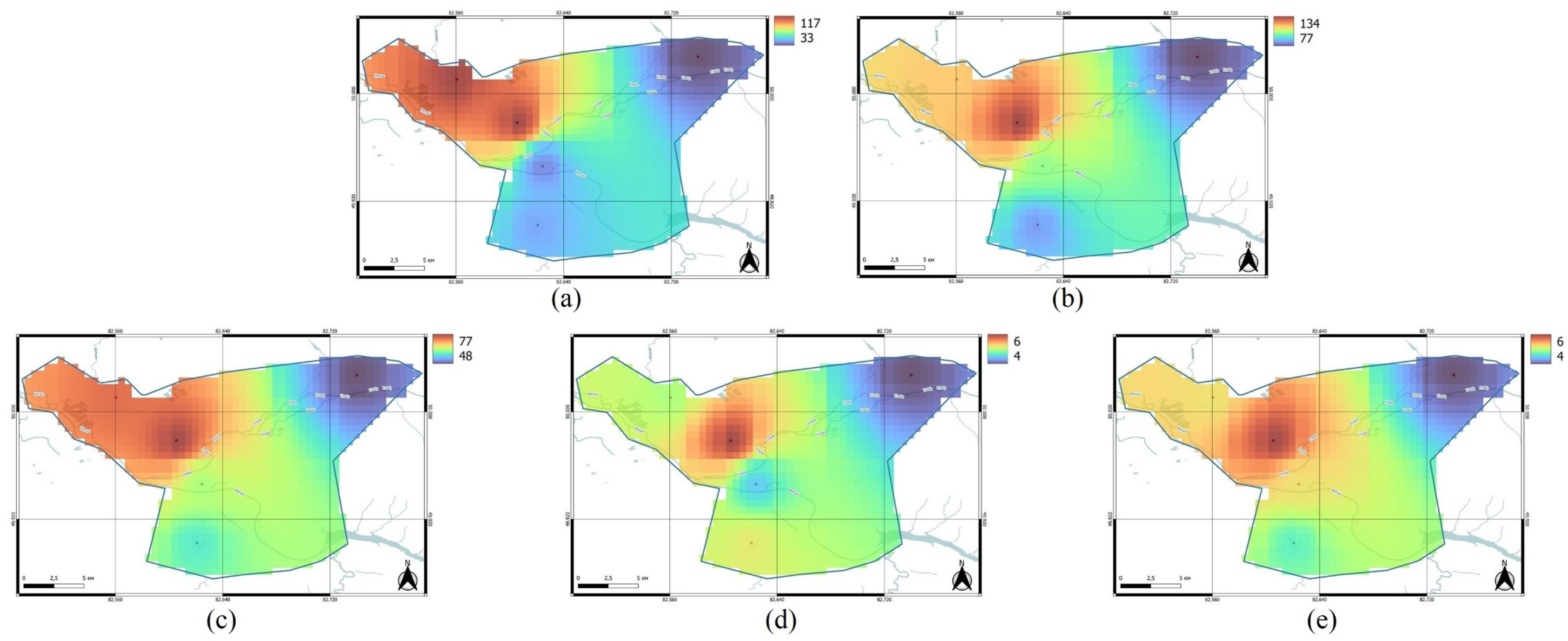
3. Results and Discussion

3.1. Hierarchical Clustering Analysis

Clustering analysis has been performed using dates as variables based on parameters of contamination to identify the similarities within particular periods. The final result of the analysis can be seen in Figure 2. The results indicate that the studied period can be grouped into two categories: cold (including months from September to March) and warm (from April to August) seasons. This can be explained by the fact that contaminants (except formaldehyde) have shown maximum concentrations during cold seasons with peaks during the months of December–February (Figure 3). Thus, the following assessment includes a separate analysis of air pollution patterns in both cold and warm seasons. These findings in seasonality can also be used in better planning for preparing for avoiding public health burdens during the seasons of interest [46].

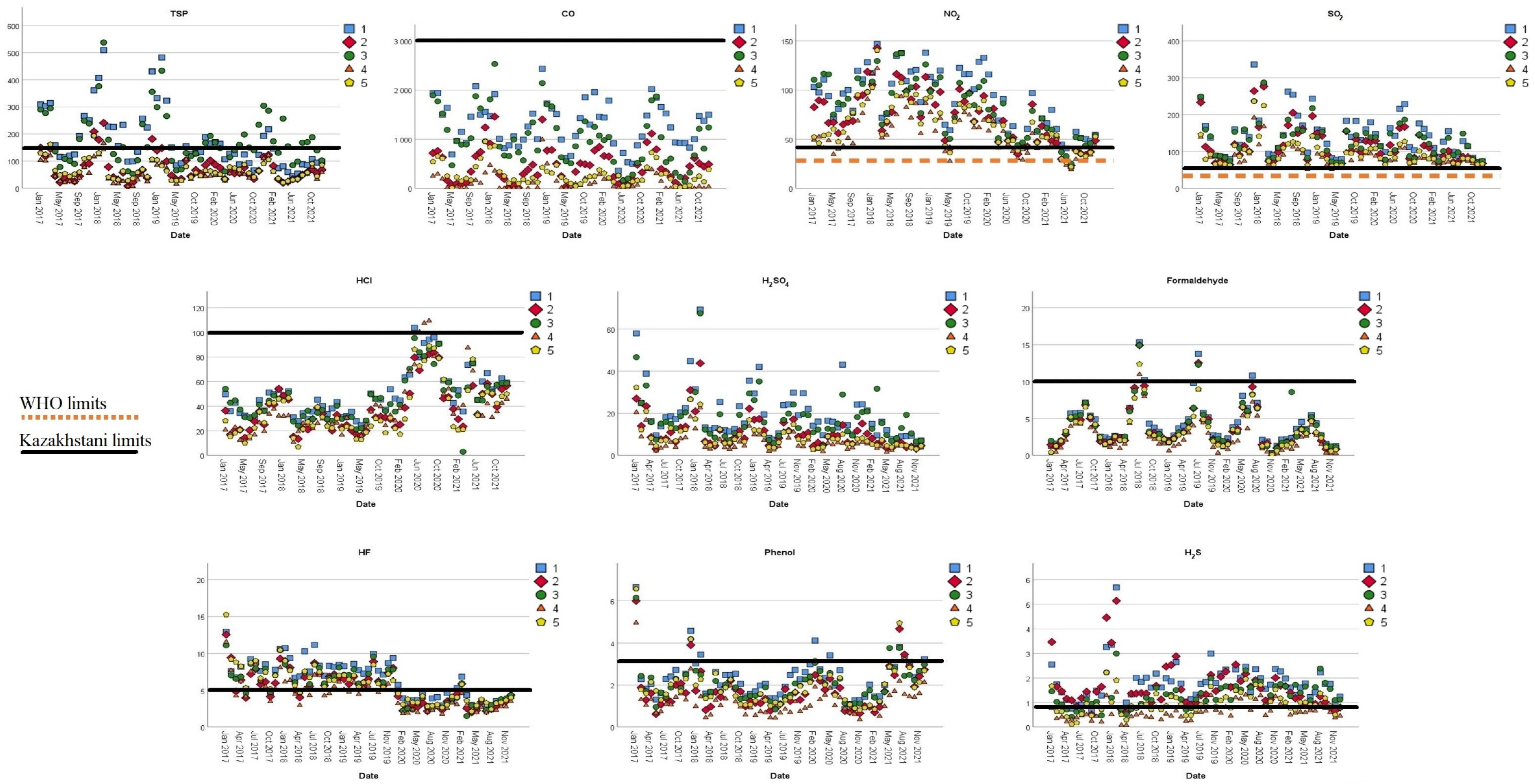
3.2. Descriptive Statistics

Table 2 and Table 3 present the results of measurements of air quality from the monitoring stations in the city according to the limits established by the Kazakhstani government and recommended by the WHO. It is clearly seen that heavy industry and coal-burnt energy cause the permanent exceeding of the permissible daily values along the city during both cold and warm seasons. The worst situation remains for NO₂ and SO₂, which are significantly higher than both limits (by 2–3 times for NO₂ and by 1.5–2 times for SO₂) during the whole period of analysis (Figure 3). Averaged concentrations of TSP slightly exceeded the established limits for Stations 1 and 3 during the cold seasons, with the peak values during January months in 2017 and 2018 (Figure 3), while during the warm seasons, they can be characterised as safe. Concentrations of HF and H₂S show slight excess over the recommended concentrations along all stations (except Station 4) during both seasons. However, the presence of HF dropped below the limit line after January 2020 (Figure 3). Surprisingly, the averaged and median concentrations of CO have not shown exceeding values, except several daily exceedings of the parameter were recognised during the cold seasons. In general, the concentrations of the pollutants show a slightly descending trend while they still remain much above the permissible level. It can be explained by the report from the National Statistics Committee, which claims that industrial emissions decreased from 29 to 27.9 kt/y for SO₂ and from 10.8 to 10.4 kt/y for CO for the period between 2017 and 2021 [47].

It is fair to note that the recently updated Kazakhstani limits [48] have not followed recommendations from international standards [49] and experts [50]. The limits for main pollutants have not been revised and still are above the recommendations from WHO [51].

The spatial distribution of the contaminants is presented in Figure 4 and Figure 5. Only TSP, SO₂, NO₂, HF, and formaldehyde show the most significant patterns in their dispersion within the city. It is clearly seen that the major emitter of the city is located near Station 1 and represents the northern industrial zone with two huge metallurgy factories and one thermal power plant. Surprisingly, the safest location in the city regarding concentrations of the pollutants is near Station 4, despite its close location to the northeastern industrial zone. The main difference between seasons is the presence of pollution near Station 5, in the southern direction from the major emitters to the downtown, which is located on the left-bank part of the city with its own thermal power plant. While concentrations of HF and formaldehyde look high, comparatively with the centre of the emissions during the cold seasons, the presence of these contaminants during the warm seasons looks safe and strives for minimal values within the city (Figure 4d,e and Figure 5d,e). Concentrations of SO₂ and NO₂ also do not show significant changes between the two seasons, with their decrease in the southern direction from Station 1 (Figure 4b,c and Figure 5b,c). The worst situation in a matter of TSP is in the northwestern part of the city near Stations 1 and 3 (Figure 4a and Figure 5a).

Table 2. Descriptive statistics of air quality during the cold seasons (in μg m⁻³).

	WHO Limits (Daily Averaged) [51]	Kazakhstani Limits (Daily Averaged) [48]		Station 1	Station 2	Station 3	Station 4	Station 5
TSP	-	150	Mean (SD)	217 (183)	94 (92)	218 (182)	68 (66)	81 (78)
			Median	175	75	175	50	50
			Range	0–1350	0–550	0–1250	0–425	0–550
SO2	40	50	Mean (SD)	150 (124)	122 (108)	134 (105)	88 (53)	101 (69)
			Median	100	84	93	73	79
			Range	31–1641	14–1738	31–1318	0–410	0–519
CO	4000	3000	Mean (SD)	1548 (877)	656 (686)	1285 (1025)	195 (371)	376 (483)
			Median	1500	500	1000	0	250
			Range	0–6250	0–3750	0–5750	0–2250	0–3500
NO2	25	40	Mean (SD)	96 (54)	77 (48)	86 (50)	61 (37)	69 (45)
			Median	85	68	75	53	58
			Range	0–380	5–315	0–362	5–323	0–365
Phenol	-	3	Mean (SD)	2.4 (1.8)	1.8 (1.6)	2.1 (1.7)	1.2 (1.4)	1.9 (1.7)
			Median	2.0	1.5	1.8	0.8	1.5
			Range	0–12.8	0–11.0	0–20.5	0–20.5	0–16.0
HF	-	5	Mean (SD)	6.6 (3.5)	5.6 (3.4)	5.8 (3.4)	4.6 (3.0)	5.9 (3.8)
			Median	6.3	5.0	5.3	4.0	5.3
			Range	0–25	0–25	0–25	0–18	0–29
HCl	-	100	Mean (SD)	49.2 (28.5)	37.1 (28.5)	45.5 (27.5)	35.2 (28.6)	34.9 (29)
			Median	50.0	30.0	47.5	30.0	30.0
			Range	0–175.0	0–142.5	0–152.5	0–142.5	0–145
H2SO4	-	100	Mean (SD)	23.2 (25.4)	12.5 (15.4)	20.6 (22.1)	7.6 (10.0)	10.2 (12.7)
			Median	15.0	7.5	15.0	5.0	7.5
			Range	0–280.0	0–157.5	0–220.0	0–165.0	0–172.5
Formaldehyde	-	10	Mean (SD)	2.6 (2.0)	2.2 (1.8)	2.5 (2.2)	1.3 (1.6)	2.1 (1.9)
			Median	2.5	1.5	2.5	1.3	2.0
			Range	0–11.8	0–10.0	0–15.0	0–10.0	0–11.8
H2S	-	0.8	Mean (SD)	2.0 (1.8)	1.8 (2.1)	1.4 (1.1)	0.6 (0.7)	1.0 (1.0)
			Median	1.5	1.3	1.0	0.5	1.0
			Range	0–18.3	0–23.0	0–11.8	0–5.0	0–11.8

Table 2. Descriptive statistics of air quality during the cold seasons (in μg m⁻³).

	WHO Limits (Daily Averaged) [51]	Kazakhstani Limits (Daily Averaged) [48]		Station 1	Station 2	Station 3	Station 4	Station 5
TSP	-	150	Mean (SD)	217 (183)	94 (92)	218 (182)	68 (66)	81 (78)
			Median	175	75	175	50	50
			Range	0–1350	0–550	0–1250	0–425	0–550
SO2	40	50	Mean (SD)	150 (124)	122 (108)	134 (105)	88 (53)	101 (69)
			Median	100	84	93	73	79
			Range	31–1641	14–1738	31–1318	0–410	0–519
CO	4000	3000	Mean (SD)	1548 (877)	656 (686)	1285 (1025)	195 (371)	376 (483)
			Median	1500	500	1000	0	250
			Range	0–6250	0–3750	0–5750	0–2250	0–3500
NO2	25	40	Mean (SD)	96 (54)	77 (48)	86 (50)	61 (37)	69 (45)
			Median	85	68	75	53	58
			Range	0–380	5–315	0–362	5–323	0–365
Phenol	-	3	Mean (SD)	2.4 (1.8)	1.8 (1.6)	2.1 (1.7)	1.2 (1.4)	1.9 (1.7)
			Median	2.0	1.5	1.8	0.8	1.5
			Range	0–12.8	0–11.0	0–20.5	0–20.5	0–16.0
HF	-	5	Mean (SD)	6.6 (3.5)	5.6 (3.4)	5.8 (3.4)	4.6 (3.0)	5.9 (3.8)
			Median	6.3	5.0	5.3	4.0	5.3
			Range	0–25	0–25	0–25	0–18	0–29
HCl	-	100	Mean (SD)	49.2 (28.5)	37.1 (28.5)	45.5 (27.5)	35.2 (28.6)	34.9 (29)
			Median	50.0	30.0	47.5	30.0	30.0
			Range	0–175.0	0–142.5	0–152.5	0–142.5	0–145
H2SO4	-	100	Mean (SD)	23.2 (25.4)	12.5 (15.4)	20.6 (22.1)	7.6 (10.0)	10.2 (12.7)
			Median	15.0	7.5	15.0	5.0	7.5
			Range	0–280.0	0–157.5	0–220.0	0–165.0	0–172.5
Formaldehyde	-	10	Mean (SD)	2.6 (2.0)	2.2 (1.8)	2.5 (2.2)	1.3 (1.6)	2.1 (1.9)
			Median	2.5	1.5	2.5	1.3	2.0
			Range	0–11.8	0–10.0	0–15.0	0–10.0	0–11.8
H2S	-	0.8	Mean (SD)	2.0 (1.8)	1.8 (2.1)	1.4 (1.1)	0.6 (0.7)	1.0 (1.0)
			Median	1.5	1.3	1.0	0.5	1.0
			Range	0–18.3	0–23.0	0–11.8	0–5.0	0–11.8

Table 3. Descriptive statistics of air quality during the warm seasons (μg m⁻³).

	WHO Limits (Daily Averaged) [51]	Kazakhstani Limits (Daily Averaged) [48]		Station 1	Station 2	Station 3	Station 4	Station 5
TSP	-	150	Mean (SD)	118 (81)	41 (42)	117 (80)	33 (41)	47 (45)
			Median	100	25	100	25	25
			Range	0–500	0–375	0–475	0–375	0–300
SO2	40	50	Mean (SD)	135 (98)	102 (63)	116 (68)	77 (30)	85 (36)
			Median	98	81	90	71	75
			Range	45–1100	13–490	43–468	13–256	0–353
CO	4000	3000	Mean (SD)	886 (607)	149 (234)	571 (517)	19 (107)	133 (219)
			Median	750	0	500	0	0
			Range	0–5000	0–1750	0–2750	0–1250	0–1250
NO2	25	40	Mean (SD)	78 (46)	62 (38)	74 (43)	48 (29)	58 (35)
			Median	70	54	68	45	53
			Range	0–308	0–212	0–233	0–218	0–263
Phenol	-	3	Mean (SD)	2.2 (1.6)	1.8 (1.6)	2.0 (1.5)	1.2 (1.1)	2.0 (1.7)
			Median	2.0	1.5	1.8	0.8	1.8
			Range	0–16.5	0–18.0	0–17.0	0–5.5	0–14.8
HF	-	5	Mean (SD)	6.2 (3.6)	4.9 (3.1)	5.3 (3.1)	4.5 (3.0)	5.5 (3.3)
			Median	6.0	4.3	5.0	3.5	4.9
			Range	0–20.0	0–16.3	0–16.5	0–15.5	0–16.3
HCl	-	100	Mean (SD)	51 (34)	39 (32)	48 (32)	42 (39)	39 (34)
			Median	48	33	45	30	30
			Range	0–167	0–175	0–148	0–173	0–145
H2SO4	-	100	Mean (SD)	14.6 (15.7)	7.5 (6.4)	12.1 (9.6)	4.4 (4.4)	6.9 (5.0)
			Median	12.5	7.5000	10.0	2.5	5.0
			Range	0–222.5	0–52.5	0–102.5	0–30.0	0–33.0
Formaldehyde	-	10	Mean (SD)	6.8 (5.0)	5.9 (4.7)	5.9 (4.3)	4.5 (3.4)	5.3 (3.6)
			Median	5.9	4.8	5.0	3.8	4.5
			Range	0–33.5	0–35.8	0–32.3	0–21.8	0–28.0
H2S	-	0.8	Mean (SD)	1.5 (0.9)	1.3 (0.8)	1.2 (0.9)	0.6 (0.6)	0.9 (0.8)
			Median	1.5	1.0	1.0	0.5	0.8
			Range	0–5.5	0–4.3	0–4.8	0–3.5	0–3.8

Table 3. Descriptive statistics of air quality during the warm seasons (μg m⁻³).

	WHO Limits (Daily Averaged) [51]	Kazakhstani Limits (Daily Averaged) [48]		Station 1	Station 2	Station 3	Station 4	Station 5
TSP	-	150	Mean (SD)	118 (81)	41 (42)	117 (80)	33 (41)	47 (45)
			Median	100	25	100	25	25
			Range	0–500	0–375	0–475	0–375	0–300
SO2	40	50	Mean (SD)	135 (98)	102 (63)	116 (68)	77 (30)	85 (36)
			Median	98	81	90	71	75
			Range	45–1100	13–490	43–468	13–256	0–353
CO	4000	3000	Mean (SD)	886 (607)	149 (234)	571 (517)	19 (107)	133 (219)
			Median	750	0	500	0	0
			Range	0–5000	0–1750	0–2750	0–1250	0–1250
NO2	25	40	Mean (SD)	78 (46)	62 (38)	74 (43)	48 (29)	58 (35)
			Median	70	54	68	45	53
			Range	0–308	0–212	0–233	0–218	0–263
Phenol	-	3	Mean (SD)	2.2 (1.6)	1.8 (1.6)	2.0 (1.5)	1.2 (1.1)	2.0 (1.7)
			Median	2.0	1.5	1.8	0.8	1.8
			Range	0–16.5	0–18.0	0–17.0	0–5.5	0–14.8
HF	-	5	Mean (SD)	6.2 (3.6)	4.9 (3.1)	5.3 (3.1)	4.5 (3.0)	5.5 (3.3)
			Median	6.0	4.3	5.0	3.5	4.9
			Range	0–20.0	0–16.3	0–16.5	0–15.5	0–16.3
HCl	-	100	Mean (SD)	51 (34)	39 (32)	48 (32)	42 (39)	39 (34)
			Median	48	33	45	30	30
			Range	0–167	0–175	0–148	0–173	0–145
H2SO4	-	100	Mean (SD)	14.6 (15.7)	7.5 (6.4)	12.1 (9.6)	4.4 (4.4)	6.9 (5.0)
			Median	12.5	7.5000	10.0	2.5	5.0
			Range	0–222.5	0–52.5	0–102.5	0–30.0	0–33.0
Formaldehyde	-	10	Mean (SD)	6.8 (5.0)	5.9 (4.7)	5.9 (4.3)	4.5 (3.4)	5.3 (3.6)
			Median	5.9	4.8	5.0	3.8	4.5
			Range	0–33.5	0–35.8	0–32.3	0–21.8	0–28.0
H2S	-	0.8	Mean (SD)	1.5 (0.9)	1.3 (0.8)	1.2 (0.9)	0.6 (0.6)	0.9 (0.8)
			Median	1.5	1.0	1.0	0.5	0.8
			Range	0–5.5	0–4.3	0–4.8	0–3.5	0–3.8

3.3. Principal Component Analysis

The correlation matrix was employed for each monitoring station for all 859 and 602 measurements (for cold and warm seasons, respectively) for determining relationships: in particular, pairs between contaminants and meteorological parameters. Figure 6 shows the averaged values for correlation coefficients among the monitoring stations. The analysis has not identified any correlation between the chemical and meteorological (including wind direction, wind speed, relative humidity, and temperature) parameters.

Table 4. Principal Component Analysis for the cold seasons.

	Station 1		Station 2		Station 3			Station 4			Station 5
	PC1	PC2	PC1	PC2	PC1	PC2	PC3	PC1	PC2	PC3	PC1	PC2	PC3
TSP	0.803	0.093	0.859	−0.121	0.829	0.228	0.079	0.773	0.218	−0.047	0.669	0.509	0.109
SO2	0.841	−0.054	0.835	−0.018	0.745	0.395	0.007	0.747	0.363	0.150	0.603	0.476	0.350
CO	0.633	−0.023	0.796	−0.267	0.800	0.237	0.065	0.718	0.068	0.015	0.681	0.387	−0.001
NO2	0.748	0.198	0.772	0.197	0.580	0.485	−0.216	0.523	0.260	0.465	0.406	0.315	0.573
Phenol	0.530	0.035	0.452	−0.036	0.146	0.686	0.197	0.212	0.590	−0.234	0.066	0.748	−0.133
HF	0.560	0.443	0.545	0.340	0.232	0.776	−0.078	0.304	0.671	0.172	0.107	0.763	0.159
HCl	0.248	−0.758	0.225	−0.650	0.361	−0.155	0.684	0.493	−0.584	−0.138	0.693	−0.317	−0.125
H2SO4	0.835	−0.060	0.809	−0.046	0.804	0.197	−0.045	0.695	0.348	0.009	0.467	0.580	0.180
Formaldehyde	0.101	0.558	0.092	0.747	0.175	−0.199	−0.788	−0.011	−0.050	0.893	−0.095	−0.086	0.880
H2S	0.739	−0.220	0.806	−0.100	0.706	−0.018	0.109	0.708	−0.102	0.059	0.702	0.164	0.090
Eigenvalue	4.223	1.185	4.541	1.222	3.599	1.675	1.205	3.309	1.526	1.146	2.656	2.346	1.336
% of variance	42.231	11.847	45.409	12.223	35.986	16.751	12.049	33.089	15.264	11.457	26.559	23.465	13.363
Cumulative %	42.231	54.078	45.409	57.632	35.986	52.738	64.787	33.089	48.352	59.809	26.559	50.024	63.387

and

Table 5. Principal Component Analysis for the warm seasons.

	Station 1				Station 2			Station 3			Station 4			Station 5
	PC1	PC2	PC3	PC4	PC1	PC2	PC3	PC1	PC2	PC3	PC1	PC2	PC3	PC1	PC2	PC3
TSP	0.087	0.321	0.665	−0.130	0.210	0.026	0.664	0.119	−0.107	0.838	0.150	0.427	0.548	0.209	0.200	0.684
SO2	0.711	0.278	−0.044	−0.008	0.679	0.303	0.127	0.502	0.569	0.230	0.717	0.336	0.006	0.685	0.399	0.124
CO	−0.113	0.023	0.804	0.143	−0.195	0.032	0.725	−0.519	0.339	0.521	0.185	−0.014	0.393	−0.066	−0.206	0.776
NO2	0.187	0.751	0.303	0.094	0.727	−0.335	0.107	−0.276	0.744	0.158	0.679	−0.200	0.063	0.699	−0.280	0.059
Phenol	0.179	−0.073	0.097	0.865	−0.044	0.413	−0.045	0.359	−0.001	−0.158	0.318	0.299	−0.666	0.005	0.376	−0.165
HF	−0.179	0.773	0.155	−0.166	0.474	−0.637	0.057	−0.522	0.588	−0.114	0.521	−0.538	0.193	0.436	−0.618	0.007
HCl	0.645	−0.484	0.054	0.054	0.099	0.757	0.220	0.691	−0.087	0.273	−0.045	0.806	0.121	0.038	0.779	0.134
H2SO4	0.458	−0.031	0.421	−0.497	0.261	0.050	0.626	0.112	0.206	0.693	0.411	0.154	0.399	0.450	0.095	0.476
Formaldehyde	0.485	0.612	−0.088	0.002	0.825	−0.035	0.067	0.197	0.820	0.008	0.787	0.076	0.120	0.797	0.098	0.081
H2S	0.763	0.005	0.012	0.111	0.425	0.516	0.111	0.734	0.078	0.190	0.152	0.704	−0.063	0.228	0.684	0.119
Eigenvalue	2.069	1.958	1.404	1.085	2.238	1.626	1.457	2.078	2.078	1.680	2.218	1.888	1.132	2.087	1.936	1.382
% of variance	20.693	19.578	14.037	10.850	22.377	16.260	14.567	20.779	20.778	16.797	22.177	18.880	11.325	20.872	19.360	13.817
Cumulative %	20.693	40.271	54.308	65.158	22.377	38.637	53.205	20.779	41.557	58.354	22.177	41.056	52.381	20.872	40.232	54.049

, representing the principal components (PCs), have been developed for contaminants measurements only to identify groups of the contaminants, which can be combined by their common origin or specific properties of their spatiotemporal distribution (

Table 6. Grouped PCs for cold and warm seasons.

Cold Season		Warm Season
Group 1	Group 2	Group 1	Group 2
TSP	HCl	SO2	TSP
SO2	Formaldehyde	NO2	CO
CO		Formaldehyde	Phenol
NO2		HCl	H2SO4
Phenol		H2S
HF		HF
H2SO4
H2S

). Bold values in Table 4 and Table 5 denote high loadings of the contaminants to the calculated PCs. The eigenvalues of the identified PCs are all greater than 1.0, and according to the Kaiser criterion, these PCs have to be chosen [52]. The results did not show significant differences between the stations in general, which may indicate a relatively equal distribution of pollution within the city. Particular differences are described in the subsections for each PC below. It is important to note here that the correlation during the cold seasons is stronger than during the warm seasons (Figure 6). Two PCs have been identified for the cold season analysis for the monitoring Stations 1 and 2, while three PCs have been identified for other monitoring stations. Therefore, included parameters in PCs 1 and 2 for Stations 3–5 are almost the same as the parameters included in PC1 for Stations 1–2. PCA, for the warm season, has identified three PCs for Stations 2–5 and four PCs for Station 1.

3.3.1. PC1

PC1 of the cold season is characterised by high positive weight values for TSP, SO₂, CO, and H₂S for every monitoring station. NO₂, phenol, HF, and H₂SO₄ may also be conditionally added to the list, as they have been formulated as PC 1 for Stations 1, 2, 3, and 4 and have been included in PC2 for Station 5. Altogether, the PC1 for Stations 1–2 and PC1 + PC2 for Stations 3–5 explain 47.7% of the total variance on average. As Figure 6 indicates, there is a strong positive correlation between TSP, SO₂, CO, and H₂S. NO₂ and H₂SO₄ also show a significant correlation with the listed contaminants. These ions are the major contributors to the total suspended particles. Additionally, these ions correlate with each other. It can be concluded that these contaminants have a shared source of their origin. The results of the appearance of TSP and CO in one group with SO₂ and NO₂ for the cold seasons and theirs separating for the warm seasons can be well explained by the fact that SO₂ and NO₂ are emitted mainly from combustion processes, while the sources for TSP are far more (for example, wind-driven and traffic-related re-suspension and biogenic sources) [53]. In addition, the metallurgy sector, which prevails in Ust-Kamenogorsk among emitters, can be characterised as the major source of SO₂ [54] and TSP (on behalf of PM_2.5) [55]. It is well known that the exposure of TSP-sulphur-derived contaminants in the air is believed to be representative of emissions from the combustion of fossil fuels, which increases the risk for bronchitis and some other respiratory disorders [56]. In addition, it is worth mentioning that nitrogen dioxide has been listed as an emerging pollutant causing morbidity and mortality [57].

PC1 of the warm season seems more uncertain, as there are no contaminants repeated in each of the monitoring stations. SO₂ (in four of five monitoring stations) and NO₂ and formaldehyde (in three of five) have been identified in PC1 as the most common contaminants. The contaminants SO₂, NO₂, and formaldehyde have been the same for the monitoring Stations 2, 4, and 5. This combination of the stations and the identified contaminants can be explained by the proximity of the monitoring stations to heat supply sources and highways [58] and the respective photochemical reactions in the atmosphere nearby [59]. In addition, the contaminants HCl and H₂S have been identified as key contaminants in PC1 for Stations 1 and 3, which can be explained by emissions from the largest thermal power plant. A study [60] says that H₂S is formed by the combustion of coal with high content of sulphur, which is an exact characteristic of Kazakhstani coal. The loading of HCl within this PC can be explained by the emissions from Kazzinc LLP according to the technological scheme of the enterprise.

3.3.2. PC2

PC2 in warm seasons compensates for the above-mentioned contaminants in the stations which previously have not been listed as belonging to PC1. For example, for Stations 2, 4, and 5, the list of contaminants includes HCl and H₂S. As mentioned above, the source of HCl emissions can be the metallurgy industry, which uses acid for production purposes. H2S can be emitted due to coal combustion. Station 2 is located in the central part of the city at a considerable distance from industrial facilities. However, sources of emissions located at a reasonable elevation can disperse HCl and H₂S to the centre of the city. For Stations 4 and 5, the presence of the parameters in this PC can be explained by the proximity of the northeastern industrial zone and the Sogrinskaya and the left-bank thermal power plants.

For Stations 1 and 3, the list of contaminants has been fulfilled by SO₂, NO₂, and formaldehyde. The northern industrial zone is a dominant emitter for Station 3, which can easily explain the presence of SO₂ and NO₂ in this PC. HF has been identified as the key contaminant for this PC in four of five monitoring stations. Figure 4 and Figure 5 show that HF is mainly concentrated in the area of the northern industrial zone and then is evenly distributed throughout the city during both the cold and warm seasons. The thermal power plants do not monitor the concentrations of HF in their emissions, while there are a number of research [61,62] and official reports [63,64] showing the coal-fired stations as the largest anthropogenic sources of HF. The situation for formaldehyde looks the same as for HF. No enterprises monitor this chemical, while the direction of spatial distribution shows a similar direction.

3.3.3. PC3

PC3, for the warm season, has grouped TPS and CO, which indicates their shared source of origin, even though there is no household heating during the comfortable weather conditions and emissions from the central heating are expected to be minimal. Moreover, it is expected that nature might neglect the effect of air pollution by these contaminants, which seems to be a reason for such difference in the rate of these contaminants in the cold (the most impactful contaminants) and warm (the least impactful contaminants) seasons. In addition, phenol (in Stations 1 and 4) and H₂SO₄ (in Stations 2 and 3) have been revealed as belonging to this PC. Sulphuric acid is actively used in metallurgy, and this parameter shows the shared source in this PC with TPS and CO. The appearance of phenol in this PC requires additional studies, as its spread is unusual for metallurgy. This PC can be explained by a geographical location, as it focuses on the air conditions in the central part of the city. While emissions can be dispersed from the northern industrial zone according to Figure 4 and Figure 5, the presence of phenol can be explained by intensive traffic [65].

Table 6 summarises a conditional grouping of identified PCs, results of the spatiotemporal assessment, hierarchical clustering analysis, and respective chemicals. Group 1 for the cold seasons can be explained by the intensive use of the fossil fuel fired by all users: power plants, industry, and households coupled with meteorological conditions (based on Figure 6). This mix ensures a variety of pollutants are released into the atmosphere by the burning of different types of fuel. The same group for the warm seasons indicates and highlights the problem of coal consumption, mainly by industrial enterprises, which is indicated by the uniform seasonal distribution of NO₂ and SO₂ [4]. Group 2 for the cold seasons can be explained by specific industrial processes and the release of the associated contaminants into the atmosphere. Group 2 for the warm seasons could indicate a contribution of traffic to air pollution. While local authorities have attempted to explain air quality issues by a high density of motor transport, the results of this study confirm outcomes of previous research on heavy air pollution in the city caused by non-transport-related sources [66]: that this factor has a low significance comparatively with the impact of industrial activities, especially burnt-coal based.

4. Conclusions

Ust-Kamenogorsk is one of the most important industrial centres of Kazakhstan, where non-ferrous metals are produced and exported abroad for the largest world companies. The active consumption of coal and raw material orientation of the industrial enterprises makes Ust-Kamenogorsk one of the most polluted industrial cities in the world. This study, for the first time, aimed to analyse spatiotemporal patterns of air pollution in the city and to identify potential sources of apportionment using multivariate statistical techniques. The results show that the combination of large enterprises and coal-fired thermal power plants severely affects air quality in Ust-Kamenogorsk. The average concentrations of SO₂ and NO₂ for the entire study period exceeded the standards of WHO and Kazakhstan within the whole city all year round. The major emitters are located in the northern industrial zone with two huge metallurgy factories and one thermal power plant. The Principal Component Analysis revealed that emissions of TSP, SO₂, CO, H₂S, NO₂, HF, and H₂SO₄ with high likelihood are of industrial origin, which is significantly aggravated during the cold seasons. While official reports show a decrease in industrial emissions, air quality has not been improved even during the warm seasons when households stop heating with the expected elimination of air pollution.

The results of this study can be valuable for decision-makers in developing and applying respective strategies and actions for a decrease in air pollution and elimination of the social and environmental effects. The main limitation of the research is the difficulty in determining the ratio of the contributions of the major emitters to the high level of air pollution. Future research will focus on a detailed investigation of the composition of unstudied contaminants (particularly, particulate matters) in both ambient air and the zones of industrial enterprises. This research should be combined with the modelling of source profiles or fingerprints.

The air quality issues in Ust-Kamenogorsk most probably have been caused by a combination of the factors: weak environmental regulation and control, the influence of large companies on the legislative process through large professional associations, and an outdated and energy-intensive industry. The authors hope that the outcomes of this and other studies would be a sufficient research basis for authorities to develop the right strategy for air management in the region.

References

1. IQAir.com. World’s Most Polluted Countries 2020 (PM2.5). Available online: https://www.iqair.com/world-most-polluted-countries (accessed on 23 August 2022).
2. Zhu, L.; Hao, Y.; Lu, Z.-N.; Wu, H.; Ran, Q. Do economic activities cause air pollution? Evidence from China’s major cities. Sustain. Cities Soc. 2019, 49, 101593. [Google Scholar] [CrossRef]
3. Yuan, M.; Song, Y.; Huang, Y.; Hong, S.; Huang, L. Exploring the Association between Urban Form and Air Quality in China. J. Plan. Educ. Res. 2017, 38, 413–426. [Google Scholar] [CrossRef]
4. Zhao, Y.; Qiu, L.P.; Xu, R.Y.; Xie, F.J.; Zhang, Q.; Yu, Y.Y.; Nielsen, C.P.; Qin, H.X.; Wang, H.K.; Wu, X.C.; et al. Advantages of a city-scale emission inventory for urban air quality research and policy: The case of Nanjing, a typical industrial city in the Yangtze River Delta, China. Atmos. Chem. Phys. 2015, 15, 12623–12644. [Google Scholar] [CrossRef] [Green Version]
5. Gu, Y.; Wong, T.W.; Law, C.; Dong, G.H.; Ho, K.F.; Yang, Y.; Yim, S.H.L. Impacts of sectoral emissions in China and the implications: Air quality, public health, crop production, and economic costs. Environ. Res. Lett. 2018, 13, 084008. [Google Scholar] [CrossRef]
6. Burnett, R.; Chen, H.; Szyszkowicz, M.; Fann, N.; Hubbell, B.; Pope, C.A.; Apte, J.S.; Brauer, M.; Cohen, A.; Weichenthal, S.; et al. Global estimates of mortality associated with long-term exposure to outdoor fine particulate matter. Proc. Natl. Acad. Sci. USA 2018, 115, 9592–9597. [Google Scholar] [CrossRef] [Green Version]
7. Assanov, D.A.; Filyanova, L.A.; Zapasnyi, V.V.; Sukhova, N.M. Study of the Performance Indices of a Dust-Cleaning System at the Balkhash Copper Smelter. Metallurgist 2016, 60, 331–338. [Google Scholar] [CrossRef]
8. Assanov, D.A.; Zapasnyi, V.V.; Ermekova, A.T.; Maratova, G.R.; Ivanov, A.A.; Cherepanov, N.I. Current Status of Dust Collection Systems in Aksu Ferroalloy Plant Smelting Shop 1 and Functional Improvement to These Systems. Metallurgist 2018, 62, 391–400. [Google Scholar] [CrossRef]
9. Assanov, D.; Zapasnyi, V.; Kerimray, A. Air Quality and Industrial Emissions in the Cities of Kazakhstan. Atmosphere 2021, 12, 314. [Google Scholar] [CrossRef]
10. Abdildin, Y.G.; Nurkenov, S.A.; Kerimray, A. Analysis of Green Technology Development in Kazakhstan. Int. J. Energy Econ. Policy 2021, 11, 269–279. [Google Scholar] [CrossRef]
11. Russell, A.; Ghalaieny, M.; Gazdiyeva, B.; Zhumabayeva, S.; Kurmanbayeva, A.; Akhmetov, K.K.; Mukanov, Y.; McCann, M.; Ali, M.; Tucker, A.; et al. A Spatial Survey of Environmental Indicators for Kazakhstan: An Examination of Current Conditions and Future Needs. Int. J. Environ. Res. 2018, 12, 735–748. [Google Scholar] [CrossRef]
12. Kerimray, A.; Assanov, D.; Kenessov, B.; Karaca, F. Trends and health impacts of major urban air pollutants in Kazakhstan. J. Air Waste Manag. 2020, 70, 1148–1164. [Google Scholar] [CrossRef] [PubMed]
13. Baimatova, N.; Omarova, A.; Muratuly, A.; Tursumbayeva, M.; Ibragimova, O.P.; Bukenov, B.; Kerimray, A. Seasonal Variations and Effect of COVID-19 Lockdown Restrictions on the Air Quality in the Cities of Kazakhstan. Environ. Process. 2022, 9, 48. [Google Scholar] [CrossRef]
14. Zlatev, V.; Cofala, J.; Peszko, G.; Wang, Q. Clean Air and Cool Planet—Cost-Effective Air Quality Management in Kazakhstan and Its Impact on Greenhouse Gas Emissions; The World Bank: Washington, DC, USA, 2021. [Google Scholar]
15. Informburo. Pink Smoke Pours from the Pipes of the Titanium-Magnesium Plant in Ust-Kamenogorsk. 2021. Available online: https://informburo.kz/novosti/iz-trub-titano-magnievogo-kombinata-v-ust-kamenogorske-valit-rozovyi-dym (accessed on 29 October 2022).
16. Assanov, D.; Kerimray, A.; Batkeyev, B.; Kapsalyamova, Z. The Effects of COVID-19-related Driving Restrictions on Air Quality in an Industrial City. Aerosol Air Qual. Res. 2021, 21, 200663. [Google Scholar] [CrossRef]
17. Semenova, Y.; Zhunussov, Y.; Pivina, L.; Abisheva, A.; Tinkov, A.; Belikhina, T.; Skalny, A.; Zhanaspayev, M.; Bulegenov, T.; Glushkova, N.; et al. Trace element biomonitoring in hair and blood of occupationally unexposed population residing in polluted areas of East Kazakhstan and Pavlodar regions. J. Trace Elem. Med. Biol. 2019, 56, 31–37. [Google Scholar] [CrossRef] [PubMed]
18. Miranda, A.; Silveira, C.; Ferreira, J.; Monteiro, A.; Lopes, D.; Relvas, H.; Borrego, C.; Roebeling, P. Current air quality plans in Europe designed to support air quality management policies. Atmos. Pollut. Res. 2015, 6, 434–443. [Google Scholar] [CrossRef] [Green Version]
19. Gulia, S.; Shiva Nagendra, S.M.; Khare, M.; Khanna, I. Urban air quality management—A review. Atmos. Pollut. Res. 2015, 6, 286–304. [Google Scholar] [CrossRef] [Green Version]
20. Wang, K.; Yin, H.; Chen, Y. The effect of environmental regulation on air quality: A study of new ambient air quality standards in China. J. Clean. Prod. 2019, 215, 268–279. [Google Scholar] [CrossRef]
21. Jiang, L.; Zhou, H.-F.; Bai, L.; Zhou, P. Does foreign direct investment drive environmental degradation in China? An empirical study based on air quality index from a spatial perspective. J. Clean. Prod. 2018, 176, 864–872. [Google Scholar] [CrossRef]
22. Mir, K.A.; Purohit, P.; Cail, S.; Kim, S. Co-benefits of air pollution control and climate change mitigation strategies in Pakistan. Environ. Sci. Policy 2022, 133, 31–43. [Google Scholar] [CrossRef]
23. Chen, B.; Cheng, Y. The Impacts of Environmental Regulation on Industrial Activities: Evidence from a Quasi-Natural Experiment in Chinese Prefectures. Sustainability 2017, 9, 571. [Google Scholar] [CrossRef]
24. Pui, D.Y.H.; Chen, S.-C.; Zuo, Z. PM2.5 in China: Measurements, sources, visibility and health effects, and mitigation. Particuology 2014, 13, 1–26. [Google Scholar] [CrossRef]
25. Belis, C.A.; Larsen, B.R.; Amato, F.; El Haddad, I.; Favez, O.; Harrison, R.M.; Hopke, P.K.; Nava, S.; Paatero, P.; Prevot, A. European Guide on Air Pollution Source Apportionment with Receptor Models; Publications Office of the European Union: Luxembourg, 2019. [Google Scholar]
26. Schichtel, B.A.; Malm, W.C.; Gebhart, K.A.; Barna, M.G.; Knipping, E.M. A hybrid source apportionment model integrating measured data and air quality model results. J. Geophys. Res.: Atmos. 2006, 111, D07301. [Google Scholar] [CrossRef] [Green Version]
27. Dai, H.; Huang, G.; Wang, J.; Zeng, H.; Zhou, F. Prediction of Air Pollutant Concentration Based on One-Dimensional Multi-Scale CNN-LSTM Considering Spatial-Temporal Characteristics: A Case Study of Xi’an, China. Atmosphere 2021, 12, 1626. [Google Scholar] [CrossRef]
28. Belis, C.A.; Karagulian, F.; Larsen, B.R.; Hopke, P.K. Critical review and meta-analysis of ambient particulate matter source apportionment using receptor models in Europe. Atmos. Environ. 2013, 69, 94–108. [Google Scholar] [CrossRef]
29. Lee, C.L.; Jie, W.Y.; Arumugasamy, S.K. Dynamic simulation of airborne pollutant concentrations associated with the effect of climate change in Batu Muda region, Malaysia. Model. Earth Syst. Environ. 2022, 8, 323–338. [Google Scholar] [CrossRef]
30. Jeričević, A.; Gašparac, G.; Mikulec, M.M.; Kumar, P.; Prtenjak, M.T. Identification of diverse air pollution sources in a complex urban area of Croatia. J. Environ. Manag. 2019, 243, 67–77. [Google Scholar] [CrossRef]
31. Kousehlar, M.; Widom, E. Identifying the sources of air pollution in an urban-industrial setting by lichen biomonitoring—A multi-tracer approach. Appl. Geochem. 2020, 121, 104695. [Google Scholar] [CrossRef]
32. Kumar, P.; Morawska, L.; Martani, C.; Biskos, G.; Neophytou, M.; Di Sabatino, S.; Bell, M.; Norford, L.; Britter, R. The rise of low-cost sensing for managing air pollution in cities. Environ. Int. 2015, 75, 199–205. [Google Scholar] [CrossRef] [Green Version]
33. Pérez-Arribas, L.V.; León-González, M.E.; Rosales-Conrado, N. Learning Principal Component Analysis by Using Data from Air Quality Networks. J. Chem. Educ. 2017, 94, 458–464. [Google Scholar] [CrossRef]
34. Dominick, D.; Juahir, H.; Latif, M.T.; Zain, S.M.; Aris, A.Z. Spatial assessment of air quality patterns in Malaysia using multivariate analysis. Atmos. Environ. 2012, 60, 172–181. [Google Scholar] [CrossRef]
35. Kassomenos, P.A.; Kelessis, A.; Paschalidou, A.K.; Petrakakis, M. Identification of sources and processes affecting particulate pollution in Thessaloniki, Greece. Atmos. Environ. 2011, 45, 7293–7300. [Google Scholar] [CrossRef]
36. Khare, P.; Baruah, B.P. Elemental characterization and source identification of PM2.5 using multivariate analysis at the suburban site of North-East India. Atmos. Res. 2010, 98, 148–162. [Google Scholar] [CrossRef]
37. Azid, A.; Juahir, H.; Toriman, M.E.; Kamarudin, M.K.A.; Saudi, A.S.M.; Hasnam, C.N.C.; Aziz, N.A.A.; Azaman, F.; Latif, M.T.; Zainuddin, S.F.M.; et al. Prediction of the Level of Air Pollution Using Principal Component Analysis and Artificial Neural Network Techniques: A Case Study in Malaysia. Water Air Soil Pollut. 2014, 225, 2063. [Google Scholar] [CrossRef]
38. Pandey, B.; Agrawal, M.; Singh, S. Assessment of air pollution around coal mining area: Emphasising on spatial distributions, seasonal variations and heavy metals, using cluster and principal component analysis. Atmos. Pollut. Res. 2014, 5, 79–86. [Google Scholar] [CrossRef] [Green Version]
39. Núñez-Alonso, D.; Pérez-Arribas, L.V.; Manzoor, S.; Cáceres, J.O. Statistical Tools for Air Pollution Assessment: Multivariate and Spatial Analysis Studies in the Madrid Region. J. Anal. Methods Chem. 2019, 2019, 9753927. [Google Scholar] [CrossRef] [Green Version]
40. Soleimani, M.; Amini, N.; Sadeghian, B.; Wang, D.; Fang, L. Heavy metals and their source identification in particulate matter (PM2.5) in Isfahan City, Iran. J. Environ. Sci. 2018, 72, 166–175. [Google Scholar] [CrossRef]
41. Thurston, G.D.; Ito, K.; Lall, R. A source apportionment of U.S. fine particulate matter air pollution. Atmos. Environ. 2011, 45, 3924–3936. [Google Scholar] [CrossRef] [Green Version]
42. Woszczyk, M.; Spychalski, W.; Boluspaeva, L. Trace metal (Cd, Cu, Pb, Zn) fractionation in urban-industrial soils of Ust-Kamenogorsk (Oskemen), Kazakhstan—Implications for the assessment of environmental quality. Environ. Monit. Assess. 2018, 190, 362. [Google Scholar] [CrossRef]
43. Govender, P.; Sivakumar, V. Application of k-means and hierarchical clustering techniques for analysis of air pollution: A review (1980–2019). Atmos. Pollut. Res. 2020, 11, 40–56. [Google Scholar] [CrossRef]
44. Rp5.kz Reliable Prognosis-5. Weather for 243 Countries of the World. 2021. Available online: https://rp5.kz/Weather_in_the_world (accessed on 15 November 2022).
45. Wong, Y.J.; Shiu, H.-Y.; Chang, J.H.-H.; Ooi, M.C.G.; Li, H.-H.; Homma, R.; Shimizu, Y.; Chiueh, P.-T.; Maneechot, L.; Nik Sulaiman, N.M. Spatiotemporal impact of COVID-19 on Taiwan air quality in the absence of a lockdown: Influence of urban public transportation use and meteorological conditions. J. Clean. Prod. 2022, 365, 132893. [Google Scholar] [CrossRef]
46. Zhang, Y.; Li, M.; Bravo, M.A.; Jin, L.; Nori-Sarma, A.; Xu, Y.; Guan, D.; Wang, C.; Chen, M.; Wang, X.; et al. Air Quality in Lanzhou, a Major Industrial City in China: Characteristics of Air Pollution and Review of Existing Evidence from Air Pollution and Health Studies. Water Air Soil Pollut. 2014, 225, 2187. [Google Scholar] [CrossRef] [PubMed]
47. Bulletin of National Statistics. About Emissions into Atmospheric Air in the East-Kazakhstani Region. 2022. Available online: https://stat.gov.kz/region/264990/statistical_information/industry/63157 (accessed on 29 October 2022).
48. Minister of Health. On Approval of Hygienic Standards for Atmospheric Air in Urban and Rural Settlements, on the Territories of Industrial Organizations Order of the Minister of Health of the Republic of Kazakhstan Dated 2 August 2022, No. KP ΔCM-70. Available online: https://adilet.zan.kz/rus/docs/V2200029011#z10 (accessed on 28 October 2022).
49. UNECE. Environmental Performance Review for Kazakhstan. 2019. Available online: https://unece.org/environment-policy/publications/3rd-environmental-performance-review-kazakhstan (accessed on 28 October 2022).
50. Ibragimova, O.P.; Omarova, A.; Bukenov, B.; Zhakupbekova, A.; Baimatova, N. Seasonal and Spatial Variation of Volatile Organic Compounds in Ambient Air of Almaty City, Kazakhstan. Atmosphere 2021, 12, 1592. [Google Scholar] [CrossRef]
51. WHO. WHO Global Air Quality Guidelines: Particulate Matter (PM2.5 and PM10), Ozone, Nitrogen Dioxide, Sulfur Dioxide and Carbon Monoxide; World Health Organization: Geneva, Switzerland, 2021.
52. Kaiser, H.F. The Varimax Criterion for Analytic Rotation in Factor-Analysis. Psychometrika 1958, 23, 187–200. [Google Scholar] [CrossRef]
53. Saksena, S.; Joshi, V.; Patil, R. Cluster analysis of Delhi’s ambient air quality data. J. Environ. Monit. 2003, 5, 491–499. [Google Scholar] [CrossRef]
54. Yang, H.; Liu, Y.; Liu, J.; Wang, Y.; Tao, S. The roles of the metallurgy, nonmetal products and chemical industry sectors in air pollutant emissions in China. Environ. Res. Lett. 2018, 13, 084013. [Google Scholar] [CrossRef]
55. Wang, S.; Hao, J.; Ho, M.S.; Li, J.; Lu, Y. Intake fractions of industrial air pollutants in China: Estimation and application. Sci. Total Environ. 2006, 354, 127–141. [Google Scholar] [CrossRef]
56. Ware, J.; Ferris, B., Jr.; Dockery, D.; Spengler, J.; Stram, D.; Speizer, F.E. Effects of ambient sulfur oxides and suspended particles on respiratory health of preadolescent children. Am. Rev. Respir. Dis. 1986, 133, 834–842. [Google Scholar]
57. Fattore, E.; Paiano, V.; Borgini, A.; Tittarelli, A.; Bertoldi, M.; Crosignani, P.; Fanelli, R. Human health risk in relation to air quality in two municipalities in an industrialized area of Northern Italy. Environ. Res. 2011, 111, 1321–1327. [Google Scholar] [CrossRef]
58. Suarez-Bertoa, R.; Selleri, T.; Gioria, R.; Melas, A.D.; Ferrarese, C.; Franzetti, J.; Arlitt, B.; Nagura, N.; Hanada, T.; Giechaskiel, B. Real-Time Measurements of Formaldehyde Emissions from Modern Vehicles. Energies 2022, 15, 7680. [Google Scholar] [CrossRef]
59. Green, J.R.; Fiddler, M.N.; Fibiger, D.L.; McDuffie, E.E.; Aquino, J.; Campos, T.; Shah, V.; Jaeglé, L.; Thornton, J.A.; DiGangi, J.P.; et al. Wintertime Formaldehyde: Airborne Observations and Source Apportionment over the Eastern United States. J. Geophys. Res. Atmos. 2021, 126, e2020JD033518. [Google Scholar] [CrossRef]
60. Shirai, H.; Ikeda, M.; Aramaki, H. Characteristics of hydrogen sulfide formation in pulverized coal combustion. Fuel 2013, 114, 114–119. [Google Scholar] [CrossRef]
61. Córdoba, P. Emissions of inorganic trace pollutants from coal power generation. Air Pollution—Monitoring, Quantification and Removal of Gases and Particles; IntechOpen: London, UK, 2018. [Google Scholar] [CrossRef] [Green Version]
62. Miller, B.G. (Ed.) 7-Coal-fired emissions and legislative action. In Clean Coal Engineering Technology, 2nd ed.; Butterworth-Heinemann: Oxford, UK, 2017; pp. 311–417. [Google Scholar]
63. EH&E. Emissions of Hazardous Air Pollutants from Coal-Fired Power Plants; Environmental Health & Engineering, Inc.: Washington, DC, USA, 2011. [Google Scholar]
64. Motokura, M.; Lee, J.; Kutani, I.; Phoumin, H. Improving Emissions Regulations for Coal-Fired Power Plants in ASEAN; Economic Research Institute for ASEAN and East Asia: Jakarta, Indonesia, 2017. [Google Scholar]
65. Perrone, M.G.; Carbone, C.; Faedo, D.; Ferrero, L.; Maggioni, A.; Sangiorgi, G.; Bolzacchini, E. Exhaust emissions of polycyclic aromatic hydrocarbons, n-alkanes and phenols from vehicles coming within different European classes. Atmos. Environ. 2014, 82, 391–400. [Google Scholar] [CrossRef]
66. Kerimray, A.; Baimatova, N.; Ibragimova, O.P.; Bukenov, B.; Kenessov, B.; Plotitsyn, P.; Karaca, F. Assessing air quality changes in large cities during COVID-19 lockdowns: The impacts of traffic-free urban conditions in Almaty, Kazakhstan. Sci. Total Environ. 2020, 730, 139179. [Google Scholar] [CrossRef]
Figure 1. Map of the study area.
Atmosphere 13 01956 g001
Figure 2. Results of the hierarchical clustering analysis.
Atmosphere 13 01956 g002
Figure 3. Temporal variations of the studied pollutants against WHO and Kazakhstani limits (μg m−3).
Atmosphere 13 01956 g003
Figure 4. Spatial distribution patterns for (a) TSP, (b) SO2, (c) NO2, (d) HF, and (e) formaldehyde during the cold seasons (μg m−3).
Atmosphere 13 01956 g004
Figure 5. Spatial distribution patterns for (a) TSP, (b) SO2, (c) NO2, (d) HF, and (e) formaldehyde during the warm seasons (in μg m−3).
Atmosphere 13 01956 g005
Figure 6. Pearson correlation matrix air quality parameters and climate characteristics for (a) the cold and (b) the warm seasons.
Atmosphere 13 01956 g006