

Health Risk Appraisal Associated with Air Quality over Coal-Fired Thermal Power Plants and Coalmine Complex Belts of Urban–Rural Agglomeration in the Eastern Coastal State of Odisha, India

 , ,
, ,  , ,
, ,  ,
, 
Abstract
:1. Introduction
2. Research Design
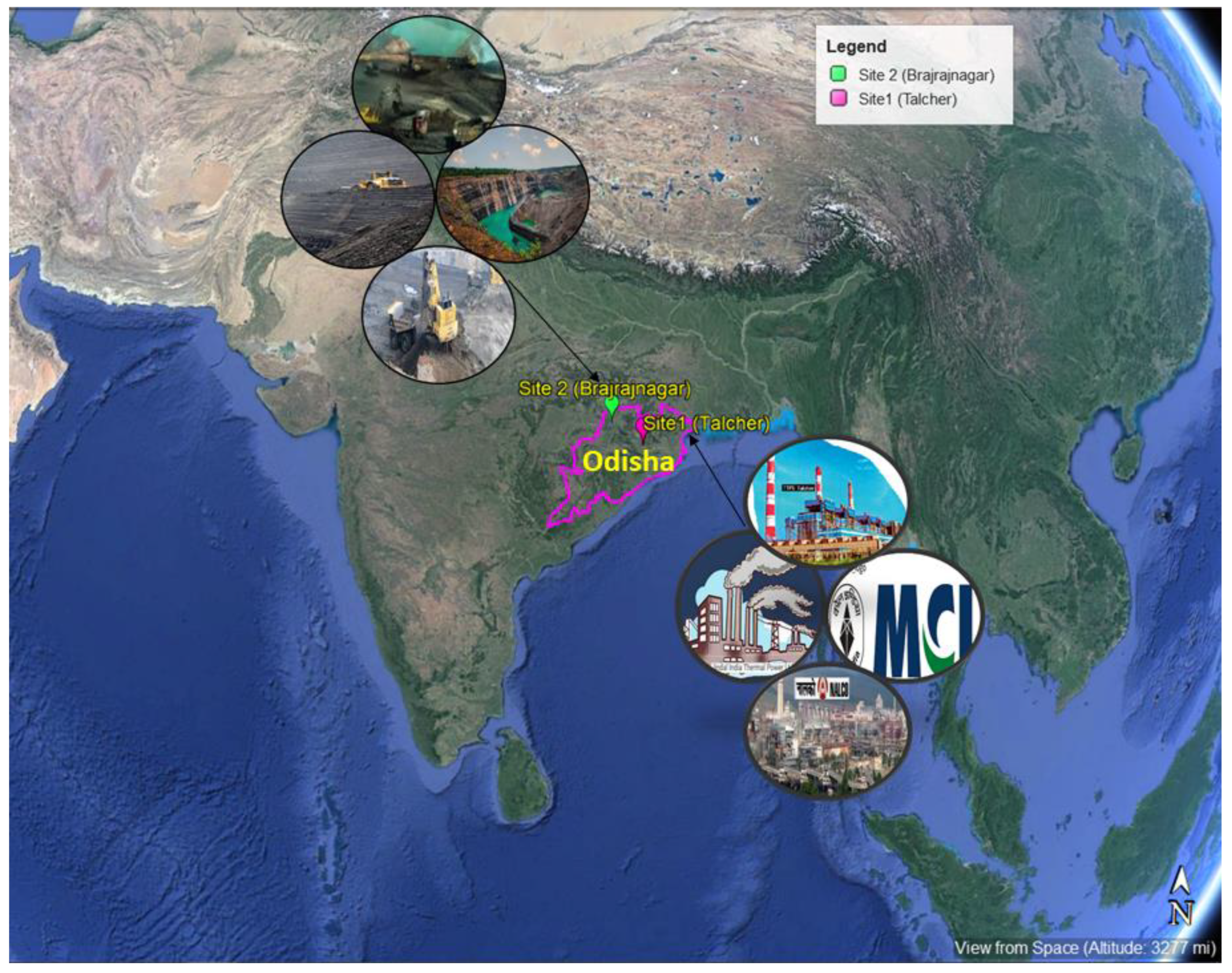
2.1. Study Area
2.2. Data Resources
2.3. Health Risk, Mortality, and Economic Loss
3. Results
3.1. Spatiotemporal Variation of Air Pollutants
3.1.1. Particulate Matter
3.1.2. CO
3.1.3. SO2
3.1.4. NO2 and NOX
3.1.5. O3
3.2. Air Pollutants and Meteorological Parameters
3.3. Diurnal Variation of Pollutants
3.3.1. Diurnal Variation of Particulate Matter
3.3.2. Diurnal Variation of NO2, NOx, and O3
3.3.3. Diurnal Variation of CO
3.3.4. Diurnal Variation of SO2
3.4. Comparative Fundamental Statistics of Pollutants
4. Health Risk, Premature Death, and Economic Cost Associated with Pollutants
5. Discussion
6. Conclusions
Supplementary Materials
Author Contributions
Funding
Institutional Review Board Statement
Informed Consent Statement
Data Availability Statement
Acknowledgments
Conflicts of Interest
References
- Li, X.; Jin, L.; Kan, H. Air Pollution: A Global Problem Needs Local Fixes; Springer Nature: Cham, Switzerland, 2019; pp. 437–439. [Google Scholar]
- Caselles, J.; Colliga, C.; Zornoza, P. Evaluation of trace element pollution from vehicle emissions in petunia plants. Water Air Soil Pollut. 2002, 136, 1–9. [Google Scholar] [CrossRef]
- Curtis, L.; William, R.; Patricia, S.W.; Ervin, F.; Yaqin, P. Adverse health effects of outdoor air pollutants. Environ. Int. 2006, 32, 815–830. [Google Scholar] [CrossRef]
- World Health Organization. Air Pollution and Child Health: Prescribing Clean Air: Summary (No. WHO/CED/PHE/18.01); World Health Organization: Geneva, Switzerland, 2018. [Google Scholar]
- Kumar, P.; Pratap, V.; Kumar, A.; Choudhary, A.; Prasad, R.; Shukla, A.; Singh, R.P.; Singh, A.K. Assessment of atmospheric aerosols over Varanasi: Physical, optical and chemical properties and meteorological implications. J. Atmos. Sol. Terr. Phys. 2020, 209, 105424. [Google Scholar] [CrossRef]
- Kumar, P.; Kapur, S.; Choudhary, A.; Singh, A.K. Spatiotemporal variability of optical properties of aerosols over the Indo-Gangetic Plain during 2011–2015. Indian J. Phys. 2022, 96, 329–341. [Google Scholar] [CrossRef]
- Gurjar, B.R.; Ravindra, K.; Nagpure, A.S. Air pollution trends over Indian megacities and their local-to-global implications. Atmos. Environ. 2016, 142, 475–495. [Google Scholar] [CrossRef]
- Choudhary, A.; Gokhale, S. Urban real-world driving traffic emissions during interruption and congestion. Transp. Res. D Trans. Environ. 2016, 43, 59–70. [Google Scholar] [CrossRef]
- Schembari, C.; Cavalli, F.; Cuccia, E.; Hjorth, J.; Calzolai, G.; Pérez, N.; Pey, J.; Prati, P.; Raes, F. Impact of a European directive on ship emissions on air quality in Mediterranean harbours. Atmos. Environ. 2012, 61, 661–669. [Google Scholar] [CrossRef]
- Choudhary, A.; Gokhale, S. Evaluation of emission reduction benefits of traffic flow management and technology upgrade in a congested urban traffic corridor. Clean Technol. Environ. Pol. 2019, 21, 257–273. [Google Scholar] [CrossRef]
- Shah, K.; Amin, N.; Ahmad, I.; Shah, S.; Hussain, K. Dust particles induce stress, reduce various photosynthetic pigments and their derivatives in Ficus benjamina: A landscape plant. Int. J. Agric. Biol. 2017, 19, 1469–1474. [Google Scholar]
- Strak, M.; Janssen, N.A.; Gosens, I.; Cassee, F.R.; Lebret, E.; Godri, K.J.; Mudway, I.S.; Kelly, F.J.; Harrison, R.M.; Brunekreef, B.; et al. Airborne particulate matter and acute lung inflammation: Strak et al. respond. Environ. Health Perspect. 2013, 121, a11–a12. [Google Scholar] [CrossRef] [Green Version]
- Atkinson, R.W.; Cohen, A.; Mehta, S.; Anderson, H.R. Systematic review and meta-analysis of epidemiological time-series studies on outdoor air pollution and health in Asia. Air Qual. Atmos. Health 2012, 5, 383–391. [Google Scholar] [CrossRef]
- Wong, C.M.; Vichit-Vadakan, N.; Kan, H.; Qian, Z. Public Health and Air Pollution in Asia (PAPA): A multicity study of short-term effects of air pollution on mortality. Environ. Health Perspect. 2008, 116, 1195–1202. [Google Scholar] [CrossRef] [Green Version]
- Shang, Y.; Sun, Z.; Cao, J.; Wang, X.; Zhong, L.; Bi, X.; Li, H.; Liu, W.; Zhu, T.; Huang, W. Systematic review of Chinese studies of short-term exposure to air pollution and daily mortality. Environ Int. 2013, 54, 100–111. [Google Scholar] [CrossRef]
- Venter, Z.S.; Aunan, K.; Chowdhury, S.; Lelieveld, J. COVID-19 lockdowns cause global air pollution declines. Proc. Natl. Acad. Sci. USA 2020, 117, 18984–18990. [Google Scholar] [CrossRef]
- Saadat, S.; Rawtani, D.; Hussain, C.M. Environmental perspective of COVID-19. Sci. Total Environ. 2020, 728, 138870. [Google Scholar] [CrossRef]
- Sharma, S.; Zhang, M.; Gao, J.; Zhang, H.; Kota, S.H. Effect of restricted emissions during COVID-19 on air quality in India. Sci. Total Environ. 2020, 728, 138878. [Google Scholar] [CrossRef] [PubMed]
- Kumar, P.; Hama, S.; Omidvarborna, H.; Sharma, A.; Sahani, J.; Abhijith, K.V.; Debele, S.E.; Zavala-Reyes, J.C.; Barwise, Y.; Tiwari, A. Temporary reduction in fine particulate matter due to ‘anthropogenic emissions switch-off’ during COVID-19 lockdown in Indian cities. Sustain. Cities Soc. 2020, 62, 102382. [Google Scholar] [CrossRef] [PubMed]
- Das, L.; Patri, M. Impact of Environmental Pollution on Respiratory System of Human and Animals in Angul and Talcher Industrial Areas, Odisha, India: A Case Study. Int. J. Zoo. Animal Biol. 2019, 2, 000162. [Google Scholar]
- Hota, P.; Behera, B. Coal mining in Odisha: An analysis of impacts on agricultural production and human health. Extr. Ind. Soc. 2015, 2, 683–693. [Google Scholar] [CrossRef]
- Cropper, M.; Gamkhar, S.; Malik, K.; Limonov, A.; Partridge, I. The health effects of coal electricity generation in India. Resour. Future Discuss. Pap. 2012, 12–25. [Google Scholar] [CrossRef]
- Mishra, N.; Das, N. Coal Mining and Local Environment: A Study in Talcher Coalfield of India. Air Soil Water Res. 2017, 10, 1–17. [Google Scholar] [CrossRef]
- MSME. Brief Industrial Profile of Angul District; MSME: New Delhi, India, 2020. [Google Scholar]
- Annual Report, 2021a. Annual Ruteen Environmental Monitoring Report 2019–2020, Talcher Coalfield. Available online: https://www.mahanadicoal.in/Environment/Environmental_Monitoring_Report.php (accessed on 15 June 2022).
- Annual Report, 2021b. Annual Ruteen Environmental Monitoring Report 2019–2020, IB-Valley Coalfield. Available online: https://www.mahanadicoal.in/Environment/Environmental_Monitoring_Report.php (accessed on 15 June 2022).
- CPCB. Air Quality Comparison Report; Central Pollution Control Board: New Delhi, India, 2020. [Google Scholar]
- Hu, J.; Ying, Q.; Wang, Y.; Zhang, H. Characterizing multi-pollutant air pollution in China: Comparison of three air quality indices. Environ. Int. 2015, 84, 17–25. [Google Scholar] [CrossRef] [PubMed]
- Ghude, S.D.; Chate, D.M.; Jena, C.; Beig, G.; Kumar, R.; Barth, M.C.; Pfister, G.G.; Fadnavis, S.; Pithani, P. Premature mortality in India due to PM2.5 and ozone exposure. Geophys. Res. Lett. 2016, 43, 4650–4658. [Google Scholar] [CrossRef] [Green Version]
- Shanmugam, K. The value of life: Estimates from Indian Labour Market. Indian Econ. J. 1996, 44, 105–114. [Google Scholar] [CrossRef]
- Cropper, M.; Simon, N.B.; Alberini, A.; Arora, S. Valuing Mortality Reductions in India: A Study of Compensating-Wage Differentials; World Bank Group: Washington, DC, USA, 1999. [Google Scholar] [CrossRef]
- Bherwani, H.; Nair, M.; Musugu, K.; Gautam, S.; Gupta, A.; Kapley, A.; Kumar, R. Valuation of air pollution externalities: Comparative assessment of economic damage and emission reduction under COVID-19 lockdown. Air Qual. Atmos. Health 2020, 13, 683–694. [Google Scholar] [CrossRef] [PubMed]
- Sathe, Y.; Gupta, P.; Bawase, M.; Lamsal, L.; Patadia, F.; Thipse, S. Surface and satellite observations of air pollution in India during COVID-19 lockdown: Implication to air quality. Sustain. Cities Soc. 2021, 66, 102688. [Google Scholar] [CrossRef] [PubMed]
- Parida, B.R.; Bar, S.; Roberts, G.; Mandal, S.P.; Pandey, A.C.; Kumar, M.; Dash, J. Improvement in air quality and its impact on land surface temperature in major urban areas across India during the first lockdown of the pandemic. Environ. Res. 2021, 199, 111280. [Google Scholar] [CrossRef]
- Thomas, J.; Jainet, P.J.; Sudheer, K.P. Ambient air quality of a less industrialized region of India (Kerala) during the COVID-19 lockdown. Anthropocene 2020, 32, 100270. [Google Scholar] [CrossRef]
- Resmi, C.T.; Nishanth, T.; Satheesh Kumar, M.K.; Manoj, M.G.; Balachandramohan, M.; Valsaraj, K.T. Air quality improvement during triple-lockdown in the coastal city of Kannur, Kerala to combat Covid-19 transmission. Peer J. 2020, 8, e9642. [Google Scholar] [CrossRef]
- Sahu, S.K.; Beig, G.; Parkhi, N. Critical emissions from the largest on-road transport network in South Asia. Aerosol Air Qual. Res. 2014, 14, 135–144. [Google Scholar] [CrossRef] [Green Version]
- Singh, V.; Biswal, A.; Kesarkar, A.P.; Mor, S.; Ravindra, K. High resolution vehicular PM10 emissions over megacity Delhi: Relative contributions of exhaust and non-exhaust sources. Sci. Total Environ. 2020, 699, 134273. [Google Scholar] [CrossRef] [PubMed]
- Lu, Z.; Streets, D.G. Increase in NOx emissions from Indian thermal power plants during 1996–2010: Unit-based inventories and multi satellite observations. Environ. Sci. Technol. 2012, 46, 7463–7470. [Google Scholar] [CrossRef] [PubMed]
- Ghude, S.D.; Fadnavis, S.; Beig, G.; Polade, S.D.; Van Der A, R.J. Detection of surface emission hot spots, trends, and seasonal cycle from satellite-retrieved NO2 over India. J. Geophys. Res. Atmos. 2008, 113, D20. [Google Scholar] [CrossRef] [Green Version]
- Garg, A.; Shukla, P.R.; Bhattacharya, S.; Dadhwal, V.K. Sub-region (district) and sector level SO2 and NOx emissions for India: Assessment of inventories and mitigation flexibility. Atmos. Environ. 2001, 35, 703–713. [Google Scholar] [CrossRef]
- Mahato, S.; Ghosh, K.G. Short-term exposure to ambient air quality of the most polluted Indian cities due to lockdown amid SARS-CoV-2. Environ. Res. 2020, 188, 109835. [Google Scholar] [CrossRef]
- Mallik, C.; Mahapatra, P.S.; Kumar, P.; Panda, S.; Boopathy, R.; Das, T.; Lal, S. Influence of regional emissions on SO2 concentrations over Bhubaneswar, a capital city in eastern India downwind of the Indian SO2 hotspots. Atmos. Environ. 2019, 209, 220–232. [Google Scholar] [CrossRef]
- Hendryx, M.; Zullig, K.J.; Luo, J. Impacts of coal use on health. Annu. Rev. Public Health 2020, 41, 397–415. [Google Scholar] [CrossRef] [PubMed] [Green Version]
- Mishra, S.K. Putting value to human health in coal mining region of India. J. Health Manag. 2015, 17, 339–355. [Google Scholar] [CrossRef]
- Guttikunda, S.K.; Jawahar, P. Evaluation of particulate pollution and health impacts from planned expansion of coal-fired thermal power plants in India using WRF-CAMx modeling system. Aerosol Air Qual. Res. 2018, 18, 3187–3202. [Google Scholar] [CrossRef]
- Cropper, M.; Cui, R.; Guttikunda, S.; Hultman, N.; Jawahar, P.; Park, Y.; Yao, X.; Song, X.P. The mortality impacts of current and planned coal-fired power plants in India. Proc. Natl. Acad. Sci. USA 2021, 118, e2017936118. [Google Scholar] [CrossRef]
- Lal, S.; Naja, M.; Subbaraya, B.H. Seasonal variations in surface ozone and its precursors over an urban site in India. Atmos. Environ. 2000, 34, 2713–2724. [Google Scholar] [CrossRef]
- Reddy, B.S.; Kumar, K.R.; Balakrishnaiah, G.; Gopal, K.R.; Reddy, R.R.; Sivakumar, V.; Lingaswamy, A.P.; Arafath, S.M.; Umadevi, K.; Kumari, S.P.; et al. Analysis of diurnal and seasonal behavior of surface ozone and its precursors (NOx) at a semi-arid rural site in southern India. Aerosol Air Qual. Res. 2012, 12, 1081–1094. [Google Scholar] [CrossRef] [Green Version]
- Kumar, V.; Sinha, V. Season-wise analyses of VOCs, hydroxyl radicals and ozone formation chemistry over north-west India reveal isoprene and acetaldehyde as the most potent ozone precursors throughout the year. Chemosphere 2021, 283, 131184. [Google Scholar] [CrossRef] [PubMed]
- Ampah, J.D.; Jin, C.; Agyekum, E.B.; Afrane, S.; Geng, Z.; Adun, H.; Yusuf, A.A.; Liu, H.; Bamisile, O. Performance analysis and socio-enviro-economic feasibility study of a new hybrid energy system-based decarbonization approach for coal mine sites. Sci. Total Environ. 2022, 854, 158820. [Google Scholar] [CrossRef] [PubMed]


| Year | PM2.5 | PM10 | CO | SO2 | NO2 | NOx | O3 |
|---|---|---|---|---|---|---|---|
| (µg/m3) | (ppm) | (ppb) | |||||
| Site #1 | |||||||
| 2019 | 38.80 ± 13.54 | 159.36 ± 53.28 | 1.23 ± 0.29 | 25.98 ± 2.96 | 13.06 ± 3.48 | 25.33 ± 4.49 | 5.41 ± 1.83 |
| LD2020 | 41.66 ± 22.11 | 165.15 ± 92.33 | 1.88 ± 0.31 | 19.88 ± 6.69 | 12.76 ± 9.45 | 24.94 ± 18.68 | 44.87 ± 9.29 |
| LD2021 | 37.92 ± 10.12 | 162.14 ± 55.89 | 1.73 ± 0.27 | 13.84 ± 4.96 | 28.22 ± 5.78 | 49.00 ± 7.78 | 25.33 ± 5.04 |
| Site #2 | |||||||
| 2019 | 69.88 ± 31.51 | 152.88 ± 54.76 | 2.65 ± 0.50 | 7.51 ± 1.26 | 19.66 ± 4.25 | 29.85 ± 9.56 | 10.96 ± 3.61 |
| LD2020 | 78.35 ± 30.61 | 171.94 ± 64.57 | 1.11 ± 0.28 | 4.92 ± 1.05 | 3.35 ± 1.64 | 20.42 ± 5.10 | 54.91 ± 15.08 |
| LD2021 | 61.09 ± 11.56 | 143.29 ± 28.32 | 2.26 ± 0.13 | 4.83 ± 0.49 | 22.02 ± 10.07 | 37.55 ± 9.66 | 21.79 ± 16.69 |
| Sites | Year | Annual/ Lockdown | Pollutant-Wise Death Attribution/100,000 | Total Attributed Deaths/100,000 | EC (USD in Million) | ||||
|---|---|---|---|---|---|---|---|---|---|
| PM2.5 | PM10 | NO2 | SO2 | O3 | |||||
| Site #1 | 2019 | Annual Pre-lockdown | 47 | 84 | 26 | 24 | 6 | 187 (54%) | 109 |
| 7 | 10 | 5 | 4 | 3 | 30 (52%) | 17.6 | |||
| 2020 | annual | 61 | 85 | 38 | 33 | 15 | 233 (63%) | 137 | |
| LD2020 | 7 | 11 | 9 | 6 | 4 | 37 (52%) | 22 | ||
| 2021 | annual | 62 | 113 | 32 | 17 | 8 | 232 (62%) | 136 | |
| LD2021 | 7 | 11 | 9 | 9 | 1 | 37 (60%) | 22 | ||
| Site #2 | 2019 | annual | 24 | 54 | 21 | 20 | 11 | 130 (58%) | 76 |
| Pre-lockdown | 5 | 10 | 2 | 2 | 0 | 19 (50%) | 11 | ||
| 2020 | annual | 31 | 56 | 27 | 25 | 8 | 147 (61%) | 86 | |
| LD2020 | 5 | 9 | 3 | 4 | 1 | 23 (58%) | 14 | ||
| 2021 | annual | 29 | 63 | 25 | 25 | 8 | 151 (62%) | 89 | |
| LD2021 | 5 | 10 | 4 | 4 | 1 | 24 (60%) | 14 | ||
Publisher’s Note: MDPI stays neutral with regard to jurisdictional claims in published maps and institutional affiliations. |
© 2022 by the authors. Licensee MDPI, Basel, Switzerland. This article is an open access article distributed under the terms and conditions of the Creative Commons Attribution (CC BY) license (https://creativecommons.org/licenses/by/4.0/).
Share and Cite
Choudhary, A.; Kumar, P.; Sahu, S.K.; Pradhan, C.; Joshi, P.K.; Singh, S.K.; Kumar, P.; Mezoue, C.A.; Singh, A.K.; Tyagi, B. Health Risk Appraisal Associated with Air Quality over Coal-Fired Thermal Power Plants and Coalmine Complex Belts of Urban–Rural Agglomeration in the Eastern Coastal State of Odisha, India. Atmosphere 2022, 13, 2064. https://doi.org/10.3390/atmos13122064
Choudhary A, Kumar P, Sahu SK, Pradhan C, Joshi PK, Singh SK, Kumar P, Mezoue CA, Singh AK, Tyagi B. Health Risk Appraisal Associated with Air Quality over Coal-Fired Thermal Power Plants and Coalmine Complex Belts of Urban–Rural Agglomeration in the Eastern Coastal State of Odisha, India. Atmosphere. 2022; 13(12):2064. https://doi.org/10.3390/atmos13122064
Chicago/Turabian StyleChoudhary, Arti, Pradeep Kumar, Saroj Kumar Sahu, Chinmay Pradhan, Pawan Kumar Joshi, Sudhir Kumar Singh, Pankaj Kumar, Cyrille A. Mezoue, Abhay Kumar Singh, and Bhishma Tyagi. 2022. "Health Risk Appraisal Associated with Air Quality over Coal-Fired Thermal Power Plants and Coalmine Complex Belts of Urban–Rural Agglomeration in the Eastern Coastal State of Odisha, India" Atmosphere 13, no. 12: 2064. https://doi.org/10.3390/atmos13122064
APA StyleChoudhary, A., Kumar, P., Sahu, S. K., Pradhan, C., Joshi, P. K., Singh, S. K., Kumar, P., Mezoue, C. A., Singh, A. K., & Tyagi, B. (2022). Health Risk Appraisal Associated with Air Quality over Coal-Fired Thermal Power Plants and Coalmine Complex Belts of Urban–Rural Agglomeration in the Eastern Coastal State of Odisha, India. Atmosphere, 13(12), 2064. https://doi.org/10.3390/atmos13122064