Influence of Planetary Boundary Layer (PBL) Parameterizations in the Weather Research and Forecasting (WRF) Model on the Retrieval of Surface Meteorological Variables over the Kenyan Highlands

Abstract

Regional climate models (RCMs) are crucial for climate studies and may be an alternative source of meteorological data in data-scarce regions. However, the effectiveness of the numerical weather prediction (NWP) models applied in RCMs is hampered by the parameterization of unresolved physical processes in the model. A major source of uncertainties in NWP models is the parameterization of the planetary boundary layer (PBL). This study evaluates the influence of seven PBL parameterization schemes in the Weather Research and Forecasting (WRF) model on the retrieval of four meteorological variables over the Kenyan highlands. The seven PBL schemes consist of four local schemes: the Mellor-Yamada-Janjic (MYJ), Mellor-Yamada-Nakanishi-Niino (MYNN), Bougeault-Lacarrere (BouLac), quasinormal scale elimination (QNSE), and three nonlocal schemes: asymmetrical convective model version 2 (ACM2), Shin and Hong (SHIN) and Yonsei University (YSU). The forcing data for the WRF model was obtained from the fifth generation of the European ReAnalysis (ERA5) dataset. The results were validated against observational data from the Trans-African Hydro-Meteorological Observatory (TAHMO). WRF was found to simulate surface meteorological variables with spatial details coherent with the complex topography within the Kenyan highlands, irrespective of the PBL scheme. A comparison between 2-meter temperature (T2) derived from the YSU scheme and T2 from the land component of ERA5 (ERA5-Land) indicates that surface meteorological variables derived from WRF are better suited for applications over the Kenyan highlands. The choice of the PBL scheme was found to primarily influence the simulation of the 10-meter wind speed (WS10) and rainfall as opposed to T2 and the 2-meter relative humidity (RH2). The insensitivity of the 2-meter variables to the choice of the PBL scheme is attributed to the influence of the surface layer parameterization near the surface. Results from the rainfall simulation indicate that the YSU scheme provides a more realistic depiction of PBL dynamics within the study area. Hence, the YSU scheme is best suited for simulating surface meteorological variables over the Kenyan highlands.

1. Introduction

Regional climate models (RCMs) are increasingly being adopted in studies and applications at the regional and local scale to provide quality spatial-temporally refined weather and climate-related variables [1]. The RCM concept, also known as dynamical downscaling, applies high-resolution numerical weather prediction (NWP) models over regional model domains to resolve the sub-grid variability in the climate fields derived from general circulation models (GCMs). The climate fields from the GCM, which describe the global atmospheric circulation response to large-scale forcings related to the Earth’s differential heating, are used as the initial and lateral boundary conditions in RCMs. On the other hand, a better representation of the physics in the NWP model is used to describe the processes’ influence at the local scale related to orography, inland water bodies, vegetation, and land use [2]. Cognizant to the importance of local-scale processes, especially for land applications, GCM derived datasets with a relatively high resolution, e.g., the land component of the fifth generation of European ReAnalysis (ERA5) dataset [3] referred to as ERA5-land, have been developed. The ERA5-land dataset has the highest spatial resolution (9 km) currently available of any dataset of its kind. However, the dataset is still too coarse to effectively capture the local-scale processes, especially in regions characterized by complex terrain, emphasizing the need for RCMs.

Generally, an RCM utilizes a cascade of nested model domains of increasing spatial resolutions in the inner model domains at predefined nesting ratios, allowing for a physically-based interpolation of the GCM-derived climate fields to the regional and local scales. A major challenge in the application of RCMs is that they are not readily transferable due to the sensitivity of models to the initial and lateral boundary conditions, differences in the physical processes characteristic to a region, and the choice of physics schemes [1,3,4,5]. The representation of the unresolved physical processes, popularly referred to as parameterization, has been cited as a major source of uncertainties in NWP models [6]. As such, scores of studies have been carried out to analyze the effects of various parameterizations on the prediction skill of NWP models, e.g., cumulus parameterization [7,8,9], cloud microphysics [10,11,12], planetary boundary layer (PBL) parameterization [13,14,15], among other studies. The forecast skill of NWP models has been shown to be highly sensitive to PBL parameterizations [16,17]. For instance, a study by Li and Pu [13] found that the parameterization of the PBL was as influential to the development of hurricane intensity and associated precipitation in a similar manner to the parameterization of cloud microphysics, further emphasizing the importance of PBL parameterization in NWP models.

The PBL is defined as that portion of the troposphere that responds directly to forcings emanating from the Earth’s surface at timescales of one hour or less [18]. The PBL layer is characterized by a strong vertical mixing and a marked diurnal variation in depth. The PBL plays an important role in the development of weather phenomena due to the exchange of heat and momentum fluxes between the land surface and the atmosphere through turbulence transport. However, the complex, chaotic nature of turbulent flow due to eddies of disproportionate sizes and time lengths within the PBL limits the explicit solution of the governing equations of atmospheric flow. Thus, PBL parameterizations suffice as efficient approximate solutions for turbulence in the atmospheric flow. PBL parameterizations are used to describe the background (time-averaged) atmospheric state and the perturbations (deviations) from the mean state associated with turbulent motions within the PBL based on the Reynolds averaging technique [6]. PBL parameterization schemes are classified into first-order closure or higher-order turbulent kinetic energy (TKE) closure schemes. First-order closure schemes do not require additional prognostic equations to describe the effects of turbulence on the mean flow variables. In addition, first-order closure schemes allow for the exchange of fluxes between all layers in the PBL through large convective eddies and are thus also referred to as nonlocal closure schemes. On the other hand, higher-order TKE closure schemes include an additional prognostic equation for the TKE. TKE closure schemes are also known as local closure schemes since they only allow for the exchange of fluxes between adjacent model layers. Generally, local order closure schemes are suited for the simulation of stable boundary layers, whereas nonlocal schemes are better at simulating unstable boundary layers characterized by strong convection [6,15]. However, as reported in García-Díez et al. [3], PBL schemes are highly sensitive to seasonality, forecast length, and geographic location and thus may not necessarily produce consistent results across a spectrum of atmospheric conditions.

Several studies aimed at evaluating the performance of PBL parameterization schemes across regions and under varying weather phenomena have been carried out. Among them is the study by Shin and Hong [15], who compared the performance of five PBL parameterization schemes available in the Weather Research and Forecasting (WRF) model under stable and unstable atmospheric conditions in Kansas, USA. They found that PBL parameterization schemes based on local mixing approaches generally performed better under stable conditions than those based on a nonlocal mixing approach. The opposite was found to be true for unstable conditions. Cohen et al. [18], analyzed the ability of PBL schemes in the WRF model to simulate two tornado events in the southeastern USA. They reported a better representation of the lapse rates within the first three kilometers using nonlocal schemes as opposed to the local schemes. In addition, they observed that the nonlocal schemes were less biased in the retrieval of temperature fields, which they attributed to a better representation of entrainment processes in nonlocal schemes. Similar findings have been reported in Avolio et al. [14], in southern Italy, during an experimental campaign; Banks et al. [19], over Athens in Greece; Hazra and Pattnaik [20], over Odisha state in India; and Boadh et al. [21], over a tropical station in India. Contrastingly, in a study by Chaouch et al. [22], local schemes were found to represent PBL variables and structure relatively well compared to nonlocal schemes under dry fog conditions in the United Arab Emirates. Better performance with local parameterization schemes has also been reported in Ooi et al. [23], over Kuala Lumpur, Malaysia; Tyagi et al. [24], in Southern Italy; Madala et al. [25], in a region in India; Gbode et al. [26], in a monsoon regime over West Africa; and in de Lange et al. [27], in the Highveld region of South Africa. However, as reported in Hazra and Pattnaik [20] and Yang et al. [28], the skill of a PBL scheme varies widely depending on the target variable. The findings by García-Díez et al. [3], Hazra and Pattnaik [20], Yang et al. [28], and Li and Pu [13], among others, emphasize the need to evaluate the impacts of PBL parameterization schemes on RCMs.

The Kenyan highlands rank among the most vulnerable regions to climate change and variability globally [29]. According to projections presented in Gebrechorkos et al. [30], the region is expected to witness a significant rise in extreme climate-related events, such as floods and droughts. On the other hand, the region is among the most meteorologically poorly gauged regions in the world [31]. As such, RCM provides an alternative source of meteorological data to support the monitoring and sustainable use of natural resources and the implementation of climate adaptation and mitigation strategies in the region. Although several studies related to RCM have been conducted in this region [7,32,33], most of them have focused on the sensitivity of RCMs to the parameterization of cumulus and cloud microphysics schemes in simulating precipitation. This study evaluates how the various PBL schemes in the Weather Research and Forecasting (WRF) model influence the retrieval of surface meteorological variables over the Kenyan highlands.

2. Materials and Methods

2.1. Model Description

Since its release in 2000, the Weather Research and Forecasting (WRF) model has become one of the most widely used atmospheric models [34]. WRF is a mesoscale NWP model designed for atmospheric research and operational weather forecasting and is suitable for applications ranging in scale from hundreds of meters to several kilometers. WRF simulations can either be real cases (based on observational or analysis datasets) or idealized simulation experiments. The WRF model simulates the atmospheric state and its evolution, and amongst its outputs are various columnar and surface meteorological variables. Consequently, the WRF modeling framework has been applied in multiple applications ranging from but not limited to; air pollution studies, hydrology, hurricanes, regional climate studies, urban heat island, and others [34,35].

WRF comprises a suite of physical parameterizations and dynamics representing interactions between the land surface and the atmosphere. Different physical parameterizations are used in WRF to describe the PBL, radiation budget, cumulus processes, cloud microphysics, the surface layer, and the land surface. The model architecture allows for portability, data assimilation, system extensibility, and parallel computing. WRF consists of two dynamic solvers (cores), namely the Nonhydrostatic Mesoscale Model (NMM) core developed at the National Centers for Environmental Prediction (NCEP) and the Advanced Research WRF (ARW) core mainly developed and maintained by the National Center for Atmospheric Research (NCAR) with broad support from the model’s community user base. The NMM core is essentially a fully compressible hydrostatic model modified by Janjic [36] through an add-on module that can be turned on to account for non-hydrostatic motions. On the other hand, the ARW core [37] is a fully compressible Euler-based non-hydrostatic model, which includes a run-time hydrostatic option. The ARW core uses a terrain-following vertical grid stretching permitting dry hydrostatic-pressure vertical coordinates with an invariant pressure surface model top. The horizontal grid is based on the Arakawa C-grid staggering and supports four different map projections for real data simulations. Being a non-hydrostatic model, the ARW core is more suitable for representing sub-grid scale processes than the NMM core. In addition, thanks to contributions from its immense community user base, a wider range of physical parameterization options are available in the ARW core than in the NMM core. As a result, the ARW core is the most widely used WRF core in RCM studies.

2.2. PBL Parameterization Schemes in WRF

This study utilized the WRF-ARW model version 4.0.3. This version of the model includes twelve PBL parameterization schemes. Seven commonly used schemes were evaluated in this study. Each of these schemes is briefly described in this section.

2.2.1. Asymmetrical Convective Model Version 2

The asymmetrical convective model version 2 (ACM2) scheme [38,39] is a first-order closure scheme. It is a hybrid local, nonlocal closure scheme. In the ACM2 scheme, the upward fluxes from the surface interact with each layer to account for convective plumes emanating from the surface. On the other hand, the downward fluxes only interact between adjacent layers. Eddy diffusion is treated locally for both the upward and downward fluxes. The scheme utilizes only the local mixing for upward and downward mixing in stable or neutral flow regimes. In ACM2, the calculation of the PBL height is based on the bulk Richardson number (Ri_B). It is determined as the height where the Ri_B calculated above the neutral buoyancy level is greater than a critical Ri_B value of 0.25. According to validation results by Pleim [38], the inclusion of both local and nonlocal mixing in the scheme improves the depiction of the profiles of potential temperature and velocity within the PBL layer. However, Coniglio et al. [40] report that the scheme produces PBLs that are too deep in the evening compared to sounding data.

2.2.2. Bougeault-Lacarrere Scheme

The Bougeault-Lacarrere (BouLac) scheme [41] is a 1.5-order local closure scheme based on a prognostic equation for TKE. The second-order moments in the prognostic equation for TKE are parameterized based on an eddy coefficient approximation. The turbulence length scale is parameterized based on the mean TKE of the layer and buoyancy and is specifically designed to capture turbulence induced by gravity waves in complex terrain. The scheme also includes a counter gradient term to account for the effects of large eddies in convective cases. In this scheme, PBL height is calculated as the height where TKE falls below a prescribed threshold. Shin and Hong [15] report that the scheme shows a better ability to represent the PBL under high static stability conditions than nonlocal schemes. However, just like with most of the other local schemes, the scheme does not efficiently capture the effects of large eddies, leading to undermixing in convective PBLs [18].

2.2.3. Mellor-Yamada-Janjic Scheme

The Mellor-Yamada-Janjic (MYJ) scheme [42] is a 1.5-order local closure scheme based on a prognostic equation for the TKE. In this scheme, nonlocal transport associated with large eddies is accounted for by adding a counter gradient term in the heat and momentum transport equation. The scheme also includes a TKE diffusion outside the mixed layer, which, combined with the counter gradient transport, improves the representation of the entrainment at the top of the PBL. The PBL height is designated as the height at which the TKE falls below a TKE threshold of 0.2 m² s⁻². One of the limitations of the MYJ scheme is the underdevelopment of PBL during convective regimes resulting in a shallow cold and moist PBL [40].

2.2.4. Mellor-Yamada-Nakanishi-Niino Scheme

The Mellor-Yamada-Nakanishi-Niino Level 2.5 (MYNN) scheme [43,44], similar to the MYJ, is a 1.5-order local closure scheme based on a prognostic equation for TKE. Unlike the MYJ scheme, which uses observations to derive expressions of stability and mixing length, the MYNN scheme uses results from large eddy simulations (LES) to derive these expressions. The revisions to the expressions of the mixing length in the MYNN scheme make it suitable for applications over a wider range of static stability regimes than the MYJ scheme [18]. The MYNN scheme has also been found to better represent deep convective springtime PBL compared to nonlocal schemes [40]. However, just like the other local closure schemes, the MYNN scheme does not fully account for deeper vertical mixing induced by large eddies [18].

2.2.5. Quasinormal Scale Elimination Scheme

The quasinormal scale elimination (QNSE) scheme [45] is a 1.5-order local closure scheme. It is a spectral model designed for turbulent flows characterized by stable stratification. The scheme employs a quasi-Gaussian mapping of the velocity and temperature fields to account for wave phenomena in stable boundary layers. A stratification scale-dependent elimination algorithm explicitly accounts for the combined effect of turbulence and internal waves. As stratification increases, energy is accumulated in the horizontal flow components at the expense of the energy for the vertical flow components. The scheme calculates the PBL height as the height at which the TKE profile decreases to a value of 0.01 m² s⁻². The scheme has provided a realistic depiction of potential temperature and kinematic profiles under stable conditions [18]. However, under unstable conditions, the scheme produces PBLs that are too shallow, cool, and moist [40].

2.2.6. Shin and Hong Scheme

The Shin and Hong (SHIN) scheme [46] is a first-order nonlocal closure scheme designed to capture the effect of grid size dependency on turbulent transport in convective boundary layers. Effects of large eddies are represented through a nonlocal transport profile fitted to LES simulation outputs. On the other hand, local transport is derived using an eddy diffusivity-based transport equation. A grid-size dependent function formulated by Shin and Hong [47] is used to scale local and nonlocal transport within the boundary layer. According to Shin and Hong [46], the scheme performs better under convective boundary layers than the conventional nonlocal schemes.

2.2.7. Yonsei University Scheme

The Yonsei University (YSU) scheme [48] is a first-order nonlocal closure scheme. It utilizes a turbulence diffusion equation to derive prognostic flux variables within the mixed layer based on an eddy diffusivity coefficient and a counter gradient correction term. The counter gradient correction term accounts for the contribution of the large-scale eddies to the total flux. In the YSU scheme, entrainment is explicitly parameterized through an additional term in the turbulence diffusion equation. The scheme calculates the PBL height by considering Ri_b values calculated from the surface. For unstable cases, a critical Ri_B value of 0.25 is adopted, while the value is set to zero for stable cases. Although the YSU scheme is more effective at representing deep vertical mixing in convective PBLs than most of the other schemes, it has been found to simulate springtime convective PBLs that are too deep, resulting in too dry of air near the surface [18].

2.3. Study Area and Experimental Design

The study area primarily covers the Kenyan highlands and corresponds to the innermost (D03) WRF model domain, as shown in Figure 1. The region experiences two rainy seasons, with the ‘long rains’ season occurring in March, April, and May (MAM). On the other hand, the ‘short rains’ season occurs in October, November, and December (OND). In between the two rainy seasons, the region is generally dry. The seasonality in this region is mainly attributed to the intertropical convergence zone (ITCZ) and its associated monsoon winds [7,33]. The monsoon winds influence the seasonal variation in moisture within the region. On the other hand, the highly variable topography in the region modulates the available moisture at the local scale resulting in high spatial variability in the distribution of rainfall and other meteorological variables. Between November and March, a northeasterly/easterly, Indian monsoon-induced flow dominates the region and gradually shifts into easterly flow between March and May [49]. The period between May and October is dominated by southeasterly monsoon winds. The dry seasons generally coincide with months (July-September, and December-February) when the monsoons are at their peak. The period between December and February is generally hot and dry. On the other hand, the period between June and September is mostly cool and dry. During the rainy seasons, most of the low-lying areas are generally hot and humid, whereas higher elevation areas experience cool and humid weather conditions.

The Kenyan highlands contribute to a majority of the agricultural production in Kenya. Furthermore, they serve as the primary water catchment areas in Kenya and are thus critical to the country’s economy and natural ecosystems.

The experimental setup was configured into three one-way nested domains, as shown in Figure 1. The spatial resolution of each of the domains was set at 9, 3, and 1 km for the first (D01), second (D02), and third (D03) nests, respectively. The corresponding grid configuration for the model nests was set at 180 × 180 (D01), 250 × 250 (D02), and 349 × 349 (D03) grids. The Mercator map projection was adopted for the experimental setup. The 30 arc seconds (approximately 0.92 km) spatial resolution surface geographical dataset provided with the WRF model was adopted to define the topography, soil type, land use, leaf area index, albedo, among other surface geographical variables for the model setup.

The modeling scheme consisted of 40 unequally spaced terrain-following vertical model levels with the model top set at 50 hPa. The initial and boundary conditions were defined using forcing data derived from the fifth generation of European ReAnalysis (ERA5) data at a spatial resolution of 0.25° by 0.25°. Although the ERA5 dataset is available at an hourly time step, the model was forced every 6 hours, conforming to the time step commonly adopted in most studies.

The modeling experiment was set up to simulate surface meteorological variables for four months between January and April 2019. A total of seven different simulation runs, each corresponding to an associated PBL scheme, were performed. The experimental setups varied only in terms of the PBL parameterization schemes and their associated surface layer schemes. Each of the model runs was initialized for 1 January 2019 at 00:00 UTC, which corresponds to 03:00 local time (LT), with the end of each run being 30 April 2019 at 00:00 UTC. The first five days (January 1st to January 5th) were used as model spin-up time and thus, were not included in the evaluation of the model results. The study period was separated into the dry (January and February) and wet (March and April) seasons in the evaluation.

All the PBL schemes, apart from the QNSE and MYJ schemes, utilized the revised MM5 surface layer scheme [50]. The QNSE scheme was coupled to the QNSE surface layer scheme [45], whereas the Eta similarity surface layer scheme [51] was applied in the MYJ scheme. The rest of the physics options utilized in the model setup are summarized in

Table 1. Physics options for the WRF model configuration.

Physics	Parameterization Scheme	Reference
Cloud Microphysics	WRF Single-moment 5-class	Hong, Dudhia and Chen [52]
Shortwave Radiation	Dudhia Shortwave Radiation Scheme	Dudhia [53]
Longwave Radiation	RRTM Longwave Radiation Scheme	Mlawer et al. [54]
Land Surface Model	Unified Noah Land Surface Model	Chen and Dudhia [55]

.

Although a full-year simulation or more would have been ideal for capturing the influence of seasonality on the simulations, the length of the simulations was limited to the available computing resources. The simulations were achieved through the help of a computing grant from the Dutch national supercomputing center (SURFsara). The available grant was enough to simulate a period of four months for each simulation. As such, the period between January and April was chosen since it consists of roughly two dry months (January and February) and two wet months (March and April) for most of the study area. The simulations were carried out on the Cartesius computing cluster at SURFsara.

2.4. Validation

The results of the simulations were validated against surface meteorological data obtained from the Trans-African Hydro-Meteorological Observatory (TAHMO) [31]. The locations of the stations within the study area are shown in Figure 1. In order to ascertain the data quality of TAHMO, a comparison between TAHMO observations and observation data obtained from the Global Surface Summary of the Day (GSOD) was carried out. The comparison was limited to one location where a TAHMO station coincided with a GSOD station. Details and results of the comparison are presented in Appendix A and Figure A1. The variables considered are the air temperature and relative humidity at 2-meter height, wind speed, and precipitation. The temporal resolution of the observations was five minutes and was eighteen seconds for the model, corresponding to the time step for the inner model domain. The temperature, relative humidity, and wind speed fields from the model were averaged to five-minute values to match the temporal resolution of the observations for comparison. On the other hand, the precipitation values for both the model and the observations were aggregated to hourly and daily totals for comparison. Since the surface wind fields from the WRF model are output at the 10-meter height compared to a 2-meter height for the observational dataset, the wind power law (Equation (1)) was applied to the observed wind speed data to interpolate it to the 10-meter height.

$$u_z=u_r {\left(\frac{z}{z_r}\right)}^{\alpha }$$

(1)

where$u_z$ is the wind speed at the target height$z$, $u_r$ is the wind speed at the reference height$z_r$, and α is a stability-dependent coefficient. An α value of 0.143, which is commonly adopted over land and which assumes neutral atmospheric stability, was used in this study.

The statistical metrics used to evaluate the model performance are the correlation coefficient (R) and the root mean squared error (RMSE). In addition, the Equitable Threat Score (ETS), which is a measure of the skill of a model relative to chance, was used to evaluate the ability of the PBL schemes to simulate rainfall. The theoretical basis and formulation of the ETS can be found in Hogan et al. [56].

3. Results

Figure 2 shows a comparison between maps of T2 derived from the YSU scheme (Figure 2a) versus T2 derived from ERA5-Land (Figure 2b). More spatial variations consistent with the variations in elevation in Figure 1b are observed in the contour map for YSU compared to ERA5. Besides, the YSU scheme-derived T2 map shows a broader range of values compared to ERA5.

The statistical performance for the four meteorological variables considered is presented as probability density function (PDF) plots, as shown in Figure 3 and Figure 4. The results for the R (Figure 3) indicate that overall, the performance of the WRF model in the retrieval of T2 and RH2 is less sensitive to the choice of the PBL scheme than the retrieval of WS10 and rainfall. Relatively higher R values with relatively lower variation are observed in the retrieval of T2 and RH2 compared to WS10 and rainfall. Some very low and even negative correlations were observed for WS10 (Figure 3c) and rainfall (Figure 3d) with some of the schemes.

The distribution of the RMSE for each of the four variables is shown in Figure 4. In general, the RMSE obtained with all the schemes in the retrieval of T2 (Figure 4a) ranged between approximately 1.3 to 3.3 degrees Celsius. Apart from the MYNN, QNSE scheme, and to a lesser extent the ACM2 scheme, RMSE values for T2 with the other schemes mostly ranged between approximately 1.3 and 2.5 degrees Celsius. The MYNN scheme produced relatively higher RMSE values in the retrieval of T2 compared to the rest of the schemes, followed by the QNSE and ACM2 schemes. On the other hand, the MYJ scheme appeared to be the best suited for simulating T2, marginally edging out the BouLac scheme. YSU and SHIN, with similar distributions of RMSE values, ranked third in the retrieval of T2. Regarding the retrieval of RH2 (Figure 4b), the MYJ and the QNSE schemes showed a relatively lower range of RMSE values, ranging between approximately 10% and 16%. However, the MYJ scheme showed a marginally better distribution of RH2 RMSE values than the QNSE scheme. The SHIN, YSU, and MYNN schemes rank third, fourth, and fifth, respectively, in the retrieval of RH2, with their RMSE values ranging between approximately 10.5% and 19.5%. In contrast, BouLac, with RMSE values ranging between approximately 11% and 18%, ranked sixth. The ACM2 scheme showed significantly lower performance than the other schemes, with RMSE values ranging between approximately 12.5% and 24.5%. The distribution of the RMSE values obtained in the simulation of WS10 is shown in Figure 4c. The SHIN scheme showed the least RMSE values compared to the rest of the schemes, ranging from 2.5 km/h to approximately 10 km/h. MYNN, BouLac, YSU, and ACM2 showed similar distributions, with RMSE values ranging between approximately 4.5 km/h and 12 km/h. The lowest performance was observed with the QNSE and MYJ schemes, with their RMSE values ranging between approximately 6 km/h and 13 km/h, respectively, for QNSE and 14 km/h for MYJ. In terms of the ability of the schemes to simulate rainfall (Figure 4d), it was observed that the MYNN scheme showed lower RMSE values compared to the rest of the schemes. The RMSE values obtained with the MYNN scheme ranged between 1mm/day and approximately 6 mm/day. YSU and the ACM2 schemes followed in second and third place, respectively. The YSU scheme showed a marginally better range of RMSE values, between approximately 2 mm/day and 6 mm/day, compared to the ACM2 scheme, whose RMSE value range was between approximately 2 mm/day and 7 mm/day. BouLac showed the fourth-best performance with RMSE values ranging between approximately 3 mm/day and 9 mm/day. SHIN, whose RMSE values ranged between 2 mm/day and 13.5 mm/day, ranked fifth, owing largely to the distribution of its RMSE values, whereas the MYJ scheme with RMSE values ranging between 3 mm/day and 10 mm/day, ranked sixth. The QNSE scheme showed an RMSE value of approximately 3 mm/day to 11 mm/day, which was close to the ranges observed with the MYJ scheme. However, based on the shape of the distribution, it was observed that the QNSE showed the lowest performance at simulating rainfall.

The spatial distribution of the RMSE values for RH2 (Figure 5) revealed some spatial patterns in the performance observed with the various PBL schemes. It is evident from Figure 5 that higher RMSE values were mainly observed in stations located to the western side of the study area. Although some spatial patterns were observed in RH2 RMSE maps, no discernible spatial patterns were observed in the RMSE maps for T2, WS10, and rainfall in Figure A2, Figure A3, and Figure A4, respectively, in the Appendix A.

The time-averaged hourly diurnal variation in T2 is shown in Figure 6. It is observed that some slight differences exist between the diurnal variations in T2 during the dry season (Figure 6a) and the wet season (Figure 6b). During the wet season, the schemes showed a slightly better match to the observed T2 than during the dry season, especially over daytime hours. Generally, the schemes tend to underestimate the observed T2 for the better part of the day in both seasons. Notably, the MYNN and the QNSE schemes showed significant underestimation of the observed T2 during the night in both seasons. On the other hand, the BouLac scheme tended to overestimate the nighttime T2 during the dry season. However, BouLac showed a better match to the nighttime T2 during the wet season than most other schemes. The rest of the schemes mostly matched the observed nighttime T2 during the dry season and underestimated it during the wet season. Although all the schemes consistently underestimated the daytime T2, the MYNN showed more underestimation of the T2 during the dry season than the rest of the schemes.

The differences in the nighttime T2, especially with the MYNN and the QNSE schemes, are apparent in the time-averaged T2 maps at 03:00 UTC (06:00 LT) in Figure 7. A greater spatial extent of lower T2 values was observed in the MYNN and QNSE scheme-derived T2 maps compared to the T2 maps derived from the rest of the schemes. Unlike for the T2 maps at 03:00 UTC (06:00 LT), not many spatial differences were observed in the time-averaged T2 maps at 11:00 UTC (14:00 LT) in Figure A5 in the Appendix A.

To further understand the influence of the PBL parameterization schemes on the diurnal variations observed in Figure 6, time-averaged vertical profiles of potential temperature (Figure 8) were analyzed. It is observed from Figure 8 that the simulated PBL from all the schemes was slightly warmer during the wet season than in the dry season. Apart from the slight differences in temperature between the dry and wet seasons, not many differences were observed between the PBL temperature profiles at 03:00 UTC (06:00 LT) during the dry season (Figure 8a) and the wet season (Figure 8c). On the other hand, some differences were observed in the PBL temperature profiles at 11:00 UTC (14:00 LT) between the dry season (Figure 8b) and the wet season (Figure 8d). The enhanced differences observed in the PBL temperature profiles at 11:00 UTC (14:00 LT) during the wet season compared to the dry season were also observed in the T2 plots in Figure 6. In general, it was observed from Figure 8 that the local closure schemes tended to simulate a relatively cooler PBL than the nonlocal schemes. Notably, the MYNN scheme simulated a much cooler PBL than the rest of the schemes at 11:00 UTC (14:00 LT), especially during the dry season (Figure 8b). However, it was observed that the BouLac scheme, despite being a local scheme, tended to simulate a warmer PBL than the rest at 03:00 UTC (06:00 LT) in both seasons. On the other hand, QNSE, a local closure scheme, simulated a warmer boundary layer than the rest at 11:00 UTC (14:00 LT) during the dry season. In the wet season, QNSE simulated 11:00 UTC (14:00 LT) PBL temperature profiles in the same range as the nonlocal schemes, which were relatively warmer than the other local schemes. The trend observed in the profiles of potential temperature at 03:00 UTC (06:00 LT) was consistent with the trend observed in T2 plots at 03:00 UTC (06:00 LT) in Figure 6, especially for BouLac and QNSE. However, although the MYJ scheme simulated a cool PBL at 03:00 UTC (06:00 LT) similar to QNSE and MYNN, the corresponding T2 from the MYJ scheme was relatively higher than the one simulated with the QNSE and MYNN schemes. The trend observed in the vertical profiles of potential temperature for 11:00 UTC (14:00 LT) was consistent with the trend observed in the T2 plots at 11:00 UTC (14:00 LT) in Figure 6 but less apparent than the trend observed at 03:00 UTC (06:00 LT). Just like at 03:00 UTC (06:00 LT), the MYJ scheme showed relatively higher T2 values at 11:00 UTC (14:00 LT) despite a cool PBL profile at 11:00 UTC.

Figure 9 shows the time-averaged diurnal variation in RH2. No significant differences were observed between the variations in RH2 in both the dry (Figure 9a) and wet (Figure 9b) seasons. It was also observed that the schemes tended to mostly underestimate the observed RH2 throughout the day in both seasons. Notably, the ACM2 scheme significantly underestimated the observed RH2. Intra-scheme differences and the differences between the schemes and the observed RH2 were more pronounced during the nighttime than the daytime.

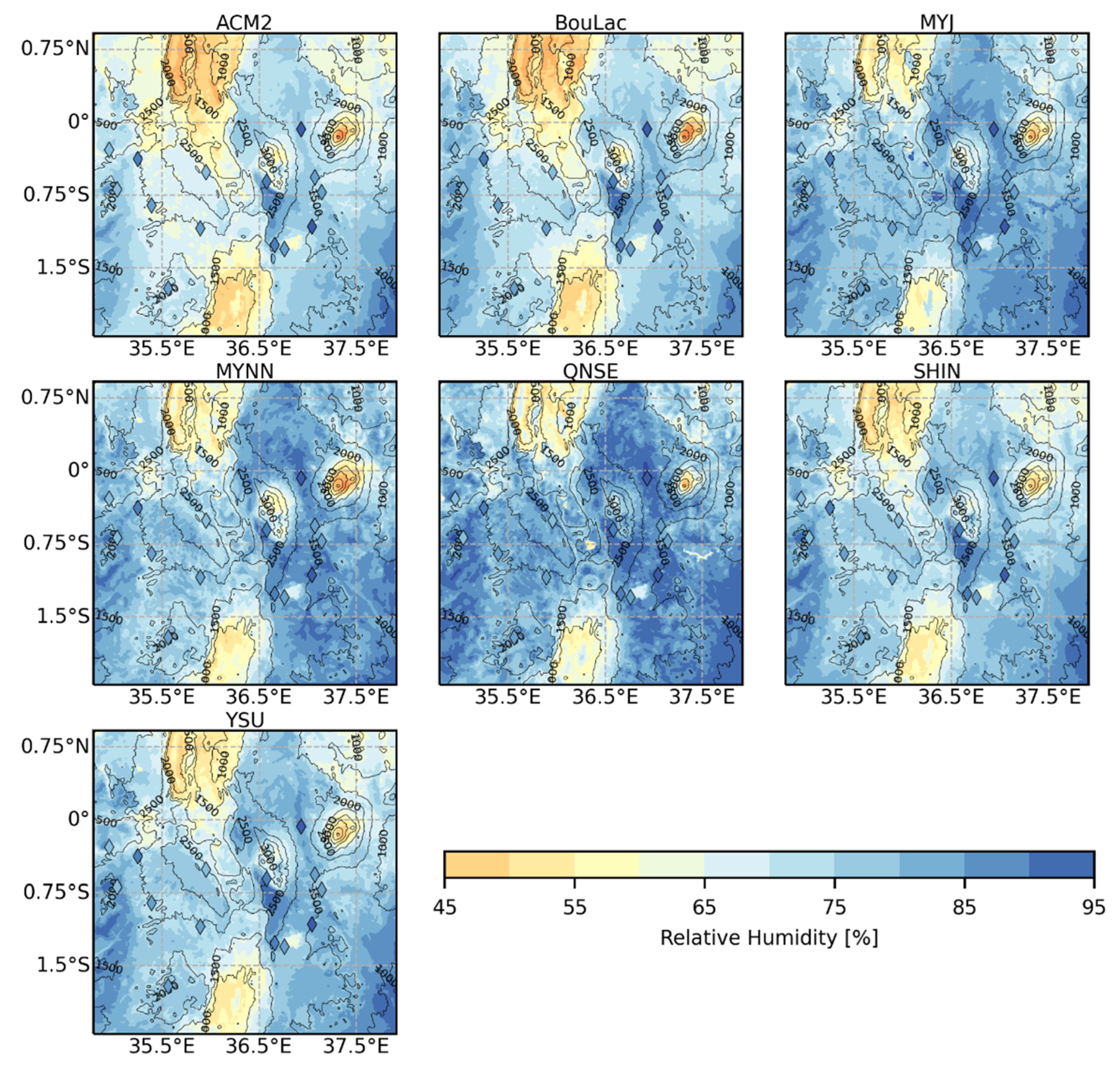
Figure 10 shows the time-averaged RH2 maps at 03:00 UTC (06:00 LT) over the study area. The intra-scheme differences observed in Figure 9 were also apparent in the RH2 maps, particularly with the QNSE scheme, and to a lesser extent, the ACM2 scheme compared to the rest of the schemes. The lower values of RH2 observed with the ACM2 scheme were also discernible in the time-averaged RH2 maps at 11:00 UTC (14:00 LT) in Figure A6 in the Appendix A. The rest of the schemes depicted minimal intra-scheme variations in RH2 at 11:00 UTC (14:00 LT), a trend that is consistent with the trend observed in Figure 9.

The time-averaged vertical profiles of RH at 03:00 UTC (06:00 LT) in Figure 11 show that the local schemes tended to simulate a moister PBL than the nonlocal schemes. However, the local schemes tended to dry up drastically along the vertical atmospheric column compared to the nonlocal schemes. This behavior was more pronounced with the MYNN scheme. It was also observed that at 03:00 UTC (06:00 LT) in Figure 11a (dry season) and Figure 11c (wet season), the BouLac scheme tended to simulate a relatively drier PBL, similar to the nonlocal schemes, compared to the rest of the local schemes. On the other hand, a somewhat drier PBL was simulated by the QNSE scheme at 11:00 UTC (14:00 LT) compared to the rest of the local schemes. The trend observed in the RH profiles was consistent with the trend observed in the RH2 in Figure 9 for most of the schemes across both the wet and dry seasons. One notable difference was that the MYJ scheme simulated a lower RH2 than the QNSE scheme at 03:00 UTC (06:00 LT) despite a relatively more moist PBL at 03:00 UTC (06:00 LT). The significantly lower RH2 observed with ACM2 in Figure 9 was also clearly observed in the RH profiles.

Figure 12 shows the time-averaged diurnal variations in WS10 simulated by the PBL schemes versus the observations. Higher wind speeds were observed during the dry season (Figure 12a) compared to the wet season (Figure 12b) based on both the observations and the WRF simulations. In general, all the PBL schemes overestimated the nighttime WS10 and underestimated the daytime WS10 in both seasons. It was also observed that the SHIN scheme tended to simulate relatively lower daytime WS10 compared to the rest of the schemes. Furthermore, it failed to capture the diurnal variation depicted by the observations, unlike the rest of the schemes. The QNSE and MYJ schemes consistently showed the largest overestimation of the observed WS10 during the day (08:00 (11:00)–14:00 (17:00) UTC (LT)) in both seasons. On the other hand, the ACM2 scheme consistently showed a significant overestimation of the WS10 between 15:00 UTC (18:00 LT) and 20:00 UTC (23:00 LT) in both seasons.

Figure 13 shows the time-averaged maps of WS10 and wind direction at 03:00 UTC (06:00 LT) during the wet season. Just like in Figure 12b, no significant intra-scheme differences were observed in WS10 and the wind direction. Higher wind speeds were observed mainly along mountain slopes. The maps also indicate that wind flow at night is influenced primarily by topography, with no general dominant nighttime wind direction over the study area. Similar patterns were observed in the time-averaged maps of WS10 and wind direction at 03:00 UTC (06:00 LT) during the dry season (Figure A7) in the Appendix A.

Unlike in Figure 13, significant intra-scheme differences consistent with the differences in Figure 12 were observed in the time-averaged maps of WS10 and wind direction at 11:00 UTC (14:00 LT) during the wet season (Figure 14). Strong easterly winds were observed in Figure 14 in most parts of the study area apart from the north, where the winds assumed a more northeasterly direction. On the western side of the study area, some westerly and northwesterly winds, likely blowing from Lake Victoria, were also observed. The large region of low wind speeds observed in the western side of the study area indicates a convergence zone between the prevailing easterly winds and the westerly, northwesterly lake breeze. However, as observed in Figure A8 in the Appendix A, during the dry season, the daytime wind direction predominantly blows from the northeast with the lake breeze, assuming a northerly flow in the western part of the study area for most of the schemes.

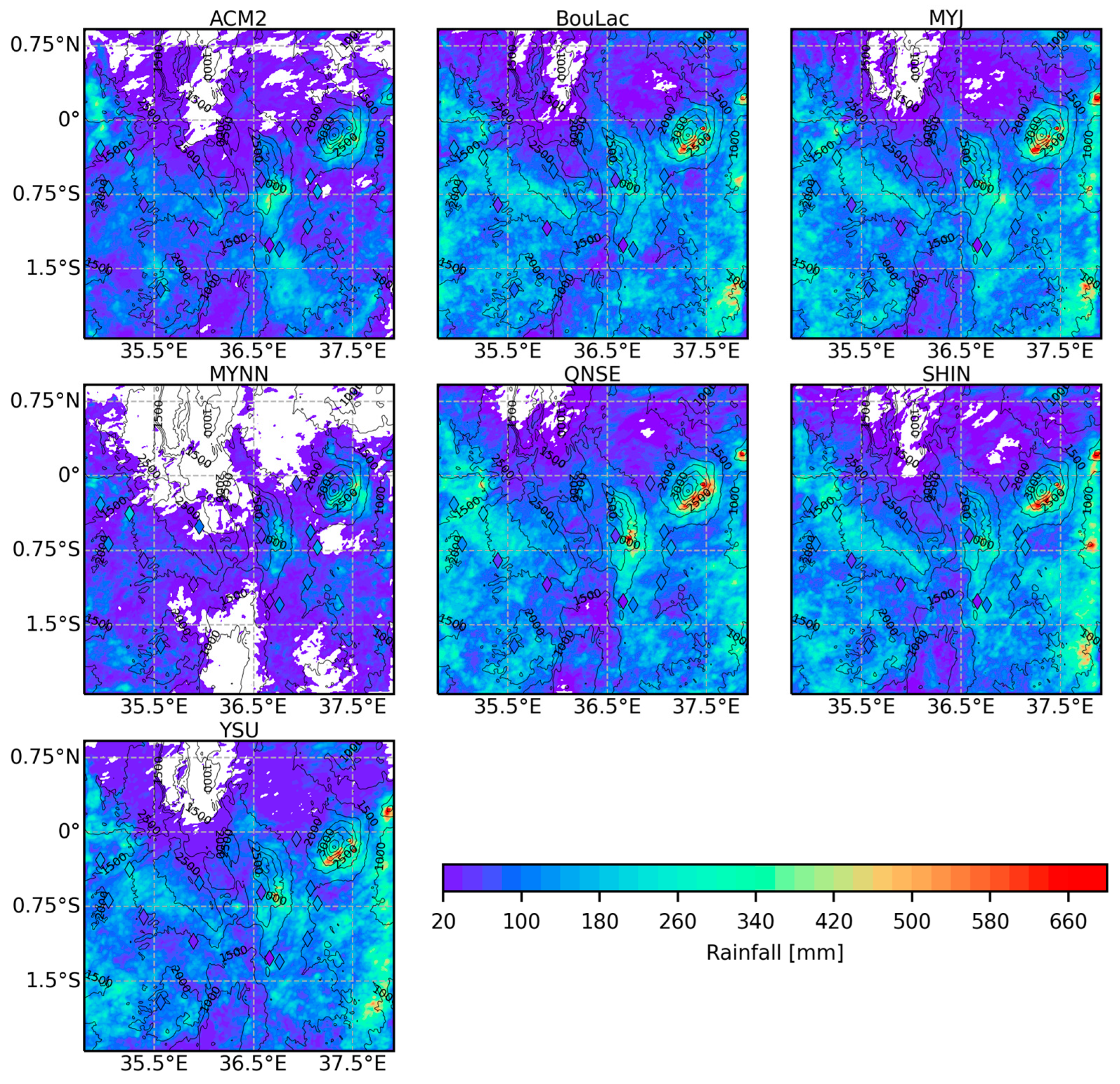
Figure 15 shows the spatial distribution of WRF simulated rainfall using the seven PBL schemes during the wet season. It was observed that the schemes could capture the topography-driven spatial variations in rainfall over the study area. Although the schemes capture the spatial distribution of rainfall depicted by the observations, they tended to overestimate and underestimate the observed rainfall across stations indiscriminately. Additionally, the MYNN and the ACM2 schemes showed slightly lower amounts of rainfall compared to the rest of the schemes. Similar trends were also observed during the dry season in Figure A9 in the Appendix A. However, during the dry season, besides the significantly lower rainfall amounts irrespective of the scheme, the spatial extent of rainfall was mainly restricted to the mountains and the western side of the study area close to Lake Victoria.

Figure 16 shows the probability of occurrence of rain events based on simulations with the various PBL schemes versus the observations. It was observed that the schemes were capable of simulating rainfall events of up to 10 mm/h fairly well. Beyond rainfall intensities of 10 mm/h, the schemes tended to underestimate the intensity of the observed rainfall. The PBL schemes produced similar probability curves, with the main difference being the maximum intensity simulated with each scheme. The MYNN scheme simulated the lowest maximum intensity, approximately 22 mm/h, followed by ACM2 at 24 mm/h. SHIN and BouLac simulated a maximum intensity of approximately 26 mm/h each. The QNSE scheme simulated a maximum intensity of roughly 32 mm/h. The YSU scheme simulated a maximum intensity of approximately 48 mm/h, which is approximately equal to the maximum rainfall event of the observations. The MYJ, on the other hand, simulated a maximum intensity of approximately 54 mm/h, which is beyond the maximum intensity of the observations.

Figure 17 shows the distribution of the ETS values obtained using the seven PBL schemes over the study area during the study period. It was observed that better performances (higher ETS values) were obtained with the YSU scheme followed by the QNSE and BouLac schemes. The MYNN scheme ranked fourth in performance in terms of the ETS. The lowest performance (lower ETS values) was observed with the MYJ scheme, followed by the ACM2 and SHIN schemes, respectively.

4. Discussion

The WRF model has been used in various studies and applications, as reported in Powers et al. [34]. The ability of RCMs such as WRF to add details related to local-scale processes to climate variables derived from GCMs is vital for local climate studies. In addition, it is beneficial for other applications that require high spatial and temporal resolution information on weather and climate, such as energy balance modeling, hydrological applications, among others. As observed in Figure 2, the WRF-simulated T2 shows enhanced spatial details compared to the T2 obtained from ERA5-Land, the highest spatial resolution (9 km) global ReAnalysis dataset currently available for land applications. At the relatively higher spatial resolution of 1 km compared to the 9 km of ERA5-land, the WRF model was able to capture the local scale physical processes related to topography and land use with more details. The refined spatial details captured with the WRF-simulated T2 in Figure 2 imply lower spatial resolution-related biases in the WRF-derived surface meteorological variables than ERA5-land, especially in regions characterized by complex topography. Besides the improved spatial resolution, WRF can simulate variables at higher temporal resolutions than the hourly time scale currently available in ERA5-land.

However, as observed in the statistical results presented in Figure 2 and Figure 3, it is evident that despite the improved spatial resolution achieved through WRF, uncertainties exist in the simulated surface meteorological variables irrespective of the PBL scheme. For instance, it was observed in Figure 6 and Figure 9 that the WRF model generally tends to underestimate T2 and RH2 irrespective of the PBL scheme. Similar findings have been reported in [3,19,21] for T2 and [14,21] RH2. Various other studies have also shown that the WRF model tends to overestimate the observed wind speed [5,19], which agrees with the results presented in Figure 12. One source of uncertainties could be related to uncertainties in the forcing data that might propagate into the WRF simulations. The other source of uncertainties in the simulated surface meteorological variables could be related to the spatial representativeness of the point observations with respect to the 1 km model grid size, especially in complex topography. For instance, the tendency of the WRF model to overestimate wind speed is mainly attributed to the representation of surface roughness in the model, especially in complex environments and at coarser model grid sizes [5], which tends to be smoother, resulting in less resistance. However, it should also be noted that the original observation height of 2 meters might be below the surface roughness height for some of the locations, which might have contributed to lower wind speed at 10 meters upon interpolation using the wind power law. Moreover, the wind power law neglects the effects of surface roughness and atmospheric stability on wind speed. Thus, uncertainties in the observed wind data and the interpolation might have impacted the results.

The choice of a PBL scheme is largely influenced by the weather phenomenon to be studied. Weather phenomena are highly dependent on the state of atmospheric stability. For instance, convective storms occur under extremely unstable atmospheric regimes in which mixing is largely driven by large eddies. On the other hand, under relatively stable atmospheric regimes, mixing is mainly localized and occurs between adjacent layers in the PBL. Local mixing is conducive to the formation of weather phenomena such as fog. Nonlocal PBL schemes are generally better suited for simulating unstable atmospheric regimes, whereas local PBL schemes are more suitable for simulating stable atmospheric regimes. As observed in Figure 8 and Figure 11, the PBL parameterization directly impacts the evolution of the heat and moisture fluxes in the PBL. In general, the local schemes tended to simulate colder, more moist PBLs, especially near the surface relative to the nonlocal schemes. However, the local schemes showed drastic warming and drying with height in the atmospheric column, compared to nonlocal schemes. This implies that the local PBL schemes simulated a more stratified PBL than the nonlocal schemes. The stratification observed with the local schemes was a result of less mixing between the warmer, drier air entrained from the free atmosphere and the cooler, more moist air emanating from the surface. On the other hand, the profiles simulated by the nonlocal schemes in Figure 8 and Figure 11 indicate more mixing between the entrained air mass from the top of the PBL and the air emanating from the surface.

The statistical results presented in Figure 3 and Figure 4 show that choosing a PBL scheme is crucial in retrieving surface meteorological variables using WRF. Although the simulation of T2 and RH2 appear less sensitive to the choice of the PBL scheme, the choice of the PBL scheme will have an impact on the ability of WRF to simulate WS10 and rainfall. These results generally agree with results from other studies [3,19,22,24], which have reported better performances and lower sensitivity to the choice of PBL scheme in WRF in the simulation of T2 and RH2 compared to other surface meteorological variables. The influence of the PBL scheme appears more pronounced during the day when the atmosphere is more convective and unstable than during the night when the atmosphere is relatively stable. The trend observed in the simulated profiles of temperature and humidity (Figure 8 and Figure 11) is propagated to the surface as observed in the plots of T2 and RH2 in Figure 6 and Figure 9, respectively. However, it is observed that in some instances, the trend observed in the profiles of temperature and humidity is not consistent with the trend observed at the surface. An example is at 03:00 UTC (06:00 LT) in Figure 6, where MYJ simulates a relatively higher T2 than QNSE despite similar temperature profiles in Figure 8. These discrepancies may be attributed to differences in the surface layer schemes accompanying each PBL scheme. The influence of the surface layer schemes might also explain the reduced sensitivity observed in T2 and RH2 since the 2-meter height will be mostly within the surface layer, especially under a deep convective PBL. The reduced intra-scheme differences observed in Figure 6 and Figure 9 during the day compared to nighttime further supports this argument.

On the other hand, WS10 and especially rainfall are mainly influenced by the choice of PBL scheme since the heights at which processes related to these variables occur are within the PBL. As observed in Figure 8 and Figure 11, the ACM2 consistently produced a warmer and significantly drier PBL than the rest of the schemes. On the other hand, the MYNN and MYJ schemes simulated a cool and consistently more moist PBL than the rest. The behavior exhibited by the ACM2 and MYJ schemes is reflected in the rainfall probability plots in Figure 16. The ACM2 tends not to capture the higher rainfall intensities, whereas the MYJ scheme simulates some rainfall events that are sometimes way higher than the observations. The behavior observed with the ACM2 and the MYJ schemes in Figure 16 might partly explain the relatively lower ETS values obtained with the two PBL schemes in Figure 17. The results in Figure 16 and Figure 17 imply that the ACM2 scheme might be missing more observed rainfall events than the rest of the schemes. On the other hand, the MYJ scheme might be simulating more false rainfall events than the rest of the schemes. As argued in Coniglio et al. [40] and Cohen et al. [18], nonlocal schemes often tend to simulate too dry of air near the surface owing to PBLs that are too deep and overmixed. Thus, the behavior observed with the ACM2 scheme might be due to a tendency by the scheme to overmix the PBL. On the other hand, local PBL schemes have suffered from undermixing, especially in deep convective environments, mainly due to a poor representation of entrainment processes at the top of the PBL [18], resulting in a shallow, cool, and moist PBL. Thus, MYJ may be susceptible to undermixing in simulating the PBL in this area. Based on the temperature and humidity profiles (Figure 8 and Figure 11) and the rainfall plots in Figure 16 and Figure 17, it appears that the moderately warm and moist PBL profiles simulated by the YSU scheme are more suited for simulating rainfall in this area.

The results presented in Figure 5 also suggest that the model performance might be impacted by the ability of the PBL schemes to represent the interactions between the large-scale and local-scale processes. As observed in Figure 14 and Figure A8, during the day, processes in the western side close to Lake Victoria are influenced by the interaction between the more large-scale wind flows from the eastern side and the lake breeze. Thus, improper representation of the interactions between the two air masses might explain the higher RMSE values for the RH2 observed in the western side of the study area in Figure 5. For instance, the location of the convergence zone observed in Figure 14 will be highly influenced by the ability of the schemes to properly simulate the direction and strength of the lake breeze and its interaction with the prevailing wind flow. In addition, the ability of the PBL scheme to represent local-scale turbulence related to land use and topography and its interaction with the large-scale processes, such as the prevailing wind flow, will have a significant impact on the performance of the model. As observed in Figure 14 and Figure A8, intra-scheme differences in wind speed are quite pronounced during the day, as opposed to during the night (Figure 13 and Figure A7). The daytime intra-scheme differences in wind speed signify the differences in the ability of the various PBL schemes to represent buoyancy and vertical wind shear related to the interaction between the local scale turbulence and the larger-scale wind flow in the PBL. All these interactions influence the wind speed and direction and the distribution of moisture within the atmosphere. Consequently, other processes such as convection will be affected by these interactions impacting the simulated rainfall. As such, the effectiveness of the parameterizations in the PBL scheme in representing such interactions will determine the scheme’s success in representing the local-scale processes.

Although the 2-meter variables appear less sensitive to the choice of the PBL scheme in this study, the choice of a PBL scheme for studies involving 2-meter variables is still essential. As observed in Figure 8 and Figure 11, the representation of fluxes along the vertical profile can vary significantly depending on the PBL scheme. Under extreme conditions, such as heatwaves, large eddy-driven turbulent mixing will be dominant across the PBL, significantly influencing the 2-meter variables as well. As such, modeling of the PBL should be carefully considered even for studies involving 2-meter variables.

5. Conclusions

This study evaluated the influence of PBL parameterization schemes in WRF in the retrieval of surface meteorological variables over the Kenyan highlands. The experimental setup was configured into three one-way nested model domains, with the innermost domain being at a spatial resolution of 1 km. The model was driven by forcing data from ERA5 at six hourly intervals. The study evaluated seven PBL schemes, namely: ACM2, BouLac, MYJ, MYNN, QNSE, SHIN, and YSU. The evaluation was only carried out for the innermost model domain. The surface meteorological variables considered are the T2, RH2, WS10, and rainfall. The surface meteorological variables were validated against observations from TAHMO.

In general, WRF was found to simulate surface meteorological variables that exhibited spatial variability consistent with the complex topography within the Kenyan highlands. A comparison between T2 simulated by WRF and T2 obtained from ERA5-Land revealed more spatial details with WRF than ERA5. Thus, WRF-derived surface meteorological variables are better suited for land applications within the Kenyan highlands than ERA-5 land.

On the influence of PBL schemes on surface meteorological variables, it was observed that T2 and RH2 are less sensitive to the PBL scheme’s choice than WS10 and rainfall. T2 and RH2 are less sensitive to the choice of the PBL owing partly to the influence of the surface layer parameterization on these variables. Since the processes related to rainfall mainly occur in the PBL, we conclude that rainfall better reflects the influence of the PBL schemes. Thus, based on the results of the simulated rainfall, the YSU scheme provides a more realistic depiction of the PBL dynamics within the study area.

One of the limitations to this study is the lack of observations of fluxes along the vertical profile, which hinders a comprehensive evaluation of PBL dynamics within the study area. Additionally, the study considered only a period of four months owing to limitations in computation resources. This period may be inadequate, especially in the evaluation of the seasonal dynamics within the study area.

Future studies should incorporate observations on the atmospheric profile. The studies should also consider simulations over more extended periods to determine the influence of seasonality on the model performance within the study area.

References

1. Giorgi, F. Thirty Years of Regional Climate Modeling: Where Are We and Where Are We Going next? J. Geophys. Res. Atmos. 2019, 124, 5696–5723. [Google Scholar] [CrossRef] [Green Version]
2. Feser, F.; Rrockel, B.; Storch, H.; Winterfeldt, J.; Zahn, M. Regional climate models add value to global model data a review and selected examples. Bull. Am. Meteorol. Soc. 2011, 92, 1181–1192. [Google Scholar] [CrossRef] [Green Version]
3. García-Díez, M.; Fernández, J.; Fita, L.; Yagüe, C. Seasonal dependence of WRF model biases and sensitivity to PBL schemes over Europe. Q. J. R. Meteorol. Soc. 2013, 139, 501–514. [Google Scholar] [CrossRef] [Green Version]
4. Dasari, H.P.; Salgado, R.; Perdigao, J.; Challa, V.S. A Regional Climate Simulation Study Using WRF-ARW Model over Europe and Evaluation for Extreme Temperature Weather Events. Int. J. Atmos. Sci. 2014, 2014, 1–22. [Google Scholar] [CrossRef] [Green Version]
5. Zhang, H.; Pu, Z.; Zhang, X. Examination of errors in near-surface temperature and wind from WRF numerical simulations in regions of complex terrain. Weather Forecast. 2013, 28, 893–914. [Google Scholar] [CrossRef] [Green Version]
6. Stensrud, D.J. Parameterization Schemes: Keys to Understanding Numerical Weather Prediction Models; Cambridge University Press: Cambridge, UK, 2007; ISBN 9780521126762. [Google Scholar]
7. Otieno, G.; Mutemi, J.N.; Opijah, F.J.; Ogallo, L.A.; Omondi, M.H. The Sensitivity of Rainfall Characteristics to Cumulus Parameterization Schemes from a WRF Model. Part I: A Case Study Over East Africa During Wet Years. Pure Appl. Geophys. 2020, 177, 1095–1110. [Google Scholar] [CrossRef]
8. Pei, L.; Moore, N.; Zhong, S.; Luo, L.; Hyndman, D.W.; Heilman, W.E.; Gao, Z. WRF model sensitivity to land surface model and cumulus parameterization under short-term climate extremes over the Southern great plains of the United States. J. Clim. 2014, 27, 7703–7724. [Google Scholar] [CrossRef]
9. Shepherd, T.J.; Walsh, K.J. Sensitivity of hurricane track to cumulus parameterization schemes in the WRF model for three intense tropical cyclones: Impact of convective asymmetry. Meteorol. Atmos. Phys. 2017, 129, 345–374. [Google Scholar] [CrossRef]
10. Martínez-Castro, D.; Kumar, S.; Flores Rojas, J.L.; Moya-Álvarez, A.; Valdivia-Prado, J.M.; Villalobos-Puma, E.; Castillo-Velarde, C.D.; Silva-Vidal, Y. The Impact of Microphysics Parameterization in the Simulation of Two Convective Rainfall Events over the Central Andes of Peru Using WRF-ARW. Atmosphere 2019, 10, 442. [Google Scholar] [CrossRef] [Green Version]
11. Dawn, S.; Satyanarayana, A.N.V. Sensitivity studies of cloud microphysical schemes of WRF-ARW model in the simulation of trailing stratiform squall lines over the Gangetic West Bengal region. J. Atmos. Solar-Terrestrial Phys. 2020, 209, 105396. [Google Scholar] [CrossRef]
12. Sikder, M.S.; Hossain, F. Sensitivity of initial-condition and cloud microphysics to the forecasting of monsoon rainfall in South Asia. Meteorol. Appl. 2018, 25, 493–509. [Google Scholar] [CrossRef] [Green Version]
13. Li, X.; Pu, Z. Sensitivity of numerical simulation of early rapid intensification of Hurricane Emily (2005) to cloud microphysical and planetary boundary layer parameterizations. Mon. Weather Rev. 2008, 136, 4819–4838. [Google Scholar] [CrossRef]
14. Avolio, E.; Federico, S.; Miglietta, M.M.; Lo Feudo, T.; Calidonna, C.R.; Sempreviva, A.M. Sensitivity analysis of WRF model PBL schemes in simulating boundary-layer variables in southern Italy: An experimental campaign. Atmos. Res. 2017, 192, 58–71. [Google Scholar] [CrossRef]
15. Shin, H.H.; Hong, S.Y. Intercomparison of Planetary Boundary-Layer Parametrizations in the WRF Model for a Single Day from CASES-99. Bound.-Layer Meteorol. 2011, 139, 261–281. [Google Scholar] [CrossRef]
16. Hong, S.Y.; Pan, H.L. Nonlocal boundary layer vertical diffusion in a medium-range forecast model. Mon. Weather Rev. 1996, 124, 2322–2339. [Google Scholar] [CrossRef] [Green Version]
17. Braun, S.A.; Tao, W.K. Sensitivity of high-resolution simulations of Hurricane Bob (1991) to planetary boundary layer parameterizations. Mon. Weather Rev. 2000, 128, 3941–3961. [Google Scholar] [CrossRef] [Green Version]
18. Cohen, A.E.; Cavallo, S.M.; Coniglio, M.C.; Brooks, H.E. A review of planetary boundary layer parameterization schemes and their sensitivity in simulating southeastern U.S. cold season severe weather environments. Weather Forecast. 2015, 30, 591–612. [Google Scholar] [CrossRef]
19. Banks, R.F.; Tiana-Alsina, J.; Baldasano, J.M.; Rocadenbosch, F.; Papayannis, A.; Solomos, S.; Tzanis, C.G. Sensitivity of boundary-layer variables to PBL schemes in the WRF model based on surface meteorological observations, lidar, and radiosondes during the HygrA-CD campaign. Atmos. Res. 2016, 176–177, 185–201. [Google Scholar] [CrossRef]
20. Hazra, V.; Pattnaik, S. Systematic errors in the WRF model planetary boundary layer schemes for two contrasting monsoon seasons over the state of Odisha and its neighborhood region. Theor. Appl. Climatol. 2020, 139, 1079–1096. [Google Scholar] [CrossRef]
21. Boadh, R.; Satyanarayana, A.N.V.; Rama Krishna, T.V.B.P.S.; Madala, S. Sensitivity of PBL schemes of the WRF-ARW model in simulating the boundary layer flow parameters for their application to air pollution dispersion modeling over a tropical station. Atmosfera 2016, 29, 61–81. [Google Scholar] [CrossRef] [Green Version]
22. Chaouch, N.; Temimi, M.; Weston, M.; Ghedira, H. Sensitivity of the meteorological model WRF-ARW to planetary boundary layer schemes during fog conditions in a coastal arid region. Atmos. Res. 2017, 187, 106–127. [Google Scholar] [CrossRef]
23. Ooi, M.C.G.; Chan, A.; Kumarenthiran, S.; Morris, K.I.; Oozeer, M.Y.; Islam, M.A.; Salleh, S.A. Comparison of WRF local and nonlocal boundary layer Physics in Greater Kuala Lumpur, Malaysia. In Proceedings of the IOP Conference Series: Earth and Environmental Science; Institute of Physics Publishing: Selangor, Malaysia, 2018; Volume 117, p. 012015. [Google Scholar]
24. Tyagi, B.; Magliulo, V.; Finardi, S.; Gasbarra, D.; Carlucci, P.; Toscano, P.; Zaldei, A.; Riccio, A.; Calori, G.; D’Allura, A.; et al. Performance Analysis of Planetary Boundary Layer Parameterization Schemes in WRF Modeling Set Up over Southern Italy. Atmosphere 2018, 9, 272. [Google Scholar] [CrossRef] [Green Version]
25. Madala, S.; Satyanarayana, A.N.V.; Srinivas, C.V.; Tyagi, B. Performance Evaluation of PBL Schemes of ARW Model in Simulating Thermo-Dynamical Structure of Pre-Monsoon Convective Episodes over Kharagpur Using STORM Data Sets. Pure Appl. Geophys. 2016, 173, 1803–1827. [Google Scholar] [CrossRef]
26. Gbode, I.E.; Dudhia, J.; Ogunjobi, K.O.; Ajayi, V.O. Sensitivity of different physics schemes in the WRF model during a West African monsoon regime. Theor. Appl. Climatol. 2019, 136, 733–751. [Google Scholar] [CrossRef] [Green Version]
27. de Lange, A.; Naidoo, M.; Garland, R.M.; Dyson, L.L. The sensitivity of simulated surface-level pollution concentrations to WRF-ARW-model PBL parameterisation schemes over the Highveld of South Africa. Atmos. Res. 2021, 254, 105517. [Google Scholar] [CrossRef]
28. Yang, B.; Berg, L.K.; Qian, Y.; Wang, C.; Hou, Z.; Liu, Y.; Shin, H.H.; Hong, S.; Pekour, M. Parametric and Structural Sensitivities of Turbine-Height Wind Speeds in the Boundary Layer Parameterizations in the Weather Research and Forecasting Model. J. Geophys. Res. Atmos. 2019, 124, 5951–5969. [Google Scholar] [CrossRef] [Green Version]
29. Mcdowell, G.; Ford, J.; Jones, J. Community-level climate change vulnerability research: Trends, progress, and future directions. Environ. Res. Lett. 2016, 11, 033001. [Google Scholar] [CrossRef]
30. Gebrechorkos, S.H.; Hülsmann, S.; Bernhofer, C. Regional climate projections for impact assessment studies in East Africa. Environ. Res. Lett. 2019, 14, 044031. [Google Scholar] [CrossRef]
31. Van De Giesen, N.; Annor, F.O.; Hochreutener, R.; Selker, J.S.; Van De Giesen, N.; Annor, F.O.; Hochreutener, R.; Selker, J.S. The first five years of the Trans-African Hydro-Meteorological observatory (TAHMO): From nice idea to a network of 500+ stations. AGUFM 2019, 2019, H44D-05. [Google Scholar]
32. Argent, R.; Sun, X.; Semazzi, F.; Xie, L.; Liu, B. The development of a customization framework for the WRF model over the lake Victoria basin, eastern Africa on seasonal timescales. Adv. Meteorol. 2015, 2015, 653473. [Google Scholar] [CrossRef] [Green Version]
33. Kerandi, N.; Arnault, J.; Laux, P.; Wagner, S.; Kitheka, J.; Kunstmann, H. Joint atmospheric-terrestrial water balances for East Africa: A WRF-Hydro case study for the upper Tana River basin. Theor. Appl. Climatol. 2018, 131, 1337–1355. [Google Scholar] [CrossRef] [Green Version]
34. Powers, J.G.; Klemp, J.B.; Skamarock, W.C.; Davis, C.A.; Dudhia, J.; Gill, D.O.; Coen, J.L.; Gochis, D.J.; Ahmadov, R.; Peckham, S.E.; et al. The weather research and forecasting model: Overview, system efforts, and future directions. Bull. Am. Meteorol. Soc. 2017, 98, 1717–1737. [Google Scholar] [CrossRef]
35. Kong, J.; Zhao, Y.; Carmeliet, J.; Lei, C. Urban heat island and its interaction with heatwaves: A review of studies on mesoscale. Sustain. 2021, 13, 10923. [Google Scholar] [CrossRef]
36. Janjic, Z.I. A nonhydrostatic model based on a new approach. Meteorol. Atmos. Phys. 2003, 82, 271–285. [Google Scholar] [CrossRef]
37. Skamarock, W.C.; Klemp, J.B.; Dudhi, J.; Gill, D.O.; Barker, D.M.; Duda, M.G.; Huang, X.-Y.; Wang, W.; Powers, J.G. A Description of the Advanced Research WRF Version 3; 2008. Available online: https://opensky.ucar.edu/islandora/object/technotes:500 (accessed on 2 December 2021).
38. Pleim, J.E. A combined local and nonlocal closure model for the atmospheric boundary layer. Part I: Model description and testing. J. Appl. Meteorol. Climatol. 2007, 46, 1383–1395. [Google Scholar] [CrossRef]
39. Pleim, J.E. A combined local and nonlocal closure model for the atmospheric boundary layer. Part II: Application and evaluation in a mesoscale meteorological model. J. Appl. Meteorol. Climatol. 2007, 46, 1396–1409. [Google Scholar] [CrossRef] [Green Version]
40. Coniglio, M.C.; Correia, J.; Marsh, P.T.; Kong, F. Verification of convection-allowing WRF model forecasts of the planetary boundary layer using sounding observations. Weather Forecast. 2013, 28, 842–862. [Google Scholar] [CrossRef]
41. Bougeault, P.; Lacarrere, P. Parameterization of orography-induced turbulence in a mesobeta-scale model. Mon. Weather Rev. 1989, 117, 1872–1890. [Google Scholar] [CrossRef]
42. Janjić, Z.I. Nonsingular Implementation of the Mellor-Yamada Level 2.5 Scheme in the NCEP Meso Model, 2001. Available online: https://repository.library.noaa.gov/view/noaa/11409 (accessed on 2 December 2021).
43. Nakanishi, M.; Niino, H. An improved Mellor-Yamada Level-3 model: Its numerical stability and application to a regional prediction of advection fog. Bound.-Layer Meteorol. 2006, 119, 397–407. [Google Scholar] [CrossRef]
44. Nakanishi, M.; Niino, H. An improved Mellor-Yamada Level-3 model with condensation physics: Its design and verification. Bound.-Layer Meteorol. 2004, 112, 1–31. [Google Scholar] [CrossRef]
45. Sukoriansky, S.; Galperin, B.; Perov, V. Application of a new spectral theory of stably stratified turbulence to the atmospheric boundary layer over sea ice. Bound.-Layer Meteorol. 2005, 117, 231–257. [Google Scholar] [CrossRef]
46. Shin, H.H.; Hong, S.Y. Representation of the subgrid-scale turbulent transport in convective boundary layers at gray-zone resolutions. Mon. Weather Rev. 2015, 143, 250–271. [Google Scholar] [CrossRef]
47. Shin, H.H.; Hong, S.Y. Analysis of resolved and parameterized vertical transports in convective boundary layers at gray-zone resolutions. J. Atmos. Sci. 2013, 70, 3248–3261. [Google Scholar] [CrossRef]
48. Hong, S.Y.; Noh, Y.; Dudhia, J. A new vertical diffusion package with an explicit treatment of entrainment processes. Mon. Weather Rev. 2006, 134, 2318–2341. [Google Scholar] [CrossRef] [Green Version]
49. Nicholson, S.E. Climate and climatic variability of rainfall over eastern Africa. Rev. Geophys. 2017, 55, 590–635. [Google Scholar] [CrossRef] [Green Version]
50. Jiménez, P.A.; Dudhia, J.; González-Rouco, J.F.; Navarro, J.; Montávez, J.P.; García-Bustamante, E. A revised scheme for the WRF surface layer formulation. Mon. Weather Rev. 2012, 140, 898–918. [Google Scholar] [CrossRef] [Green Version]
51. Janjic, Z.I. The step-mountain eta coordinate model: Further developments of the convection, viscous sublayer, and turbulence closure schemes. Mon. Weather Rev. 1994, 122, 927–945. [Google Scholar] [CrossRef] [Green Version]
52. Hong, S.Y.; Dudhia, J.; Chen, S.H. A revised approach to ice microphysical processes for the bulk parameterization of clouds and precipitation. Mon. Weather Rev. 2004, 132, 103–120. [Google Scholar] [CrossRef]
53. Dudhia, J. Numerical study of convection observed during the Winter Monsoon Experiment using a mesoscale two-dimensional model. J. Atmos. Sci. 1989, 46, 3077–3107. [Google Scholar] [CrossRef]
54. Mlawer, E.J.; Taubman, S.J.; Brown, P.D.; Iacono, M.J.; Clough, S.A. Radiative transfer for inhomogeneous atmospheres: RRTM, a validated correlated-k model for the longwave. J. Geophys. Res. Atmos. 1997, 102, 16663–16682. [Google Scholar] [CrossRef] [Green Version]
55. Chen, F.; Dudhia, J. Coupling and advanced land surface-hydrology model with the Penn State-NCAR MM5 modeling system. Part I: Model implementation and sensitivity. Mon. Weather Rev. 2001, 129, 569–585. [Google Scholar] [CrossRef] [Green Version]
56. Hogan, R.J.; Ferro, C.A.T.; Jolliffe, I.T.; Stephenson, D.B. Equitability revisited: Why the “equitable threat score” is not equitable. Weather Forecast. 2010, 25, 710–726. [Google Scholar] [CrossRef] [Green Version]
Figure 1. WRF Model domain configurations (a) and the study area corresponding to the inner model domain showing the location of the weather stations within the study area (b). The horizontal resolutions of the model domains, D01, D02, and D03, are 9, 3, and 1 km, respectively.
Atmosphere 13 00169 g001
Figure 2. T2 contour map derived with the YSU scheme for the inner model domain at 1 km grid resolution (a) and T2 contour map obtained from ERA5 at 9 km grid resolution (b), both corresponding to 20 January 2019 at 08:00 UTC (11:00 LT), superimposed with the observed 2-meter air temperature.
Atmosphere 13 00169 g002
Figure 3. PDF plots showing the distribution of the correlation coefficient (R) values obtained using the seven PBL schemes for T2 (a), RH (b), WS10 (c), and rainfall (d) across all the observation stations during the entire study period, excluding the 5 days set aside for model spin-up.
Atmosphere 13 00169 g003
Figure 4. PDF plots showing the distribution of the RMSE values obtained using the seven PBL schemes for T2 (a), RH (b), WS10 (c), and rainfall (d) across all of the observation stations during the entire study period, excluding the 5 days set aside for model spin-up.
Atmosphere 13 00169 g004
Figure 5. Spatial distribution of RMSE values for the 2-meter relative humidity (RH2) obtained using the seven PBL schemes across the observation stations over the entire study period, excluding the 5 days set aside for model spin-up.
Atmosphere 13 00169 g005
Figure 6. Time-averaged diurnal variation of the 2-meter air temperature (T2) simulated with the seven PBL schemes compared to the observations during the dry season (a) and wet season (b). Time (UTC) corresponds to UTC +3 hours local time (LT) for the study area.
Atmosphere 13 00169 g006
Figure 7. Time-averaged maps of simulated 2-meter air temperature (T2) for the inner model domain (1 km grid resolution) at 03:00 UTC (06:00 LT) using the seven PBL schemes during the entire study period, excluding the 5 days set aside for model spin-up.
Atmosphere 13 00169 g007
Figure 8. Time-averaged vertical profiles of potential temperature corresponding to 03:00 UTC (06:00 LT) for the dry season (a) and the wet season (c), and corresponding to 11:00 UTC (14:00 LT) for the dry season (b) and the wet season (d), as simulated by each of the seven PBL schemes.
Atmosphere 13 00169 g008
Figure 9. Time-averaged diurnal variation of the 2-meter relative humidity (RH2) simulated with the seven PBL schemes compared to the observations during the dry season (a) and wet season (b). Time (UTC) corresponds to UTC +3 hours local time (LT) for the study area.
Atmosphere 13 00169 g009
Figure 10. Time-averaged maps of the simulated 2-meter relative humidity (RH2) for the inner model domain (1 km grid resolution) at 03:00 UTC (06:00 LT) using the seven PBL schemes during the entire study period.
Atmosphere 13 00169 g010
Figure 11. Time-averaged vertical profiles of relative humidity corresponding to 03:00 UTC (06:00 LT) for the dry season (a) and the wet season (c), and corresponding to 11:00 UTC (14:00 LT) for the dry season (b) and the wet season (d), as simulated by each of the seven PBL schemes.
Atmosphere 13 00169 g011
Figure 12. Time-averaged diurnal variation of 10-meter wind speed (WS10) simulated with the seven PBL schemes compared to the observations during the dry season (a) and wet season (b). Time (UTC) corresponds to UTC +3 hours local time (LT) for the study area.
Atmosphere 13 00169 g012
Figure 13. Time-averaged maps of the simulated 10-meter wind speed (WS10) and wind direction for the inner model domain (1 km grid resolution) at 03:00 UTC (06:00 LT) using the seven PBL schemes and the corresponding time-averaged observed WS10 and wind direction during the wet season. The circle on the wind barb represents calm winds with speeds of up to 2 km/h. A straight line without a barb represents wind speeds between 2 and 4 km/h. A short barb represents wind speeds ranging between 5 and 14 km/h, whereas a long barb represents wind speeds ranging between 15 and 23 km/h. Higher wind speeds are represented by a combination of short and long barbs.
Atmosphere 13 00169 g013
Figure 14. Time-averaged maps of the simulated 10-meter wind speed (WS10) and wind direction for the inner model domain (1km grid resolution) at 11:00 UTC (14:00 LT) using the seven PBL schemes and the corresponding time-averaged observed WS10 and wind direction during the wet season. The circle on the wind barb represents calm winds with speeds of up to 2 km/h. A straight line without a barb represents wind speeds between 2 and 4 km/h. A short barb represents wind speeds ranging between 5 and 14 km/h, whereas a long barb represents wind speeds ranging between 15 and 23 km/h. Higher wind speeds are represented by a combination of short and long barbs.
Atmosphere 13 00169 g014
Figure 15. Maps of accumulated rainfall for the inner model domain (1 km grid resolution) during the wet season from the seven PBL schemes superimposed with the accumulated observed rainfall during the same period. The white color on the maps represents areas with no rainfall.
Atmosphere 13 00169 g015
Figure 16. Plot showing the probability of capturing observed hourly rainfall events based on the seven PBL schemes.
Atmosphere 13 00169 g016
Figure 17. PDF plots showing the distribution of the Equitable Threat Score (ETS) values for rainfall obtained using the seven PBL schemes over the study area during the entire study period, excluding the 5 days set aside for model spin-up.
Atmosphere 13 00169 g017