Properties of Magnetic Field Fluctuations in Long-Lasting Radial IMF Events from Wind Observation

Abstract

Long-lasting radial interplanetary magnetic field (IMF) intervals in which IMF points along the solar wind velocity for several hours have many interesting properties. We investigate the average parameters and the behavior of magnetic field fluctuations within 419 such radial intervals. The power spectral density (PSD) calculated over 1-h intervals of a radial IMF is compared with PSDs in adjacent regions prior to and after the radial IMF. We concentrate on (1) the power of IMF fluctuations, (2) the median slopes of PSDs in both inertial and kinetic ranges, (3) the proton temperature and its anisotropy, and (4) the occurrence rate of wavy structures and their polarization. We have shown that the fluctuation amplitude is low in the radial IMF intervals in both magnetohydrodynamic (MHD) and kinetic ranges, and the spectral power increases with the cone angle in the MHD range. We discuss this effect in the light of present knowledge on plasma turbulence and peculiarities of observations of magnetic field variations under the radial background magnetic field. We found that in the radial IMF events, the proton temperature is more isotropic, the occurrence rate of waves is higher, and the waves have no preferred polarization in the frequency range from 0.1 to 1 Hz. It suggests that the radial IMF structure leads to a different development of turbulence than the typical Parker-spiral structure.

1. Introduction

The interplanetary magnetic field (IMF) strength and orientation play a critical role in many space processes. For example, the IMF orientation controls solar wind thermal characteristics, enhancements in the IMF strength are effective in excluding low-energy cosmic rays from the solar system, energetic particles from the Sun are guided outward into interplanetary space along the IMF lines, and the solar wind parameters, including the fluctuation amplitude, also change with this orientation. Moreover, the IMF is one of the most important parameters affecting space weather because it modifies the solar wind interaction with magnetized planets. The past studies have shown that the IMF component perpendicular to the ecliptic plane determines to a high degree the magnetospheric response to upstream variations, such as the size and shape of the magnetopause [1,2], the magnetospheric dynamics [3,4], the waves in the magnetosphere [5], etc. For these reasons, the influence of south- and northward IMF on the magnetospheric system has been intensively studied in the past four decades.

On the other hand, the radial IMF orientation started to attract the attention of the scientific community. The radial component also plays an important role, e.g., in space weather, the location and shape of the magnetopause, some bow shock effects, and in processes connecting with a formation of the dayside magnetopause and adjacent layers [6]. The radial IMF is the special solar wind condition when the IMF orientation is aligned with the solar wind flow (the angle between the velocity direction and mean magnetic field direction, θ_BV ≤ 30°), and such a situation can be stable for several hours. Within long-duration radial IMF intervals, the solar wind parameters are characterized by a weak magnetic field strength, a low density of the cold plasma, and small fluctuations of all solar wind parameters in comparison with their yearly averages [7]. Gosling & Skoug [8] proposed a simple model to explain the formation of radial IMF. The solar wind streams with different bulk speeds stretch the magnetic field on two sides of the same magnetic field line. Schwadron [9] suggested a different model of the origin of radial IMF events related to the magnetic foot-point motion at the source surface. However, the bulk speed difference is also the main factor creating the radial field in this model.

The θ_BV angle plays an essential role in the setting solar wind characteristics. For instance, magnetic helicity in the solar wind has an θ_BV dependence; positive magnetic helicity appears at a large θ_BV (around 90°), whereas negative magnetic helicity prefers a small angle [10]. In addition, the behavior of fluctuations in the solar wind is related to θ_BV. The power-law index of the Power Spectral Density (PSD) of the magnetic field in the inertial range of frequencies varies from −5/3 to −2 when θ_BV decreases from 90° to 0° [11]. This result was later confirmed in the study of both high- and low-latitude high-speed streams [12]. In the same study, the observations revealed that the power of fluctuations is higher when θ_BV is around 90° and weaker when θ_BV is small. The difference between 90° and 0° is approximately a factor of 2 at 0.01 Hz. Using Parker Solar Probe measurements, Duan et al. [13] showed that the PSD slopes in the near solar region vary with θ_BV. The slopes are steeper when θ_BV turns to a nearly radial direction. Particularly, in the kinetic range, the slopes change from −3.60 when the IMF is perpendicular to the solar wind flow to −6.79 when it is parallel to the solar wind flow. These angular dependencies are interpreted by power and spectral index anisotropies, and this feature becomes important in interpreting the energy cascade processes in solar wind turbulence [14,15,16,17,18]. A brief explanation of angular dependence is based on the fact that the perpendicular and parallel fluctuations have different properties, and a mixture is observed when the sampling angle is oblique.

One of the major tasks in studying those angular dependences is determination of the local background magnetic field direction in a highly fluctuating IMF. Previous studies are usually based on regular solar wind structures such as high-speed streams, and they define the local background magnetic field direction as the mean magnetic field in the selected time window [17]. However, when the IMF fluctuations are large and contain a significant portion of low-frequency variations, the mean local magnetic field does not necessarily represent the entire window, e.g., [19]. To fix this problem, Wu et al. [16] divided the whole interval under question into two equal halves and calculated the average magnetic field within them. They then select only intervals with the angle between mean magnetic fields in these two halves lower than 10° to exclude the uncertainty of a background magnetic field direction caused by the large-scale variations.

The stable and highly aligned solar wind flow direction within long-lasting (several hours) radial IMF intervals provides optimal conditions for the study of parallel fluctuations in the solar wind, and thus we selected such events in Wind observations during 1995 to 2018. The long duration of the radial IMF orientation could lead to the different behavior of fluctuations than the short IMF turns to radial orientation [20,21]. For example, Telloni et al. [22] point out that they did not find evidence for a critical balance in the field-aligned solar wind. The following section describes the data and the selection criteria for the identification of long-lasting radial IMF events. The results of their analysis are the subject of Section 3, and the discussion and conclusions are presented in Section 4 and Section 5, respectively.

2. Data

The Wind spacecraft was launched on 1 November 1994 and has orbited around the L1 point since 2004 to monitor solar wind conditions continuously. The plasma data recorded by the Solar Wind Experiment with a 92-s resolution (SWE; [23]) are used to identify the plasma characteristics in this study. The Magnetic Field Investigation device (MFI; [24]) provides the high resolution (0.092 s) magnetic field vector applied for study of the magnetic field fluctuations.

The criteria for long-lasting radial IMF intervals are adapted from Pi et al. [7]. The ratio of the B_x magnetic field component and its magnitude should be larger than 0.9 ($\raisebox{1ex}{$\left|{\mathit{B}}_{\mathit{x}}\right|$}\!\left/ \!\raisebox{-1ex}{$\mathit{B}$}\right.\ge \mathbf{0.9}$) for four or more hours, but a short break (less than 15 min) is allowed. Hereafter, we use the ratio ($\raisebox{1ex}{$\left|{\mathit{B}}_{\mathit{x}}\right|$}\!\left/ \!\raisebox{-1ex}{$\mathit{B}$}\right.$) instead of θ_BV because the solar wind propagates nearly radially, and thus these two quantities carry similar information. Pi et al. [7] used a 6-h lasting interval as the criterion because the authors assumed that only large structures have a clear solar source. On the other hand, we only need a stationary IMF direction regardless of the source, and thus a 4-h lasting interval is sufficient for our study.

A total of 419 intervals of different duration passing the above conditions were identified in the solar wind, and Figure 1 shows an example of such an interval. Two vertical dashed lines denote the starting and ending times of the interval under question, and the ratio of $\raisebox{1ex}{$\left|{\mathit{B}}_{\mathit{x}}\right|$}\!\left/ \!\raisebox{-1ex}{$\mathit{B}$}\right.$, magnitude and magnetic field vector, bulk proton speed V_p, V_Y and V_Z components of the proton velocity, proton number density, proton parallel and perpendicular thermal velocities, and temperature anisotropy are presented from top to bottom. Compared with the highly fluctuating value in the adjacent regions, $\raisebox{1ex}{$\left|{\mathit{B}}_{\mathit{x}}\right|$}\!\left/ \!\raisebox{-1ex}{$\mathit{B}$}\right.$ stays over 0.9 for the whole 7-interval, and all other solar wind parameters are also highly stable in the whole interval.

3. Results

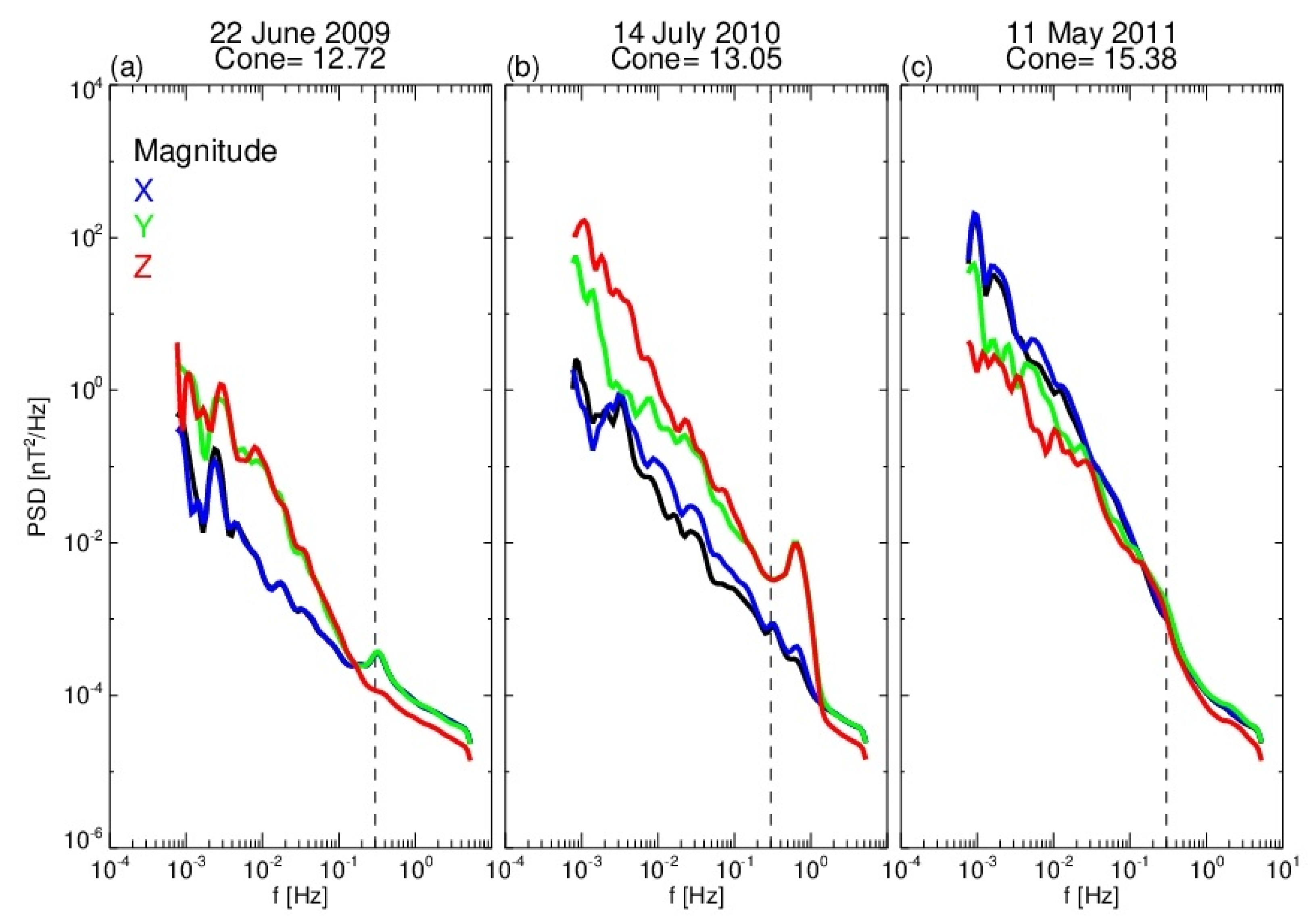
3.1. Characteristic of PSD for Radial IMF Events

We use the wavelet technique [25] and calculate the magnetic power spectrum densities (PSDs) in 1-h windows. The calculations start 4 h prior to the identified interval and end 4 h after the trailing edge of the radial IMF interval without any overlap. The PSDs calculated prior to and after the interval of the radial field will be used later for comparisons, and thus we discarded PSDs from windows adjacent to the radial IMF interval because the radial field may still influence surrounding regions. In total, 2393 intervals in 419 radial IMF events and 2514 intervals in both adjacent regions are used for PSD calculations.

The first issue of interest is the behavior of slopes in the radial IMF events. For this study, we first removed PSDs that do not allow us to determine the slope well. Figure 2 displays three typical PSD profiles in the radial IMF events. Figure 2a shows the PSD profile with a peak at f = 0.33 Hz that belongs to the satellite spin rate, and it becomes more pronounced when the PSD power is low. We also frequently observe a peak at other frequencies (Figure 2b) connected to possible wave structures in the solar wind. Since the waves or coherent structures can influence the PSD slopes [26], the periods with these two types of PSD are excluded from slope analysis. The last type is shown in Figure 2c. PSDs computed from three components and magnitude are very similar, but no clear break can be identified. We suppose that that there are two possible reasons leading to this PSD shape: (1) The break exists at a higher frequency than we analyze, or (2) the signal amplitude is close to the background noise [27]. Such events are also not included in our statistics. The same criteria are also applied to the adjacent regions. Finally, 332 (415) intervals in radial IMF events (in adjacent regions) were selected for estimation of the fluctuation power and PSD slopes.

Figure 3b shows all PSD profiles in the selected intervals of radial IMF, and Figure 3a,c show the profiles in the regions before and after the radial IMF events, respectively. In contrast to Figure 2, where the PSDs of the magnetic field components are shown, we use the trace PSDs in Figure 3 and also in all following studies. We can note that almost all PSD profiles in the radial IMF intervals (Figure 3b) exhibit a lower power than PSDs in adjacent regions; the power at a given frequency is up to two orders of magnitude lower than that reported in several previous studies, e.g., [28], under various IMF orientations. This feature was also observed by Pi et al. [7] in the time series of the magnetic field data, and we can conclude that the low fluctuation amplitude is a typical feature of the radial IMF events. The green lines in Figure 3 stand for the PSD of noise determined by [27]. We can see that, especially at higher frequencies, our PSDs often touch the noise limit.

Our study concentrates on the quantitative assessment of the fluctuation power and PSD slopes in MHD and kinetic ranges of frequencies. The slopes were calculated by a linear fitting in a fixed interval of frequencies (0.003–0.03 Hz) for the MHD range and in a fixed interval of power (0.001–0.01 nT²/Hz) for the kinetic range. These margins are shown in Figure 3 as the blue dashed lines. The power in the MHD range is represented by the median value of the powers in the same frequency range as used for slope calculation. However, it is almost impossible to find a suitable frequency range in the kinetic range, and thus this study uses a fixed power range to replace the fixed frequency range. As it can be seen in Figure 3, this choice minimizes the effect of the spacecraft spin and magnetometer noise on the resulting parameters. In order to further reduce the influence from the noise, we remove the points that have a low signal-to-noise ratio (less than 5). This margin is plotted in Figure 3 by the green dashed line, and all points below the green dashed line are excluded from slope computations. Additionally, we also do not calculate the slope if the number of points for fitting is lower than eight (a factor of two in the frequency range). For the power in the kinetic range, we use the Taylor hypothesis that connects the spacecraft frame frequency with spatial dimensions of the observed structures and select the inertial-length frequency [29] as the reference frequency (the red points in Figure 3). Since the breakpoint between the MHD and kinetic ranges is close to the sum of the inertial length and proton thermal gyroradius [29], the inertial length frequency is located close to the break but is clearly in the kinetic range. The power representing the kinetic range is then calculated as a difference between values of PSDs of the signal and noise corresponding to the inertial-length frequency.

Figure 4 shows the distributions of slopes in different regions in the MHD (left panel) and kinetic (right panel) ranges of frequencies. The black-filled area represents the distribution in the radial IMF intervals, and the green/red lines stand for the adjacent regions prior to/after the intervals of a radial IMF. The slopes in the MHD range have a median value of −1.5 ± 0.2 for the radial IMF intervals, but this value is rather −1.6 ± 0.2 in both adjacent regions with other orientations. We can conclude that the median slope is a little shallower in the intervals of the radial IMF, but the broadness of the slope distributions is similar in all regions. The median slope in the kinetic range is steeper in the radial IMF events with a median value of −2.5 ± 0.5, whereas the medians are −2.2 ± 0.5 in the adjacent regions. Taking into account the broadness of distributions, this difference is small, but the figure shows the clear shift of a whole distribution. Moreover, the distribution of slopes corresponding to the intervals of the radial IMF is also a little narrower.

Figure 5 uses the same format as Figure 4 and shows the distributions of powers in the MHD and kinetic ranges. In both ranges, we can see the difference between radial IMF events and the adjacent regions. As it has already been noted, the fluctuation of power in the intervals of the radial IMF is lower than that in the adjacent regions. In the MHD range, the median value is 3.38 nT²/Hz, whereas it is 5.84 and 6.46 nT²/Hz in the adjacent regions. A similar difference is observed in the kinetic range: 0.0010 nT²/Hz in intervals of the radial IMF and 0.0024 and 0.0027 nT²/Hz in the adjacent regions. Note that although the average power in the adjacent regions is higher than that in the radial IMF events, it is still lower than in the regular solar wind, e.g., [28].

3.2. Temperature Anisotropy and β

This particular statistical study is motivated by the last panel in Figure 1 showing that the temperature anisotropy (T_ANI = T_P⊥/T_P‖) is larger than 1 in this individual radial IMF interval, whereas it is typically lower than 1 (around 0.8, e.g., [30]) in the solar wind. This anisotropy arises because the plasma can move freely along the magnetic field line and due to the ion beam effect [31]. Bale et al. [32] have shown that the different T_ANI values can lead to different spectra in the kinetic range and Lion et al. [26] pointed out that the coherent structures corresponding to a spacecraft frame frequency near ion cyclotron frequency can influence the slopes in the kinetic range. Thus, it is important to understand the T_ANI distribution in the radial IMF events. Figure 6 shows the histogram of temperature anisotropies in radial IMF events and adjacent regions in the same format as Figure 4. It is clear that T_ANI in radial IMF intervals is in a systematic manner larger than that in the adjacent regions, and its median value is even close to unity (0.976).

The larger parallel than perpendicular temperature acts in the early stage of the solar wind expansion from the Sun. The IMF is preferentially radial there, but the solar wind expands in the perpendicular direction and the expansion thus decreases the perpendicular temperature preferentially. One could expect that this effect would also act in our radial events, but Figure 6 reveals an opposite trend. Since the temperature anisotropy is regulated by the excitation of different kinds of waves, we checked the distribution of temperature anisotropy and parallel proton beta, ${\beta }_{\Vert P}$ (the ratio of the parallel proton thermal and magnetic pressures). Figure 7 shows a distribution of these quantities in the radial IMF events (Figure 7a) and intervals prior to (Figure 7b) and after (Figure 7c) the events. The selected periods are the same as those in Figure 5. The curved lines denote the thresholds of the mirror, proton cyclotron, parallel firehose, and oblique firehose instabilities. These thresholds are described in [33]; the governing equation is:

$$T_{ANI}=\frac{T_{p\perp }}{T_{p\Vert }}=1+\frac{a}{{\left({\beta }_{\Vert p}-{\beta }_0\right)}^b},$$

(1)

where $a$, b, ${\beta }_0$ are the fitted parameters summarized in Table 1 of [33]. Those parameters are calculated in the ranges 0.01 < ${\beta }_{\Vert P}$ < 100 and 0.1 < $T_{ANI}$ < 10 and associated with the maximum growth rate in [33]. The color scale represents the normalized occurrence rate in $T_{ANI}$-${\beta }_{\Vert P}$ bins. This rate is calculated as a ratio of the number of observations in each particular bin and the total number of observations. The figure shows that the distributions in adjacent regions are similar to those already published, e.g., [33] and exhibit a peak at larger ${\beta }_{\Vert P}$ and $T_{ANI}$ lower than 1 (Figure 7b,c). On the other hand, a peak along $T_{ANI}$ = 1 that is evenly distributed along the ${\beta }_{\Vert P}$ axis is observed in the radial IMF events.

In order to show these features more clearly, Figure 7d presents the difference between the distributions in the radial IMF events and adjacent regions. The difference (Del) is calculated by Equation (2):

$$Del=V_r-\frac{\left(V_{be}+V_{af}\right)}{2}\times \frac{1}{De{l}_{max}},$$

(2)

where $V_r$ is the occurrence rate within a particular $T_{ANI}$ and ${\beta }_{\Vert P}$ bin for the radial IMF events, $V_{be}$ and $V_{af}$ are the occurrence rates in the same ranges of $T_{ANI}$ and ${\beta }_{\Vert P}$ for the intervals prior to and after the radial events, and $De{l}_{max}$ is the maximum absolute value for all $T_{ANI}$ and ${\beta }_{\Vert P}$ bins. The figure clearly indicates that there are more observations with low ${\beta }_{\Vert P}$ and slightly positive $T_{ANI}$ and less observations with high ${\beta }_{\Vert P}$ and negative $T_{ANI}$ in the radial events.

3.3. Observations of Waves

The $T_{ANI}$-${\beta }_{\Vert P}$ plot in the last chapter suggests that the proton cyclotron instability can be more often triggered in the radial IMF events than in the adjacent regions. For this reason, we carried out a preliminary wave analysis. We have visually inspected the PSDs of magnetic field components and found that 699 of 2393 radial events exhibit a clear peak (see Figure 2b as an example). However, a similar feature was sparsely found in the adjacent regions (56/2514), and it implies that there are more wave-like structures in the radial IMF events. For a more precise analysis, we calculated the coherence and phase differences between B_Y and B_Z by the wavelet coherence technique [34] and used the following steps to select the intervals with possible wave activity:

• Each PSD was fitted with a linear fit in a log-log scale.
• The fitted profile was subtracted from the original PSD (compensated PSD).
• The frequency range below 0.01 Hz was omitted.
• The maximum of compensated PSD was found.
• Only PSDs with a peak exceeding 0.5 were selected.
• The remaining PSDs were checked on the coherence of B_Y and B_Z (perpendicular components).
• Only PSDs exhibiting coherence above 0.8 in more than 10% of the observed points (10 min) were accepted.
• Finally, 485 intervals with wave structures (from 2393 intervals) were selected for further analysis.

Figure 8 shows the distribution of the selected intervals in the phase difference and frequency plane. The plane is divided into four quadrants, and the numbers at the center of the figure represent the number of intervals in each quadrant. Previous studies showed that the low-frequency waves (f < 0.1 Hz) would be the Alfvén waves dominated by the left-hand polarization, e.g., [35]. The high-frequency range (f > 0.1 Hz) would be also predominantly occupied by the left-hand polarized electromagnetic cyclotron waves with a small percentage of right-hand waves [36]. Nevertheless, our results for radial IMF events show some differences. The low-frequency waves (0.01–0.1 Hz) are mostly left-hand polarized (negative phase difference), but the high-frequency waves (f > 0.1 Hz) have no preferential polarization. The right-hand polarized cases are observed even slightly more frequently than the left-hand waves.

4. Discussion

Previous studies show that the power and slopes of magnetic field PSDs depend on the cone angle in the MHD and kinetic ranges, e.g., [12,13]. A small cone angle results in the low power in the MHD range and steeper slopes in both MHD and kinetic ranges. In Figure 3 and Figure 5, we can see that the fluctuation power in the radial IMF events is lower than that in the adjacent regions for both frequency ranges (the mean value dropped from around 6.0 to 3.4 nT²/Hz in the MHD range and from 0.0026 to 0.0010 nT²/Hz in the kinetic range). Although the limitation of the cone angle can naturally decrease the fluctuation amplitude of the magnetic field, the fluctuation amplitude decrease is a common behavior of all solar wind parameters under the radial IMF [7]. Therefore, there should be other reasons to reduce the fluctuation amplitude. Figure 9 presents how the power varies with the cone angle. The power in the MHD range increases with the cone angle in all regions; however, the power and cone angle are independent in the kinetic range. In the adjacent regions, the power trend is consistent with [12]. They found around a two orders of magnitude difference between small and large cone angles in the MHD range. Since the cone angle range is small in the radial IMF set, the power difference at small and large cone angles is not so big, but the trend is similar to that in the adjacent regions. The power in the kinetic range is independent of the cone angle at all analyzed regions. In agreement with already published results, we can conclude that the magnetic field is more stable under quasi-radial IMF conditions. However, the radial IMF events might be not as “quiet” as we think. The observation limitations could cause the low fluctuation amplitude. Zank et al. [37] developed a nearly incompressible MHD turbulence theory. In the frame of this theory, a possible interpretation of our finding is the simultaneous coexistence of two-dimensional (2D) and slab fluctuations. Two-dimensional turbulence is characterized by a wavevector perpendicular to the background magnetic field, B₀, whereas slab fluctuations are characterized by a wavevector parallel to B₀. These extreme situations are very rare in solar wind, and the power of these fluctuations is distributed across a finite range of angles around the 2D and slab limits. The magnetic field, B, can be expressed as:

$$B=B_0+B^{\infty }+B^{*},$$

(3)

where $B^{\infty }$ describes the prevailing 2D component of the magnetic field fluctuations, and $B^{*}$ represents higher-order corrections that include slab, quasi-2D, and compressible fluctuations. The 2D component dominates the fluctuation amplitude, and the ratio between the 2D and slab is approximately $\left|B^{\infty }\right|:\left|B^{*}\right|=80:20$. If IMF is oriented radially, we scan the fluctuations along $B$, and thus we observe predominantly $B^{*}$, and information on 2D fluctuations is limited. Without the full information of the 2D fluctuation, the power determined in the long-lasting radial IMF events cannot adequately represent the “real” fluctuation amplitude, and the use of the radial IMF events as a “quiet” solar wind condition can be misleading.

The slope in the kinetic range is slightly steeper, whereas the slope in the MHD range is less steep than those in the adjacent regions (see Figure 4; the mean slop is −1.5/−1.6 in the radial IMF events/adjacent regions for the MHD range and −2.5/−2.2 for the kinetic range). Figure 10 shows the relation between the cone angle and the slopes. In the region prior to the events, the result is consistent with previous studies that the slopes decrease when the cone angle turns to the radial direction, although the difference found in our data set is nearly negligible. However, similar trends are absent in the radial IMF events and in the region after the events. For our long-lasting radial IMF events, the median slopes in the MHD range are almost independent on the cone angle, with a possible decreasing trend when the cone angle increases. The median slopes in the cone angle bins range from −1.6 to −1.4.

Duan et al. [13] presented the first results from the Parker Solar Probe observations near the Sun. The slope dramatically steepens for the cone angle between 30° to 0° in the kinetic range being near −7 for purely parallel conditions. A similar result is also predicted by Chen et al. [38]. In our study of the long-lasting radial IMF events, no noticeable trend with the cone angle was found in all regions, and the steepest observed slope is just around −4 (see Figure 4). We found that T_ANI is large in the radial IMF events (see Figure 7), and Bale et al. [32] shows that the large T_ANI can flatten the slope in the kinetic range. It can be the reason for the observed flattening of slopes. Nevertheless, we should note that the magnetometer noise can affect the determination of slopes in the kinetic range [39], and thus the real slope can be steeper.

In a short summary, the power of the magnetic fluctuations in the long-lasting radial IMF intervals shows a similar behavior as in other regions, but the behavior of slopes is different. The slopes are slightly flatter in the MHD range but steeper in the kinetic range for radial IMF events. The variations are smaller than those in the adjacent regions and exhibit an opposite trend than the adjacent regions and previous studies. This conflict can be caused by the special structure of a radial IMF, which leads to a different development of turbulence. The primary reason for the anisotropy is that the energy transfer rate depends on θk_B, the angle between the wave vector and the mean magnetic field [40]. It leads to the anisotropies of the PSD power level and slope. The wave vector anisotropy is expected around $k_{\parallel }~k_{\perp }^{\raisebox{1ex}{$2$}\!\left/ \!\raisebox{-1ex}{$3$}\right.}$ or $k_{\parallel }~k_{\perp }^{\raisebox{1ex}{$1$}\!\left/ \!\raisebox{-1ex}{$2$}\right.}$ [41,42], where $k_{\parallel }$ is the wave vector parallel and $k_{\perp }$ is the wave vector perpendicular to the B₀ direction. This anisotropy is connected with the solar wind expansion. In the simulation results of [42], the difference between spectral indices in the strongly and weakly expanded solar wind events is reported. There is no clear difference between them for the perpendicular magnetic field fluctuations, but the power spectrum is less steep in the strongly expanded case for the parallel fluctuations (from −5/3 for strongly expanded to −3/2 for weakly expanded). The long-lasting radial IMF events would be regarded as an over-expanded region, e.g., [7]. Therefore, this effect can result in slightly flattened PSD in the MHD range in a comparison with the adjacent regions and observed steepening with increasing cone angle (see Figure 9a–c).

Figure 6 shows that T_ANI approaches 1 in the radial IMF event. Before the discussions about the T_ANI, we should point out that the uncertainties of perpendicular and parallel temperature determination change with the angle between the sampling and magnetic field directions [43]. When this angle approaches 0°, the perpendicular uncertainty increases, and the parallel one decreases. These observation limitations lead to a large uncertainty of T_ANI in the radial IMF events of around 50%, whereas it would be around 23% for a Parker spiral orientation. As we mentioned, T_ANI could be caused by the perpendicular solar wind expansion during its propagation through interplanetary space. The radial IMF events are usually observed in the solar wind speed decreasing areas such as rarefaction regions, but the solar wind also expands in the radial direction in these regions. Therefore, both perpendicular and parallel temperatures could decrease there due to the expansion. On the other hand, the isotropic temperature may be caused by the solar wind heating in the direction perpendicular to the main field. Gary & Borovsky [44] pointed out that the cyclotron resonance between kinetic Alfvén wave (KAW) and protons can increase the proton temperature in the perpendicular direction. Moreover, KAW stochastic heating can also affect the perpendicular temperature [45], and recent observational results support these mechanisms [46,47,48]. For example, Telloni et al. [49] show that the high-frequency Alfvén waves heat protons in a direction perpendicular to the magnetic field and increase the temperature anisotropy. Moreover, the same observational study shows that the heating in the perpendicular direction is more significant when ${\beta }_{\Vert P}$ is small, and this is the case of the radial IMF events. One more factor in controlling the perpendicular heating reported in the same paper is the angle between the proton and alpha particle speeds. The perpendicular heating effect is more substantial when the alpha particle speed is oriented along the solar wind proton speed, as in the case of the radial IMF events.

One more interesting issue is the polarization of waves at frequencies higher than 0.1 Hz. In the recent years, numerous studies have shown the behavior of these waves in the solar wind. These waves are transverse and propagate in the direction parallel or antiparallel to the background magnetic field. According to the background magnetic field, they can be left- or right-hand polarized in the spacecraft frame, but they are usually dominated by the left-hand polarization [36]. However, our results are different. In the solar wind, the parallel firehouse instability can generate magnetosonic waves that propagate toward the Sun, and the proton cyclotron instability can generate ion cyclotron waves propagating away from the Sun [50,51]. Both these two wave types show the left-hand polarization in the spacecraft frame. The right-hand polarized waves can be the oblique Alfvén-ion cyclotron waves, but oblique fast-mode/whistler waves are not excluded [52]. However, our results show no apparent difference between the left- and right-hand cases in the event number. A previous study [53] reveals that the occurrence rate of electromagnetic cyclotron waves is around 1.8%, but it is much higher in the small-sample statistical result of radial IMF events, around 5% (we found 485 cases containing wave structures among 2393 intervals). This result is consistent with the observation [54,55] that these waves are preferentially detected in the rarefaction region and when the IMF points to the radial direction. The proton beam that can lead to an instability of the proton distribution function is one of possible mechanisms [56]. The study [53] presents monthly changes of left-hand electromagnetic cyclotron wave percentage. In some months, the percentages can be lower than 0.5. Bruno and Telloni [57] show the preferred polarization in different parts of the rarefaction region and indicated that the polarization changes. He et al. [58,59] show that the magnetic helicity changes with the cone angle. Those results imply that the electromagnetic cyclotron waves can be without a preferred polarization in solar wind structures such as the radial IMF events.

In Figure 7, the distribution in the $T_{ANI}$-${\beta }_{\Vert P}$ plane shows that the ion cyclotron wave can be more frequently generated in the radial IMF events. However, the sources of the right-hand polarized waves seem to be complicated. Figure 11 shows the histogram of the frequency normalized to the ion cyclotron frequency, average solar wind bulk speed, and mean B_X of the intervals with different polarizations (red for left-hand and blue for right-hand polarization). The right-hand polarization cases have a broad distribution of the normalized frequency and prefer a slower solar wind than the left-hand cases (Figure 11a,b). Right-hand polarized waves often arise when B_X points to the Sun, and left-hand polarizations have opposite preferences. The distribution of right-hand polarized waves shows a double peak structure with the normalized frequency. The two peaks appear at around 0.2 and 1 times of the ion cyclotron frequency, but the left-hand distribution only has a single peak around 0.5 times of the ion cyclotron frequency. The previous statistical studies [53,54] revealed that the left-hand polarized waves prefer a higher median frequency and solar wind speed than the right-hand one. It may be related with the peak of the right-hand distribution at 1. However, the other peak of the right-hand polarized waves implies that the right-hand polarized waves may be composed of more than one type of waves. The wave properties in the radial IMF events require more precise studies in the future.

5. Conclusions

In this paper, the unusual behavior of magnetic fluctuations in the long-lasting radial IMF events is presented. A total of 419 long-lasting (more than 4 h) radial interplanetary magnetic field (IMF) events were found in 15 years of Wind spacecraft observations. The power spectral density (PSD), coherence, and phase differences are calculated by wavelet analysis for each 1-h interval in the radial IMF events and its adjacent regions. The results are summarized as follows:

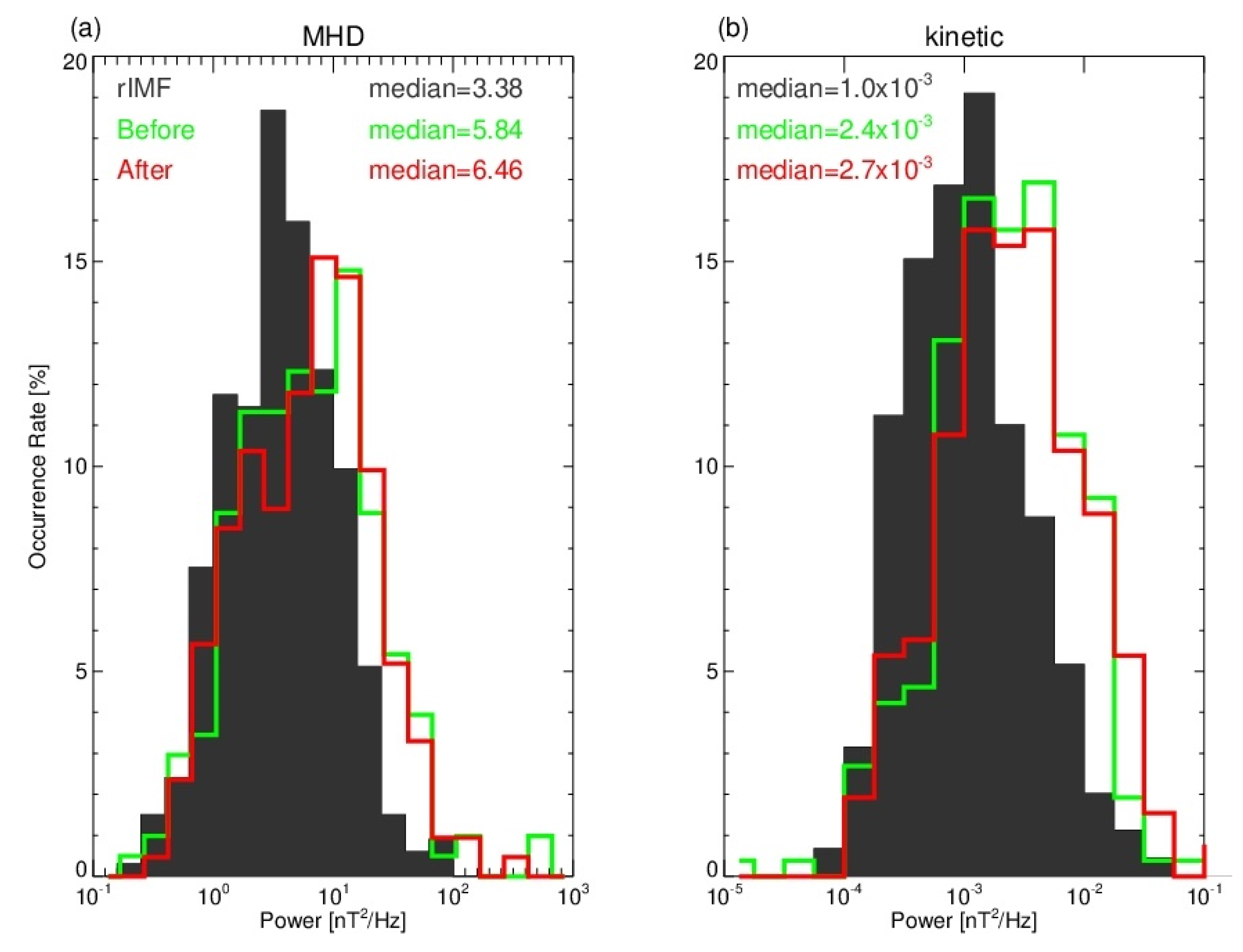
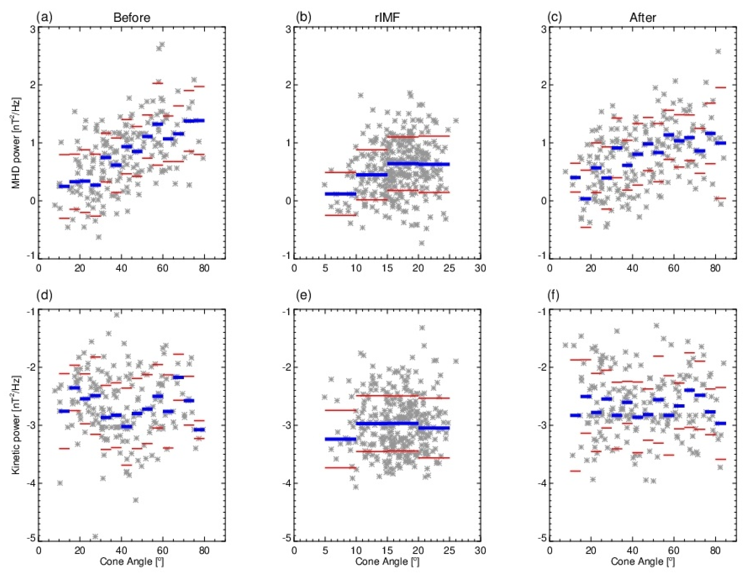
• The fluctuation powers are low in the radial IMF events in both MHD and kinetic ranges, which is consistent with the previous observational results showing that the power increases with increasing cone angle (from 6.0 to 3.4 nT²/Hz in the MHD range and 0.0026 to 0.0010 nT²/Hz in the kinetic range).
• Although the observed fluctuation power is low, the above conclusion can be misleading due to observation limitations. The dominant 2D component of the magnetic fluctuation is hard to observe because the sampling direction is aligned with the mean magnetic field.
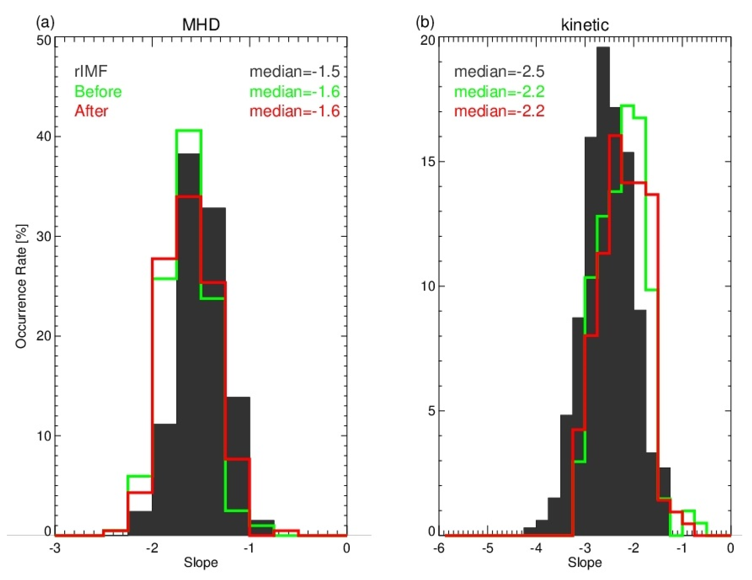
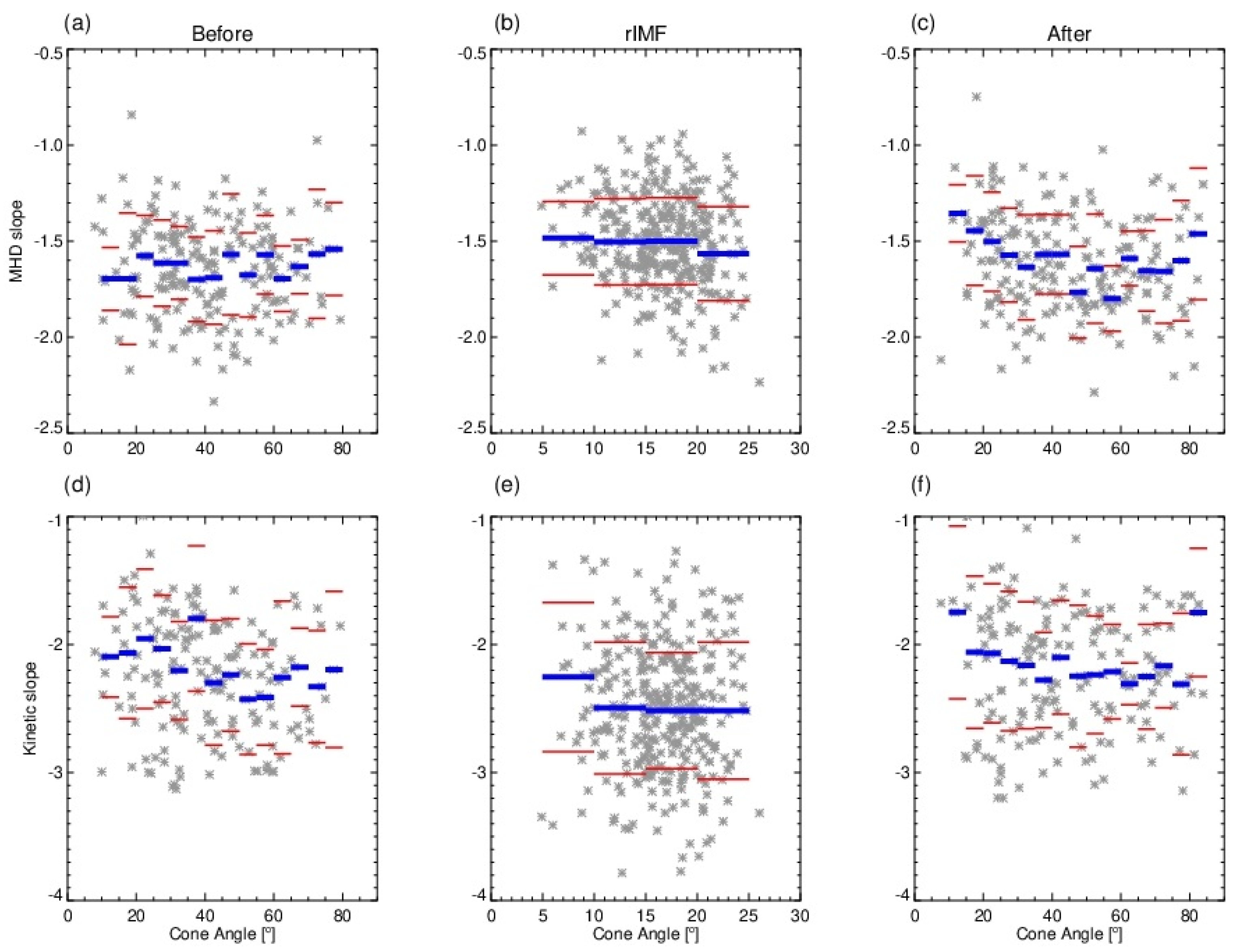
• Compared with the adjacent regions, the median slope of the PSD is slightly steeper (−2.5) in the kinetic range and less steep in the MHD range (−1.5), but the formerly reported dependence of the PSD slope on the cone angle is missing in the radial IMF events. It might be related to the development of turbulence in long-lasting radial IMF intervals. An over-expansion forming these intervals can result in a flatter slope of the solar wind magnetic fluctuations.
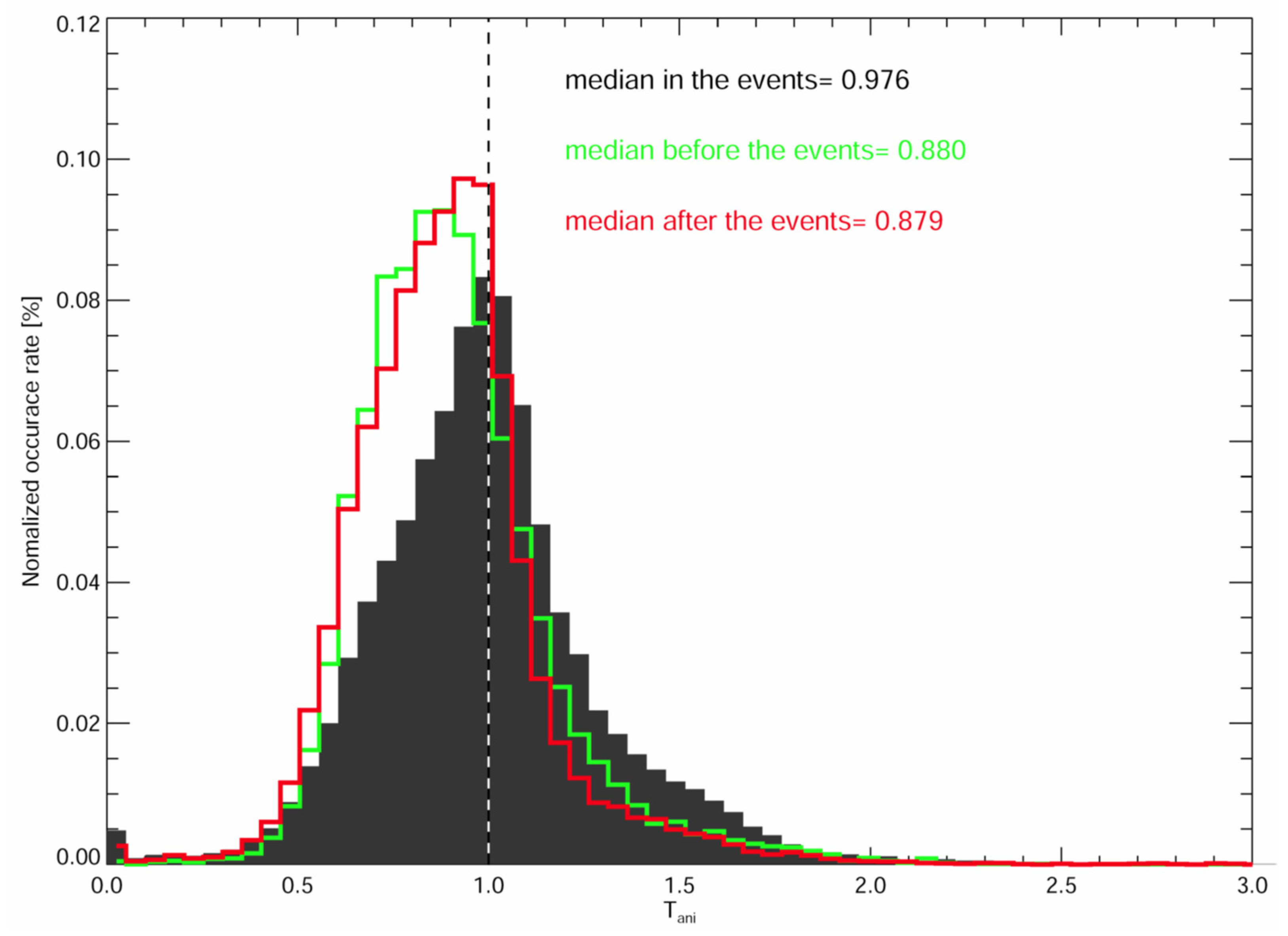
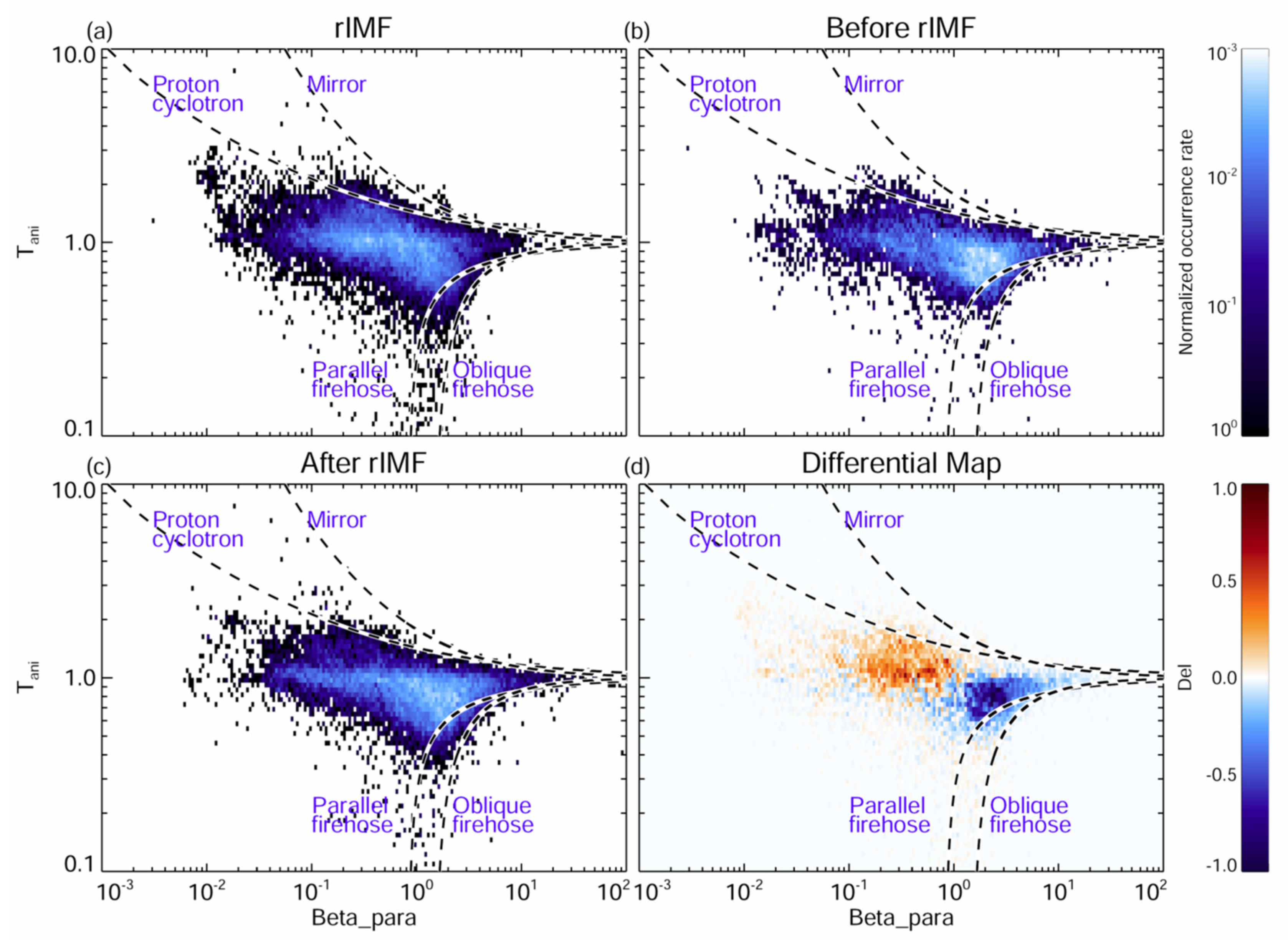
• The temperature is more isotropic in the radial IMF events. We suggest that radial expansion in these events is larger than that in a typical Parker-spiral structure, and it leads to the enhancement of parallel cooling. On the other hand, stochastic processes can more efficiently heat protons in perpendicular direction in a low ${\beta }_{\Vert P}$ plasma with a small angle between the alpha particle and proton speeds.
• The occurrence rate of wavy structures in the frequency range above 0.01 Hz is higher in radial IMF events. This result is consistent with the distribution of T_ANI-${\beta }_{\Vert P}$, showing that the proton cyclotron instability has a higher chance to be excited in the radial IMF events.
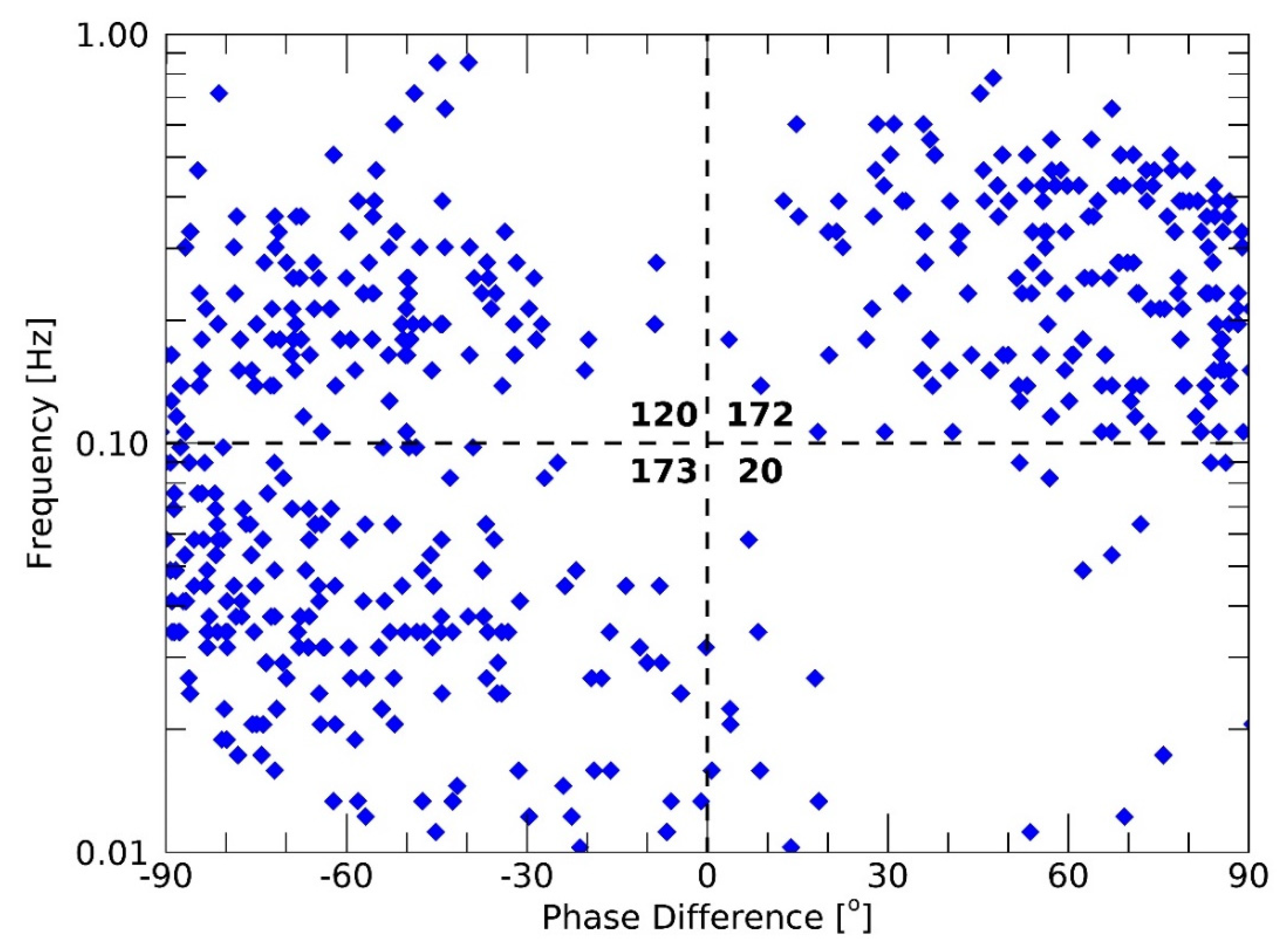
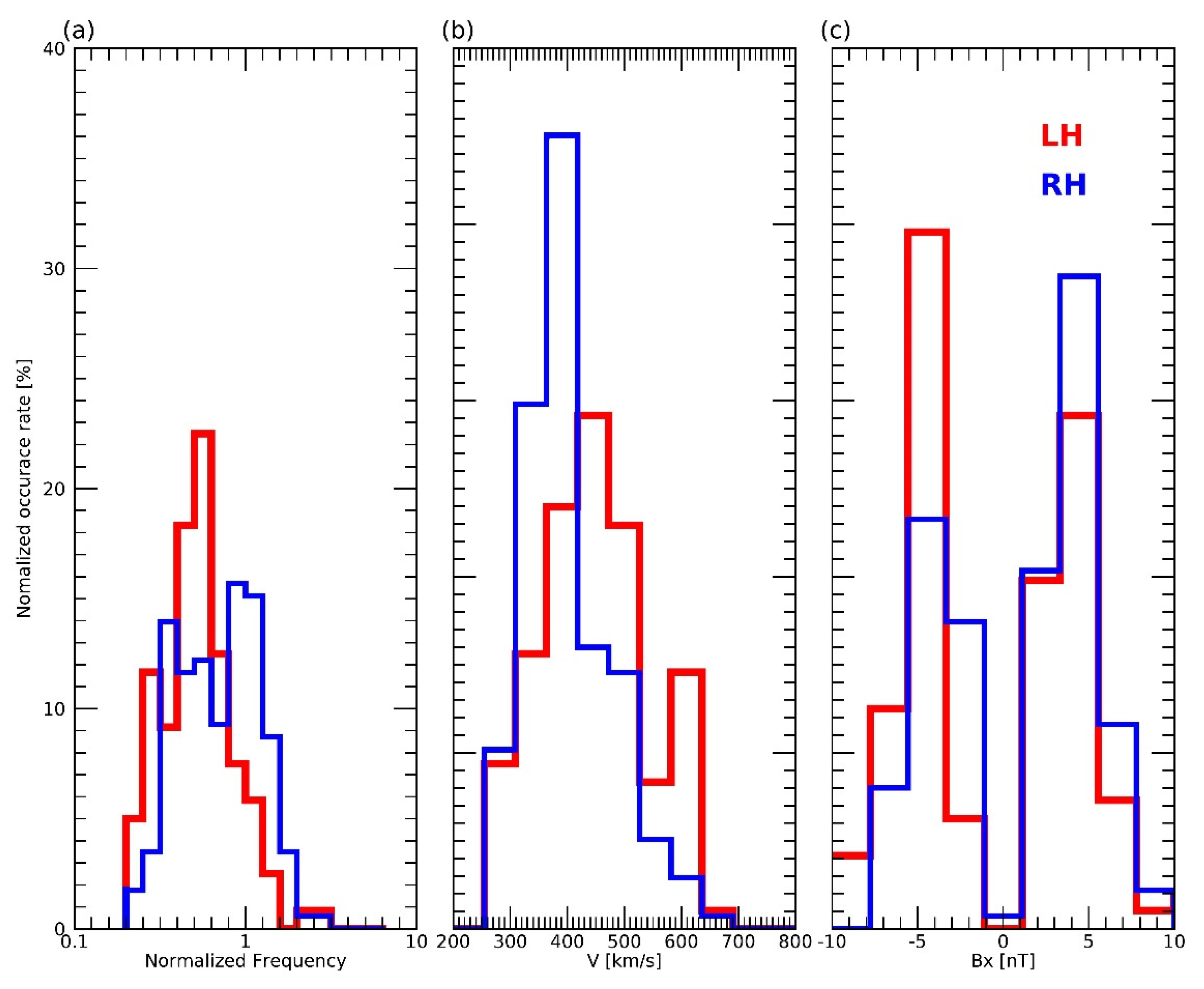
• We did not find a clear preferred wave polarization in the radial IMF events in a frequency range from 0.1 to 1 Hz, but the right-hand polarized waves are observed slightly more frequently than the left-hand ones.

References

1. Shue, J.H.; Chao, J.K.; Fu, H.C.; Russell, C.T.; Song, P.; Khurana, K.K.; Singer, H.J. A new functional form to study the solar wind control of the magnetpause size and shape. J. Geophys. Res. 1997, 102, 9497–9511. [Google Scholar] [CrossRef]
2. Sibeck, D.G.; Lin, R.-Q. Size and shape of the distant magnetotail. J. Geophys. Res. Space Phys. 2014, 119, 1028–1043. [Google Scholar] [CrossRef]
3. Dungey, J.W. Interplanetary magnetic field and the auroral zone. Phys. Rev. Lett. 1961, 6, 47–48. [Google Scholar] [CrossRef]
4. Dungey, J.W. The Structure of the Ionosphere, or Adventures in Velocity Space. In Geophysics: The Earth’s Environment; Dewitt, C., Hieblot, J., Lebeau, A., Eds.; Gordon and Breach: New York, NY, USA, 1963; pp. 503–550. [Google Scholar]
5. Bier, E.A.; Owusu, N.; Engebretson, M.J.; Posch, J.L.; Lessard, M.R.; Pilipenko, V.A. Investigating the IMF cone angle control of Pc3-4 pulsations observed on the ground. J. Geophys. Res. Space Phys. 2014, 119, 1797–1813. [Google Scholar] [CrossRef]
6. Pi, G.; Němeček, Z.; Šafránková, J.; Grygorov, K.; Shue, J.-H. Formation of the dayside magnetopause and its boundary layers under the radial IMF. J. Geophys. Res. Space Phys. 2018, 123, 3533–3547. [Google Scholar] [CrossRef] [Green Version]
7. Pi, G.; Shue, J.-H.; Chao, J.-K.; Němeček, Z.; Šafránková, J.; Lin, C.-H. A reexamination of long-duration radial IMF events. J. Geophys. Res. Space Phys. 2014, 119, 7005–7011. [Google Scholar] [CrossRef]
8. Gosling, J.T.; Skoug, R.M. On the origin of radial magnetic fields in the heliosphere. J. Geophys. Res. 2002, 107, 1327. [Google Scholar] [CrossRef]
9. Schwadron, N.A. An Explanation for Strongly Underwound Magnetic Field in Co-rotating Rarefaction Regions and its Relationship to Footpoint Motion on the the Sun. Geophys. Res. Lett. 2002, 29, 8-1–8-4. [Google Scholar] [CrossRef] [Green Version]
10. Klein, K.G.; Howes, G.G.; TenBarge, J.M.; Podesta, J.J. Physical interpretation of the angle-dependent magnetic helicity spectrum in the solar wind: The nature of turbulent fluctuations near the proton cyroradius scale. APJ 2014, 785, 138. [Google Scholar] [CrossRef] [Green Version]
11. Horbury, T.S.; Forman, M.; Oughton, S. Anisotropic Scaling of Magnetohydrodynamic Turbulence. Phys. Rev. Lett. 2008, 101, 175005. [Google Scholar] [CrossRef] [Green Version]
12. Podesta, J.J. Dependence of solar-wind power spectra on the direction of the local mean magnetic field. APJ 2009, 698, 986–999. [Google Scholar] [CrossRef]
13. Duan, D.; He, J.; Bowen, T.A.; Woodham, L.D.; Wang, T.; Chen, C.H.K.; Mallet, A.; Bale, S.D. Anisotropy of Solar Wind Turbulence in the Inner Heliosphere at Kinetic Scales: PSP Observations. ApJL 2021, 915, L8. [Google Scholar] [CrossRef]
14. Wicks, R.T.; Horbury, T.S.; Chen, C.H.K.; Schekochihin, A.A. Power and spectral index anisotropy of the entire inertial range of turbulence in the fast solar wind. Mon. Not. R. Astron. Soc. Lett. 2010, 407, L31. [Google Scholar] [CrossRef] [Green Version]
15. He, J.; Tu, C.; Marsch, E.; Bourouaine, S.; Pei, Z. Radial evolution of the wavevector anisotrooy of solar wind turbulence between 0.3 and 1 AU. APJ 2013, 773, 72. [Google Scholar] [CrossRef] [Green Version]
16. Wang, X.; Tu, C.; He, J.; Marsch, E.; Wang, L. The influence of intermittency on the spectral anisotropy of solar wind turbulence. ApJL 2015, 810, L21. [Google Scholar] [CrossRef]
17. Wu, H.; Tu, C.; Wang, X.; He, J.; Yang, L.; Wang, L. Isotropic Scaling Features Measured Locally in the Solar Wind Turbulence with Stationary Background Field. APJ 2020, 892, 138. [Google Scholar] [CrossRef]
18. Zank, G.P.; Nakanotani, M.; Zhao, L.-L.; Adhikari, L.; Telloni, D. Spectral Anisotropy in 2D plus Slab Magnetohydrodynamic Turbulence in the Solar Wind and Upper Corona. APJ 2020, 900, 115. [Google Scholar] [CrossRef]
19. Oughton, S.; Matthaeus, W.H. Critical Balance and the Physics of Magnetohydrodynamic Turbulence. Astrophys. J. 2020, 897, 37. [Google Scholar] [CrossRef]
20. Suvorova, A.V.; Shue, J.-H.; Dmitriev, A.V.; Sibeck, D.G.; McFadden, J.P.; Hasegawa, H.; Ackerson, K.; Jelínek, K.; Šafránková, J.; Němeček, Z. Magnetopause expansions for quasi-radial interplanetary magnetic field: THEMIS and Geotail observations. J. Geophys. Res. 2010, 115, A10216. [Google Scholar] [CrossRef] [Green Version]
21. Suvorova, A.V.; Dmitriev, A.V. Magnetopause inflation under radial IMF: Comparison of models. Earth Space Sci. 2015, 2, 107–114. [Google Scholar] [CrossRef]
22. Telloni, D.; Carbone, F.; Bruno, R.; Sorriso-Valvo, L.; Zank, G.P.; Adhikari, L.; Hunana, P. No Evidence for Critical Balance in Field-aligned Alfvenic Solar Wind Turbulence. Astrophys. J. 2019, 887, 160. [Google Scholar] [CrossRef]
23. Ogilvie, K.W.; Chornay, D.J.; Fritzenreiter, R.J.; Hunsaker, F.; Keller, J.; Lobell, J.; Miller, G.; Scudder, J.D.; Sittler, E.C., Jr.; Torbert, R.B.; et al. SWE, A comprehensive plasma instrument for the Wind spacecraft. Space Sci. Rev. 1995, 71, 55–77. [Google Scholar] [CrossRef]
24. Lepping, R.P.; Acuna, M.H.; Burlaga, L.F.; Farrall, W.M.; Slavin, J.A.; Schatten, K.H.; Mariani, F.; Ness, N.F.; Neubauer, F.M.; Whang, Y.C.; et al. The WIND magnetic field investigation. Space Sci. Rev. 1995, 71, 207–229. [Google Scholar] [CrossRef]
25. Torrence, C.; Compo, G.P. A practical guide to wavelet analysis. Bull. Am. Meteorol. Soc. 1998, 79, 61–78. [Google Scholar] [CrossRef] [Green Version]
26. Lion, S.; Alexandrova, O.; Zaslavsky, A. Coherent Events and Spectral Shape at Ion Kinetic Scales in the Fast Solar Wind Turbulence. Astrophys. J. 2016, 824, 47. [Google Scholar] [CrossRef] [Green Version]
27. Woodham, L.D.; Wicks, R.T.; Verscharen, D.; Owen, C.J. The Role of Proton Cyclotron Resonance as a Dissipation Mechanism in Solar Wind Turbulence: A Statistical Study at Ion-kinetic Scales. APJ 2018, 856, 49. [Google Scholar] [CrossRef]
28. Pi, G.; Pitňa, A.; Němeček, Z.; Šafránková, J.; Shue, J.-H.; Yang, Y.-H. Long- and Short-Term Evolutions of Magnetic Field Fluctuations in High-Speed Streams. Sol. Phys. 2020, 295, 84. [Google Scholar] [CrossRef]
29. Safrankova, J.; Nemecek, Z.; Nemec, F.; Prech, L.; Chen, C.H.K.; Zastenker, G.N. Power Spectral Density of Fluctuations of Bulk and Thermal Speeds in the Solar Wind. Astrophys. J. 2016, 825, 121. [Google Scholar] [CrossRef] [Green Version]
30. Mullan, D.J.; Smith, C.W. Solar wind statistics at 1 AU: Alfven speed and plasma beta. Sol. Phys. 2006, 234, 325–338. [Google Scholar] [CrossRef]
31. Němeček, Z.; Šafránková, J.; Němec, F.; Ďurovcová, T.; Pitňa, A.; Alterman, B.L.; Voitenko, Y.M.; Pavlů, J.; Stevens, M.L. Spectra of Temperature Fluctuations in the Solar Wind. Atmosphere 2021, 12, 1277. [Google Scholar] [CrossRef]
32. Bale, S.D.; Kasper, J.C.; Howes, G.G.; Quataert, E.; Salem, C.; Sundkvist, D. Magnetic Fluctuation Power Near Proton Temperature Anisotropy Instability Thresholds in the Solar Wind. Phys. Rev. Lett. 2009, 103, 211101. [Google Scholar] [CrossRef] [PubMed] [Green Version]
33. Hellinger, P.; Trávníček, P.; Kasper, J.C.; Lazarus, A.J. Solar wind proton temperature anisotropy: Linear theory and WIND/SWE observations. Geophys. Res. Lett. 2006, 33, L09101. [Google Scholar] [CrossRef] [Green Version]
34. Torrence, C.; Webster, P.J. Interdecadal changes in the ENSO-monsoon system. J. Clim. 1999, 12, 2679–2690. [Google Scholar] [CrossRef] [Green Version]
35. Bruno, R.; Carbone, V. The solar wind as a turbulence laboratory. Lining Rev. Sol. Phys. 2013, 10, 2. [Google Scholar] [CrossRef] [Green Version]
36. Jian, L.K.; Wei, H.Y.; Russell, C.T.; Luhmann, J.G.; Klecker, B.; Omidi, N.; Isenberg, P.A.; Goldstein, M.L.; Figueroa-Viñas, A.; Blanco-Cano, X. Electromagnetic waves near the proton cyclotron frequency: STEREO observations. Astrophys. J. 2014, 786, 123. [Google Scholar] [CrossRef]
37. Zank, G.P.; Adhikari, L.; Shiota, P.H.D.; Bruno, R.; Telloni, D. Theory and Transport of Nearly Incompressible Magnetohydrodynamic Turbulence. APJ 2017, 835, 147. [Google Scholar] [CrossRef]
38. Chen, C.H.K.; Wicks, R.T.; Horbury, T.S.; Schekochihin, A.A. Interpreting power anisotropy measurements in plasma turbulence. ApJL 2010, 711, L79. [Google Scholar] [CrossRef] [Green Version]
39. Pitňa, A.; Šafránková, J.; Němeček, Z.; Franci, L.; Pi, G. A Novel Method for Estimating the Intrinsic Magnetic Field Spectrum of Kinetic-Range Turbulence. Atmosphere 2021, 12, 1547. [Google Scholar] [CrossRef]
40. Goldreich, P.; Sridhar, S. Toward a theory of interstellar turbulence II. Strong Alfvénic turbulence. APJ 1995, 438, 763. [Google Scholar] [CrossRef]
41. Boldyrev, S. Spectrum of Magnetohydrodynamic Turbulence. Phys. Rev. Lett. 2006, 96, 115002. [Google Scholar] [CrossRef] [Green Version]
42. Verdini, A.; Grappin, R.; Alexandrova, O.; Franci, L.; Landi, S.; Matteini, L.; Papini, E. Three-dimensional local anisotropy of velocity fluctuations in the solar wind. Mon. Not. R. Astron. Soc. 2019, 486, 3006–3018. [Google Scholar] [CrossRef]
43. Woodham, L.D.; Wicks, R.T.; Verscharen, D.; TenBarge, J.M.; Howes, G.G. Dependence of Solar Wind Proton Temperature on the Polarization Properties of Alfvenic Fluctuations at Ion-kinetic Scales. Astrophys. J. 2021, 912, 101. [Google Scholar] [CrossRef]
44. Gary, S.P.; Borovsky, J.E. Alfvén-cyclotron fluctuations: Linear Vlasov theory. J. Geophys. Res. Space Phys. 2004, 109, A6. [Google Scholar] [CrossRef]
45. Chandran BD, G.; Li, B.; Rogers, B.N.; Quataert, E.; Germaschewski, K. Perpendicular Ion Heating by Low-frequency Alfvén-wave Turbulence in the Solar Wind. APJ 2010, 720, 503C. [Google Scholar] [CrossRef]
46. Zhao, G.Q.; Feng, H.Q.; Wu, D.J.; Huang, J.; Zhao, Y.; Liu, Q.; Tian, Z.J. Dependence of Ion Temperatures on Alpha–Proton Differential Flow Vector and Heating Mechanisms in the Solar Wind. ApJL 2020, 889, L14. [Google Scholar] [CrossRef]
47. Zhao, G.Q.; Lin, Y.; Wang, X.Y.; Wu, D.J.; Feng, H.Q.; Liu, Q.; Zhao, A.; Li, H.B. Observational Evidence for Solar Wind Proton Heating by Ion-Scale Turbulence. Geophys. Res. Lett. 2020, 47, 18. [Google Scholar] [CrossRef]
48. Zhao, G.Q.; Lin, Y.; Wang, X.Y.; Feng, H.Q.; Wu, D.J.; Li, H.B.; Zhao, A.; Liu, Q. Magnetic Helicity Signature and Its Role in Regulating Magnetic Energy Spectra and Proton Temperatures in the Solar Wind. APJ 2021, 906, 123. [Google Scholar] [CrossRef]
49. Telloni, D.; Carbone, F.; Bruno, R.; Zank, G.P.; Sorriso-Valvo, L.; Mancuso, S. Ion Cyclotron Waves in Field-aligned Solar Wind Turbulence. Astrophys. J. Lett. 2019, 885, L5. [Google Scholar] [CrossRef]
50. Podesta, J.J.; Gary, S.P. Magnetic helicity spectrum of solar wind fluctuations as a function of the angle with respect to the local mean magnetic field. APJ 2011, 734, 15. [Google Scholar] [CrossRef]
51. Jian, L.K.; Russell, C.T.; Luhmann, J.G.; Anderson, B.J.; Boardsen, S.A.; Strangeway, R.J.; Cowee, M.M.; Wennmacher, A. Observations of ion cyclotron waves in the solar wind near 0.3 AU. J. Geophys. Res. Space Phys. 2010, 115. [Google Scholar] [CrossRef] [Green Version]
52. He, J.S.; Tu, C.Y.; Marsch, E.; Yao, S. Do Oblique Alfven/Ion-Cyclotron or Fast-Mode/Whistler Waves Dominate the Dissipation of Solar Wind Turbulence near the Proton Inertial Length? Astrophys. J. Lett. 2012, 745, L8. [Google Scholar] [CrossRef]
53. Zhao, G.Q.; Feng, H.Q.; Wu, D.J.; Liu, Q.; Zhao, U.; Zhao, A.; Huang, J. Statistical study of low-frequency electromagnetic cyclotron waves in the solar wind at 1 AU. J. Geophys. Res. Space Phys. 2018, 123, 1715–1730. [Google Scholar] [CrossRef]
54. Zhao, G.Q.; Chu, Y.H.; Lin, P.H.; Yang, Y.-H.; Feng, H.Q.; Wu, D.J.; Liu, Q. Low-frequency electromagnetic cyclotron waves in and around magnetic clouds: STEREO observations during 2007–2013. J. Geophys. Res. Space Phys. 2017, 122, 4879–4894. [Google Scholar] [CrossRef]
55. Jian, L.K.; Moya, P.S.; Vinas, A.F.; Stevens, M. Electromagnetic Cyclotron Waves in the Solar Wind: Wind Observation and Wave Dispersion Analysis. AIP Conf. Proc. 2016, 1720, 040007. [Google Scholar] [CrossRef]
56. Wicks, R.T.; Alexander, R.L.; Stevens, M.; Wilson, L.B.; Moya, P.S.; Vinas, A.; Jian, L.K.; Roberts, D.A.; O’Modhrain, S.; Gilbert, J.A.; et al. A Proton-Cyclotron Wave Storm Generated by Unstable Proton Distribution Functions in the Solar Wind. Astrophys. J. 2016, 819, 6. [Google Scholar] [CrossRef] [Green Version]
57. Bruno, R.; Telloni, D. Spectral Analysis of Magnetic Fluctuations at Proton Scales from Fast to Slow Solar Wind. Astrophys. J. Lett. 2015, 811, L17. [Google Scholar] [CrossRef] [Green Version]
58. He, J.S.; Marsch, E.; Tu, C.; Yao, S.; Tian, H. Possible Evidence of Alfven-Cyclotron Waves in the Angle Distribution of Magnetic Helicity of Solar Wind Turbulence. Astrophys. J. 2011, 731, 85. [Google Scholar] [CrossRef]
59. He, J.S.; Tu, C.Y.; Marsch, E.; Yao, S. Reproduction of the Observed Two-Component Magnetic Helicity in Solar Wind Turbulence by a Superposition of Parallel and Oblique Alfven Waves. Astrophys. J. 2012, 749, 86. [Google Scholar] [CrossRef] [Green Version]
Figure 1. An example of a long-lasting radial IMF event. From top to bottom: (a) | B x | B , (b) magnitude and three components of the magnetic field in GSE coordinates (blue for BX, green for BY, red for BZ), (c) solar wind speed, (d) Y- and Z-components of solar wind speed, (e) proton number density, (f) proton thermal speed, (g) perpendicular (blue) and parallel (red) thermal speed, and (h) temperature anisotropy.
Atmosphere 13 00173 g001
Figure 2. Three typical types of PSD profiles of magnitude and three components of the magnetic field (black for magnitude, blue for BX, green for BY, red for BZ) in the radial IMF events. The dashed lines denote the spin rate of the Wind spacecraft. (a) data from 22 June 2009, (b) data from 14 July 2010, (c) data from 11 May 2011.
Atmosphere 13 00173 g002
Figure 3. PSD profiles computed in all selected 1-h intervals: (a) before the radial IMF events, (b) in the radial IMF events, and (c) after the radial IMF events. The black dotted lines mark the intervals for calculations of the PSD slopes in the MHD (vertical) and kinetic (horizontal) scales. The solid and dashed green lines represent the noise floor and 5 times of the noise floor, respectively. The red points denote the inertial length frequency for each interval.
Atmosphere 13 00173 g003
Figure 4. Histograms of the PSD slopes in (a) the MHD and (b) kinetic ranges. The black regions illustrate the results in the radial IMF events. Green (before)/red (after) lines represent the results from the adjacent regions. Median values are marked in corresponding panels.
Atmosphere 13 00173 g004
Figure 5. Histograms of the PSD powers in (a) the MHD and (b) kinetic ranges. The format and colors are the same as in Figure 4.
Atmosphere 13 00173 g005
Figure 6. Histograms of TANI of all observations. The format and colors are the same as in Figure 4.
Atmosphere 13 00173 g006
Figure 7. Distribution of T A N I - β P (a) in the radial IMF events, (b) before, and (c) after the events. The dashed curved lines denote the thresholds of Mirror, Proton cyclotron, Parallel firehose, and Oblique firehose instabilities. (d) represents the difference between the distribution in the radial IMF events and the mean values of adjacent regions (Del).
Atmosphere 13 00173 g007
Figure 8. Distributions of the phase difference and frequency for the selected wavy intervals. The numbers at the center of the figure denote the number of intervals in each quadrant.
Atmosphere 13 00173 g008
Figure 9. Scatter plots of the PSD power as a function of the cone angle (a) in the region before the radial IMF events, (b) in the radial IMF events, and (c) after the events in the MHD ranges and the same plots (d) in the region before the radial IMF events, (e) in the radial IMF events, and (f) after the events in the kinetic ranges. The blue bars represent the median value in each 5° bin, and the red bars denote the standard deviation of each bin.
Atmosphere 13 00173 g009
Figure 10. Scatter plots of the PSD slopes as a function of the cone angle with the same format as Figure 9: (a) in the region before the radial IMF events, (b) in the radial IMF events, and (c) after the events in the MHD ranges and the same plots (d) in the region before the radial IMF events, (e) in the radial IMF events, and (f) after the events in the kinetic ranges.
Atmosphere 13 00173 g010
Figure 11. Histograms of the corresponding conditions of the wavy intervals: (a) the frequency normalized by the corresponding ion cyclotron frequency, (b) solar wind speed, and (c) BX component. The blue lines represent the results from the right-hand polarized intervals, and red lines represent the results from the left-hand polarized intervals.
Atmosphere 13 00173 g011
Publisher’s Note: MDPI stays neutral with regard to jurisdictional claims in published maps and institutional affiliations.