Article

Changing Emissions Results in Changed PM2.5 Composition and Health Impacts

1
Institute for a Sustainable Environment, Clarkson University, Potsdam, NY 13699, USA
2
Department of Public Health Sciences, University of Rochester School of Medicine and Dentistry, Rochster, NY 14642, USA
3
Envair/Aerochem, Placitas, NM 87043, USA
*
Author to whom correspondence should be addressed.
Atmosphere 2022, 13(2), 193; https://doi.org/10.3390/atmos13020193
Submission received: 3 January 2022 / Revised: 18 January 2022 / Accepted: 19 January 2022 / Published: 25 January 2022
(This article belongs to the Special Issue Urban Air Chemistry in Changing Times)

Abstract

:
In the period of 2005 to 2016, multiple air pollution control regulations have entered into effect in the United States at both the Federal and state level. In addition, economic changes have also occurred primarily in the electricity generation sector that substantially changed the emissions from this sector. This combination of policy implementations and economics has led to substantial reductions in PM2.5, its major constituents, and source specific PM2.5 concentrations across the New York State, particularly those of sulfate, nitrate, and primary organic carbon. However, secondary organic carbon and spark-ignition vehicular emission contributions have increased. Related studies of changes in health outcomes, the excess rates of emergency department visits and hospitalizations for a variety of cardiovascular and respiratory diseases and respiratory infections have increased per unit mass of PM2.5. It appears that the increased toxicity per unit mass was due to the reduction in low toxicity constituents such that the remaining mass had greater impacts on public health.

1. Introduction

Air pollution and its environmental response have been a major stimulus for the study of urban air chemistry. In the absence of changes in meteorology and chemical loss processes, changes in air chemistry have taken place largely from the regulation to the control of emissions. Since the 1950s, the knowledge of the physico-chemical characteristics of tropospheric aerosols has greatly expanded. Urban aerosols have seen reductions in mass concentration and major changes in chemical processing and composition, which are reflected in changes in human health measures.
The United States has made substantial progress in reducing ambient air pollution since the passage of the Clean Air Act Amendments of 1970. Thus, by 2005, there was a decrease from an approximate national mean PM2.5 concentration of 23.28 µg/m3 measured between 1 April 1979 and 30 June 1980 in the Inhalable Particulate Network [1] to a national mean value of 12.63 µg/m3 [2]. However, there were still many areas out of compliance with the National Ambient Air Quality Standard for PM2.5. Thus, additional policies have been implemented in the period of 2005 to 2016 that have specified an improvement in liquid fuel quality, increase fuel economy for light-duty, spark-ignition vehicles, controls on emissions from heavy-duty diesel vehicles and non-road vehicles, and reductions in emissions from electricity generating units (EGUs), particularly coal-fired power plants. During this same period, there have been significant economic drivers that have resulted in a substantial change in fuel use in EGUs because of the low cost of fracked natural gas.
To assess these changes in emissions, air quality, and health indicators in the New York State, several studies were conducted to assess trends in pollutant emissions and concentrations [3,4,5,6], identify the major sources and their trends [6,7,8], and examine the changes in the associations of PM2.5 and source-specific PM2.5 hospitalizations and emergency department visits for cardiovascular disease [9,10]. This paper provides a review of these findings with a focus on the urban sites across New York where both mass concentrations and chemical speciation of PM2.5 measurements were made and presents their implications for the next steps needed to reduce particulate pollution and improve public health.

2. Materials and Methods

The data utilized in the previously noted studies were all obtained from the U.S. Environmental Protection Agency (USEPA). They are accessible directly from the USEPA (https://aqs.epa.gov/aqsweb/airdata/download_files.html#Raw (accessed on 12 January 2016)) or the Federal Land Manager Environmental Database (http://views.cira.colostate.edu/fed/Auth/Login.aspx?ReturnUrl=%2ffed%2fQueryWizard%2fDefault.aspx (accessed on 12 January 2016)). During the period of 2005 to 2016, there were up to 63 monitoring sites across New York State operated by the New York State Department of Environmental Conservation. The focus in this review will be on six urban sites (Buffalo, Rochester, Albany and 3 sites in New York City) since these urban areas represent the bulk of the population of the state and provided the health data that supported the epidemiological studies. Data on PM2.5 measured using Federal Equivalence Method (FEM) technology and PM2.5 compositional data obtained from the Chemical Speciation Network [11] were used in the original work. The health data for these studies were obtained from the New York State Department of Health Statewide Planning and Research Cooperative System (SPARCS) database.
The data analyses on the temporal variations in concentrations were conducted using a variety of data analytic packages in R [12] particularly ‘openair’ [13]. Details of these analyses are provided by Squizzato et al. [3] and Masiol et al. [8]. The source apportionments were performed using the EPA-PMF V5.014 as described by Squizzato et al. [7]. The health assessments were all conducted using a time-stratified, case-crossover design and conditional logistic regression analyses [14,15]. Details of the selection of subjects and the control of confounding variables, such as temperature and relative humidity, are provided in the previously published epidemiological reports for PM2.5 and cardiovascular diseases [9], respiratory infections [16], and respiratory diseases [17]. The same methods were employed to assess the impacts of source-specific PM2.5 on adverse health outcomes as reported for cardiovascular diseases [10], respiratory infections [18], and respiratory diseases [19].

3. Results

3.1. Policies and Economic Drivers Affecting PM2.5 Concentrations

3.1.1. Electricity Generating Units

A number of reduction strategies have been implemented to reduce emissions from electricity generating units (EGUs) that was a major contributor to the formation of secondary inorganic PM2.5 species. The 1998 NOx SIP (State Implementation Plan) Call [20] and the 2003 NOx Budget Trading Program [21] were promulgated in 1998 to reduce ozone concentrations in the eastern United States by reducing precursor emissions and their transport. The SIP Call did not directly regulate specific sources, but rather required states to undertake programs to reduce NOx emissions during the ozone season. The trading program established a cap-and-trade program to facilitate states to be able to meet their emission reduction goals. To further reduce interstate transport of NOx and SO2, the USEPA promulgated the Clean Air Interstate Rule (CAIR) in 2005. The CAIR initiated additional emissions trading programs to reduce annual emissions of SO2 and NOx as well as specifically reducing NOx during the ozone season. The CAIR was challenged in court for lack of legislative authorization and, in 2008, the CAIR was upheld. However, EPA was required to replace the CAIR with a new set of regulations. The new regulations were the Cross State Air Pollution Rule (CSAPR) [22,23,24]. In addition to the direct regulatory pressures on EGU emissions of SO2 and NOx, there were the resolutions of a series of suits by the U.S. government against power companies who had made significant changes to the production facilities, such as U.S. vs. American Electric Power [25], which required the addition of emission controls on many old EGUs.
However, the recession of 2007–2009 reduced the demand for electricity at the same time that low-cost fracked natural gas was becoming plentiful. The low price of gas changed the economics of electricity generation such that it was more effective to build and operate new combined cycle gas turbines than to restart the coal-fired power plants after the demand for electricity returned to the pre-recession level [3].

3.1.2. Vehicles and Liquid Fuel Quality

A second major contributor to the urban PM2.5 chemistry are the emissions from vehicles and transportation. In the U.S., for example, the monthly production of vehicles that ranged from 750 thousand to 1.5 million was added to the existing fleet, most of which reside in an urban environment. This category of “reactants” historically involves sulfur and nitrogen oxide emissions and volatile organic compounds (VOC) as well traces of metals. Major changes in these emissions have occurred in response to the extensive regulations that have been implemented since the 1970s.
Emission limits for both light-duty [26] and heavy-duty on-road vehicles [27] were set as well as limits on sulfur in on-road vehicular fuels. Light-duty vehicles (max. 8500 lb Gross Vehicle Weight Rating (GVWR)) include passenger vehicles, light-duty trucks, and medium-duty passenger vehicles (max. 10,000 lb GVWR). These regulations were to be phased in from 2004 to 2009. For new passenger cars (LDVs) and LLDTs, Tier 2 standards phase-in begun in 2004, with full implementation in the 2007 model year. For HLDTs and MDPVs, the Tier 2 standards were phased in beginning in 2008, with full compliance in 2009.
For heavy-duty engines and related fuel, PM emission standards took effect for all new heavy-duty vehicles sold after 1 July 2007. To meet the PM emission limits required the use of catalytic regenerative particulate traps. The NOx standard was phased-in for diesel engines between 2007 and 2010. The phase-in was defined on a percent-of-sales basis: 50% from 2007 to 2009 and 100% in 2010. To avoid poisoning the catalyst in the traps, it was necessary to reduce the sulfur content in on-road diesel fuel to ultralow sulfur (<15 ppm S). As of 1 October 2006, 80% of all on-road diesel fuel was to be ultralow S with 100% attained by 1 January 2010 [28].
In 2004, Tier 4 emission standards were promulgated to control air pollution from nonroad diesel engines and fuels [29]. They were to be phased-in over the period of 2008–2015. To enable sulfur-sensitive control technologies in Tier 4 engines, including catalytic particulate traps and NOx adsorbers, EPA mandated reductions in sulfur content in nonroad diesel fuels. Effective June 2007 nonroad, locomotive and marine (NRLM) diesel fuels had to have <500 ppm S; effective June 2010 nonroad fuel had to be ultralow S; and locomotive and marine fuels had to be ultralow S by June 2012. Ultimately, this federal requirement was relaxed to 1 January 2014 [29]. However, beginning 1 July 2012, New York required that all distillate oils, including No. 2 oil sold within the state for any purpose, be ultralow sulfur.
The space heating of large buildings in New York City was typically by burning residual (No. 6) oil because of its low cost. Because of the difficulties in distributing No. 6 given it needs to be heated to flow, No. 2 oil was mixed 50/50 with No. 6 to produce No. 4 oil. The use of No. 6 oil was allowed through the issue of 3-year-period permits by the New York City government. Beginning in 2011, New York City no longer issued new permits for No. 6 oil use, so by 2015, only No. 4 or cleaner oils could be used. However, No. 4 oil could still contain 1500 ppm S [30]. A 16% reduction in PM2.5 between 2008 and 2014 was attributed to reductions in emissions from building heating because of the switch to cleaner fuels [31].
Based on the timing of the implementation of these regulations and economic drivers, changes in the period of 2005 to 2016 were divided into three subperiods: Before (2005–2007), which represents time prior to or early in the implementation of the regulations; During (2008 to 2013), when many of the regulations were being implemented; and After (2014 to 2016), when most of the required changes were made. Differences in concentrations, source contributions, and health effects were assessed for each subperiod. The differences appeared in net reductions of SO2, NOx, VOCs, and PM (including composition) emissions.

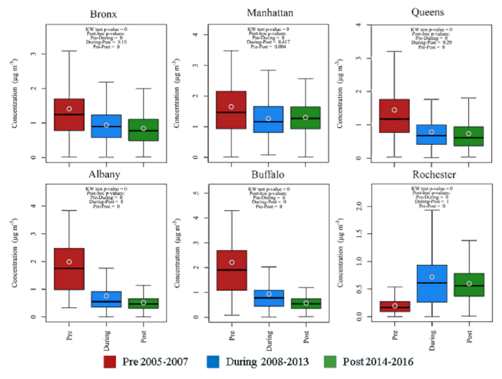
3.2. Trends in Concentrations

Squizzato et al. [3] examined the monotonic trends in PM2.5 concentrations from 2005 to 2016 using Thiel–Sen slope [31,32]. The slope and related confidence intervals for the whole year and seasonal trends are provided in Table 1. There were substantial reductions in PM2.5 at all six New York State sites in the range of 3 to 4% per year.
The trends on the gaseous criteria pollutants (CO, NOx, SO2, and O3) were also presented in detail in Squizzato et al. [3]. Significant reductions in CO, NOx, and SO2 as well as peak summer O3 values were observed across the New York State. However, increases in annual average O3 concentrations were observed. Spring maxima O3 values did not change and autumn and winter O3 values increased [3].

3.3. Source Apportionments

Various changes in the operation of the Chemical Speciation Network presented challenges to the PMF analyses [11]. The largest issue was the change in the sampling and analysis procedures for organic (OC) and elemental carbon (EC) that occurred between 2007 and 2009 [11]. The change in OC/EC protocol for NIOSH to IMPROVE-A [33]. The IMPROVE-A analyses provided carbon fraction data that had been previously shown to be useful in separating gasoline from diesel vehicle contributions (e.g., [34,35]) that is lacking in the NIOSH results. Thus, separate PMF analyses were required pre and post this change for the source apportionments. However, there was a good degree of agreement in the identified sources between these two time periods. The results of the analyses are summarized in Table 2 separated into the average results in pre-OC/EC change and the post-OC/EC change periods. Squizzato et al. [7] reported that six sources were identified at all the urban sites. These sources were: secondary sulfate (SS), secondary nitrate (SN), gasoline emissions (GAS), diesel emissions (DIE), biomass burning (BB), and road dust (RD). Road salt was found in each of the upstate sites (Buffalo, Rochester, and Albany) where the roads need to be cleared of the substantial winter snowfalls. In New York City (NYC), three additional sources were resolved: fresh sea salt (FSS), aged sea salt (AGS), and residual oil (RO). In Buffalo, an unknown “industrial” source was found. The major sources were secondary sulfate, secondary nitrate, gasoline vehicles, and diesel vehicles. The temporal patterns (seasonal, monthly, and day of week) were discussed in detail by Squizzato et al. [11], with sulfate peaks in the summer while nitrate peaks in the winter. Diesel contributions are higher on weekdays than on weekend days. Road salt is a winter source as is residual oil and fresh sea salt driven by coastal storms that are more common in January to March. Aged sea salt is higher in summer when there is greater photochemical activity leading to the formation of gaseous acids that can react with the sea salt and displace the chlorine. Biomass burning in NYC had summer peaks that are likely the result of wildfire aerosols transported into the area and summertime outdoor cooking. However, it is a winter source in the upstate cities where recreational wood combustion is common [36,37], and in some households, there is home heating with wood combustion. The OP-rich factor is one that has been commonly observed in the analysis of composition data that include the IMPROVE OC/EC carbon fractions. It has been suggested to represent a combination of aged secondary organic aerosols (SOAs) and associated secondary sulfate [35,36,38] and possibly long-range transported wildfires.

3.4. Trends in Source Contributions

To examine the differences among the three defined periods (before, during, and after), the distributions of the source contributions were compared among them. Figure 1, Figure 2, Figure 3 and Figure 4 show the distributions for SS, SN, GAS, and DIE. A Kruskal–Wallis ANOVA test on ranks [39] was used to compare the distributions across the three periods and the results are provided in the figures.
In general, the source-specific concentrations for all of the sources were the highest during the before period with decreasing trends in the following periods. GAS is a notable exception where there is an increasing trend across the three periods with a substantial increase in the after period. Large decreases in SS and SN with the increases in GAS and a relatively smaller decline in diesel means that vehicular-emissions-related PM2.5 represented an increasing fraction of the remaining PM2.5 concentrations.
To understand the rise in GAS in the during and after periods, it is necessary to examine the changes in both light-duty engine technology and fuel composition. The 1975 Energy Policy Conservation Act added Title V, Improving Automotive Efficiency, to the Motor Vehicle Information and Cost Savings Act and established Corporate Average Fuel Economy (CAFE) standards for passenger cars and light-duty trucks (LDT). From 1990 onward to 2011, the standard was set at 27.5 mpg for cars. The standard for trucks increased from 20.2 to 23.5 mpg by 2010. Effective in 2011, a reformulation of the CAFE standards set standards depending on vehicle size and were setting more stringent requirements. During the 2008 to 2011 period, manufacturers could meet the existing standards or the new reformulated standards. At the beginning of our study, the standard light-duty engine used port-fuel injection (PFI). However, gasoline-direct inject (GDI) was being to be developed to provide improved fuel efficiency. Table 3 shows the penetration of GDI technology into the new car market. Thus, in the after period, there was a substantial penetration of GDI vehicles into the on-road fleet. However, Zhao et al. [40] used a potential aerosol mass (PAM) oxidation flow reactor during chassis dynamometer testing using the cold-start unified cycle (UC) to examine the formation of secondary organic aerosols (SOAs) in diluted exhausts from both PFI and DGI equipped vehicles. They found for Tier 2 vehicles that GDI vehicle exhaust resulted in higher production of SOAs than PFI vehicles. This higher SOA production modifies the chemistry of the organic fraction of PM2.5 that is formed from contemporary vehicle emissions.
In addition, another change occurred in the formulation of gasoline between 2011 and 2014 driven by the Mobile Source Air Toxics (MSAT2) benzene standard that required reductions in the benzene concentrations to 0.62 volume percent by 2016 from a 2000 average of 1.15 volume percent. The 2016 average was 0.51 volume percent. To compensate for the loss of antiknock performance due to the reduced benzene concentration, the concentrations of intermediate volatility organic compounds (IVOCs) were increased. IVOCs include polycyclic aromatic hydrocarbons and aliphatic compounds with carbon chain lengths of 12 to 22 [41]. These IVOC compounds are much more effective in producing SOAs compared to single-ring aromatic compounds. To assess the relationship between the GAS concentrations and the secondary organic carbon (SOC) values, SOC concentrations were estimated from the organic and elemental carbon data using the method of Lim and Turpin [42] and the lowest 10th percentile values of the OC/EC ratios to define the primary OC/EC relationship. The GAS values had the highest correlations with the SOC values at all six sites. The moderate r2 values were: Buffalo 0.504; Rochester 0.533; Albany 0.423; Manhattan 0.303; Bronx 0.548; and Queens 0.533.
The combined reductions in EGU emissions and changes in vehicle emissions because of fuel composition changes have modified the chemical composition of PM2.5 resulting in reduced sulfate, nitrate and ammonium, and replaced by secondary organic carbon. The OC fraction changed between 2005 and 2016 in response to the increased secondary component formation and reduced primary OC emissions. Further changes in PM2.5 can be expected in mass or number concentration and composition with the evolution of internal combustion engines and the market penetration of electric vehicles.

3.5. Trends in Health Outcomes

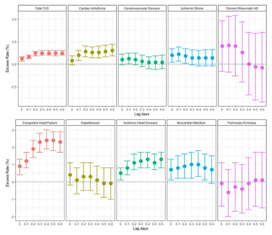
3.5.1. Cardiovascular Diseases

The excess rates of hospitalizations for cardiovascular diseases (CVD) (Total CVD, cardia arrhythmias, cerebrovascular disease, ischemic stroke, chronic rheumatic heart disease, congestive heart failure, hypertension, ischemic heart disease, myocardial infarctions, and pulmonary embolisms) were estimated for the whole 12-year period and for the 3 subperiods. These results are based on a total of 1,922,918 cardiovascular hospital admissions during the study period. Of these admissions, 82.1% were in New York City (Manhattan, Queens, Bronx), with the largest proportion in Manhattan (29.6%; n = 568,933) and the smallest proportion in Albany (4.2%; n = 81,250). These whole period results for lag days from 0 to 0–6 are presented in Figure 5. There are statistically significant associations for Total CVD, arrhythmias, ischemic stroke, congestive heart failure, ischemic heart disease, and myocardial infarctions. In addition to the analysis across all of New York, individual site results were calculated, and the meta-analysis performed yielded very similar results showing a substantial homogeneity of responses among the six locations.
The excess rates (%) associated with interquartile range (IQR) increases in PM2.5 for the cardiovascular diseases among the three periods are shown in Figure 6 for the outcomes that had significant values over the whole period. There are several significant shifts in the lag-day patterns as well as the magnitude of the effects. There is a particular increase in the excess rates per IQR for Total CVD, ischemic heart disease, and myocardial infarctions.
To further explore the changes in inferred toxicity per IQR PM2.5 mass among the periods, source-specific PM2.5 associations with hospitalizations for the various cardiovascular outcomes were determined [10]. Because the samples are collected only every 3rd or every 6th day, lag days here can only represent the average of day 0 and day 3 (0–3) or days 0, 3, and 6 (0–6). Figure 7 shows the results for selected source types where statistically significant excess rates were observed.
GAS was the source type most strongly associated with arrythmias and less strongly with ischemic stroke and myocardial infarctions and GAS was the only source that increased significantly in the after period. DIE also was strongly associated as are RO and RD, and at most sites they did not change in concentration across the study period. There were no observable associations with SS and SN was only associated with myocardial infarctions. BB had a significant protective effect on ischemic heart disease. The reason for such an association is unclear except that it may reflect personal behaviors that keep individuals away from exposure sources.

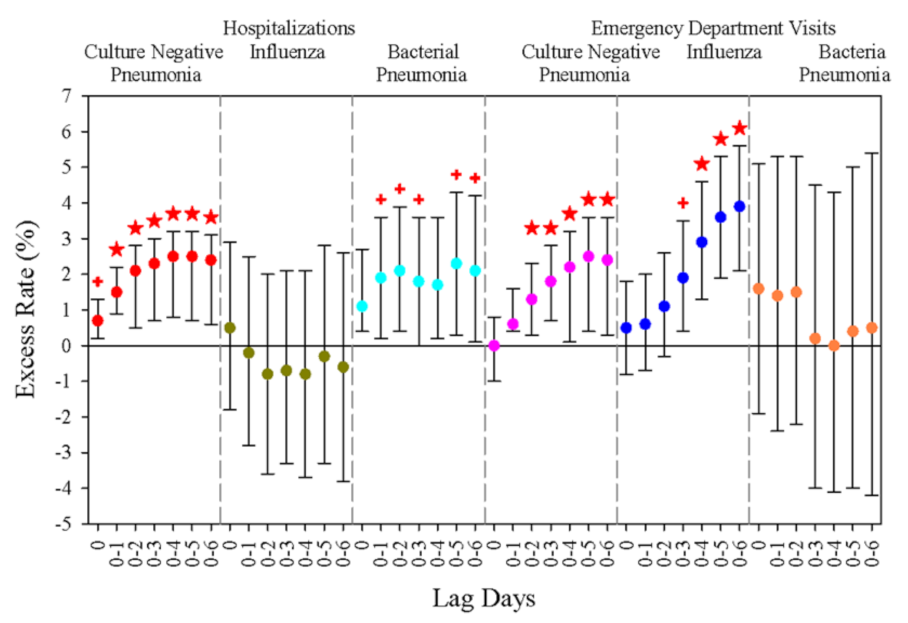
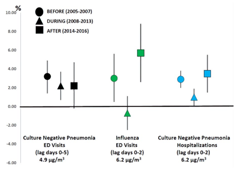
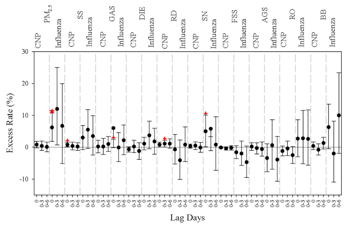
3.5.2. Respiratory Infections

Both emergency department (ED) visits and hospitalizations were investigated for respiratory infections [16]. The specific diseases were influenza, bacterial pneumonia, and culture negative pneumonia. Culture negative pneumonia is pneumonia in which culturing material from the patient cannot determine if the infection is caused by bacteria or virus. The excess rates of infectious disease hospitalizations associated with each IQR increase in PM2.5 are depicted in Figure 8. Hospitalizations for culture negative pneumonia were significantly associated with an IQR increase in PM2.5 for all lag days. Hospitalizations for bacterial pneumonia had statistically significant associations with IQR increases in PM2.5 for lag days 0–1 to 0–3 and for 0–5 and 0–6. For ED visits, culture negative pneumonia was strongly associated for lag days 0–2 to 0–6 and influenza was associated for lag days 0–3 to 0–6. The increase in ER with lag day is likely the result of the subject needing several days from the onset of these respiratory diseases before they recognized the need to seek medical assistance. Relative few influenza patients are hospitalized since it is typically sufficiently mild that they can be sent home to wait out the infection.
The differences in the ER values across the three periods were also examined and the values that showed a significant difference among the periods are shown in Figure 9. The ERs for culture negative pneumonia ED visits dropped from before to during, but they remained constant between during and after. However, influenza ED visits and culture negative pneumonia hospitalizations had a very different pattern with a sharp drop from before to during and a sharp rise from during to after. These two outcomes follow the pattern of the SOC distributions [9], suggesting a role for exposure to oxidants as a driver in the increased rates of infections.
To further explore these differences, source specific ER values were estimated [19] and the results are presented in Figure 10. Only culture negative pneumonia (CNP) and influenza ED visits have sufficient data to provide adequate power to observe possible associations. However, the relationships between the source-specific PM2.5 and ED visits for these respiratory infections are not as clearly defined. The strongest association was influenza with SS and the second highest was culture negative pneumonia with SN at lag 0. There were also significant values for GAS and influenza at lag 0 and RD with influenza at lag days 0–3. Short-term increases in PM2.5 from traffic and other combustion sources appear to be a potential risk factor for increased rates of influenza hospitalizations and ED visits.

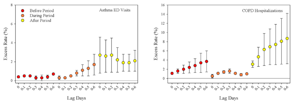
3.5.3. Respiratory Diseases

The respiratory diseases that had sufficient cases to be evaluated were asthma and chronic obstructive pulmonary disease (COPD) [17]. The excess rates of hospitalizations and ED visits for adult asthma and COPD declined during the period of 2005 to 2016 in parallel to the PM2.5 concentrations across NYS. However, the rate of COPD hospitalizations and ED visits for asthma per IQR increase in PM2.5 concentration increased in the after years (2014–2016) compared to the earlier periods (Figure 11). For example, each 6.8 μg/m3 increase in PM2.5 on the same day as the hospitalization or ED visit was associated with 0.4% (0.0%, 0.8%), 0.3% (−0.2%, 0.7%), and 2.7% (1.9%, 3.5) increases in the rate of asthma emergency department visits in the before, during, and after periods, respectively, suggesting the same PM2.5 mass concentration had increased toxicity in the after period.
The source-specific PM2.5 results for asthma hospitalizations [20] showed an increasing influence of secondary nitrate across the 3 periods with higher excess rates in the 0–3 and 0–6 lag-day results. There were also increased excess rates for secondary sulfate in the after period for these same lag days for both ED visits and hospitalizations. GAS, DIE, RO, BB, and FSS showed no significant excess rate values across periods or lag days. RD influenced both hospitalizations and ED visits across the periods with the highest values in the before period. AGS had increased excess rates in the after period with higher values for the 0–3 and 0–6 lag-day results. The source specific PM2.5 results for COPD [20] showed increased associations with excess rates of hospitalizations for spark- and compression ignition vehicles in the 2014–2016 period, but the values were not statistically significant. Other source types showed inconsistent patterns of excess rates. Overall, the relationships of asthma and COPD exacerbation with source-specific PM2.5 were not well defined and further work will be needed to determine the causes of the apparent increases in the per unit mass toxicity of PM2.5 for respiratory diseases in the 2014–2016 period.

4. Discussion

4.1. Changes in PM2.5 Composition

The reductions in sulfate and nitrate measured in the PM2.5 closely followed the reductions in emissions of SO2 and NOx, respectively [3,4,5]. The precursor gases react more quickly with hydroxyl radicals than with organic species, so the reductions in SO2 and NOx would allow more reactions with VOCs and IVOCs to produce additional SOAs as was observed between the during and after periods [9]. Primary organic carbon declined across the period, but SOAs declined from before to during and then rose in the after period. It is likely that some of the SOAs attributed to the before period may have been oxidized primary organic carbon (OPOC) as noted by Robinson et al. [43]. Li et al. [44] found significant water-soluble and humid-like organic carbon (HULIS) emitted from wood combustion in Chinese residential stoves particularly in the start-up and burn-out phases of the burn cycle. Thus, SOA-like materials can be directly emitted or formed through the reaction of oxidants with the primary organic aerosol constituents. These substances would include reactive oxygen species, such as peroxy and alkoxy radicals and peroxides [45].
Other source changes, such as the reduced use of No. 6 oil for heating in NYC, resulted in substantial decreases in the concentrations of Ni and V, typical tracers for residual oil combustion. At the same time as the phase out of No. 6 heating oil, the North American Emissions Control Area regulations [46] were forcing reductions in marine diesel fuel sulfur content. As of 2021, the fuel sulfur content had to be below 1% and as of 2015, it had to be below 0.1%, meaning that, in most cases, ships had to switch to burning No. 2 oil as the came into the Port of Elizabeth, NJ, USA.

4.2. Changes in Health Outcomes

Both ambient PM2.5 concentrations and hospitalization rates of cardiovascular events decreased across the study period (2005 to 2016), and the rate of hospitalizations for most cardiovascular disease subgroups associated with each interquartile range increase in PM2.5 concentration was not different after the environmental policies were implemented. There was a higher rate of ischemic heart disease and myocardial infarction associated with increased PM2.5 concentrations after these environmental policies were implemented and an economic recession occurred (2014 to 2016), in both the Upstate and New York City sites, compared to previous years (i.e., 2005–2007 and 2008–2013). The changes in PM composition and sources suggest that the shift from sulfate, nitrate, and primary organic carbon to more secondary organic carbon would represent an increase in oxidants associated with the PM [47,48] that can deliver ROS directly to the respiratory tract. The HULIS-like constituents would provide oxidative potential that can induce ROS in the lung fluid [49]. The strong oxidants associated with SOC in the particles have the ability to induce oxidative stress may be particularly important with regard to the triggering of acute cardiovascular events, such as myocardial infarctions [48].
The results for respiratory infections and diseases show some similar trends, but without as clear patterns as was observed in the CVD results. However, it appears that the potential increase in exposure to oxidative species is likely to be a major driver of the increased per unit mass toxicity in the after period. There are prior studies showing the effects of oxidative stress on the reduction in resistance to infection and the resulting increase in disease (e.g., [50,51]).
For respiratory diseases, there were clear increases in the toxicity per unit PM2.5 mass concentration for both asthma and COPD. However, the attribution of the increased effects to specific sources was less clear than for the other disease categories. A study in Los Angeles [52] reported temporal changes in the risk of CVD and asthma ED visits associated with short-term increases in ambient PM2.5 concentrations in the period of 2005 to 2016, and changes in PM2.5 composition (e. g., an increasing fraction of organic carbon and a decreasing fraction of sulfate in PM2.5). In general, there were fewer cases of respiratory diseases relative to the numbers of CVD or infections that resulted in ED visits or hospitalizations. The effects of these changes in toxicity per unit mass on the numbers of hospitalizations and emergency department visits have been reported by Hopke and Hill [53]. They concluded that, for some of the outcomes, the increased toxicity per unit mass reduced the benefits of the overall decline in PM2.5 concentrations. Indirectly, this implies that the PM2.5 chemistry is changing with changing emissions (urban air reactants) and needs further investigation.
There have been few similar studies that have examined changes in PM2.5 source contributions and resulting changes in adverse health outcomes. In Atlanta, the health benefits of pollution control policies were estimated for the period of 1999–2013 [54,55,56]. They found significant decreases in both PM2.5 and cardiorespiratory ED visits with no indication that the changing PM composition resulted in a change in per unit mass toxicity. However, Bi et al. [55] reported a study in Los Angeles during the period of 2005 to 2016 in which there were increases in the per unit mass toxicity with respect to CVD ED visits. They also related the change to the increasing fraction of OC in the residual PM2.5 after the reductions in sulfate and nitrate. The Bi et al. study as well as the NYS studies included the period after 2013 and the termination of the Atlanta study, suggesting that source and atmospheric chemistry changes in the most recent years (2014 to 2016) were related to the changes in PM toxicity.

5. Conclusions

The effects of the various federal regulations along with the fuel shift in electricity generation operations to natural gas driven by economic considerations were implemented to substantially reduce PM2.5 concentrations across New York State with concomitant reductions in ED visits and hospitalizations for cardiovascular and respiratory diseases and respiratory infections. However, there appear to be some unintended consequences of the shift in light-duty engine technology from PFI to GDI engines when coupled with the reformulation of gasoline to reduce its benzene content. This combination may have increased the potential emission of IVOCs, which with the increased availability of oxidants that were not used to oxidize NOx and SO2 led to increases in SOAs and related atmospheric ROS. The higher content of exogenous and endogenous ROS associated with the PM2.5 in the most recent period could be the cause of the increased per unit mass toxicity of the remaining PM2.5. Prior work [41,42] has suggested that the introduction of Tier 3 light-duty vehicles should result in lowered emissions of IVOCs and resulting concentrations of SOAs. Thus, the regulatory processes already in place may be sufficient to reduce the observed increased toxicity, but only additional health effect studies in the future will be able to determine if this improvement has been realized. The results for post 2005 changes in PM2.5 chemistry driven by changes in emissions from regulatory and economic directions is a good example of the changing urban air chemistry seen in the U.S. One can expect that further changes from emission management can be expected with shifts to renewable electricity generation and evolving low or zero emissions transportation technology.

Author Contributions

This review article was jointly written by P.K.H. and G.H. All authors have read and agreed to the published version of the manuscript.

Funding

The research summarized in this work was supported by the New York State Energy Research and Development Authority under contracts #59800, 59802, and 100412.

Institutional Review Board Statement

Not applicable.

Informed Consent Statement

Not applicable.

Acknowledgments

The work in New York State that was reviewed in this paper was supported by the New York State Energy Research and Development Authority under contract numbers 59800, 59802, and 100412.

Conflicts of Interest

The authors declare no conflict of interest.

References

  1. U.S. Environmental Protection Agency (US EPA). Inhalable Particulate Network Annual Report: Operation and Data Summary (Mass Concentrations Only); April 1979–June 1980, Report No. EPA-600/4-81-037; US Environmental Protection Agency: Washington, DC, USA, 1981; p. 265.
  2. Particulate Matter (PM2.5) Trends. Available online: https://www.epa.gov/air-trends/particulate-matter-pm25-trends (accessed on 21 December 2021).
  3. Squizzato, S.; Masiol, M.; Rich, D.Q.; Hopke, P.K. PM2.5 and gaseous pollutants in New York State during 2005–2016: Spatial variability, temporal trends, and economic influences. Atmos. Environ. 2018, 183, 209–224. [Google Scholar] [CrossRef]
  4. Blanchard, C.L.; Shaw, S.L.; Edgerton, E.S.; Schwab, J.J. Emission influences on air pollutant concentrations in New York State: I. ozone. Atmos. Environ. X 2019, 3, 100033. [Google Scholar] [CrossRef]
  5. Blanchard, C.L.; Shaw, S.L.; Edgerton, E.S.; Schwab, J.J. Emission influences on air pollutant concentrations in New York state: II. PM2.5 organic and elemental carbon constituents. Atmos. Environ. X 2019, 3, 100039. [Google Scholar] [CrossRef]
  6. Pitiranggon, M.; Johnson, S.; Haney, J.; Eisl, H.; Ito, K. Long-term trends in local and transported PM2.5 pollution in New York City. Atmos. Environ. 2021, 248, 118238. [Google Scholar] [CrossRef]
  7. Squizzato, S.; Masiol, M.; Rich, D.Q.; Hopke, P.K. A long-term source apportionment of PM2.5 in New York State during 2005–2016. Atmos. Environ. 2018, 192, 35–47. [Google Scholar] [CrossRef]
  8. Masiol, M.; Squizzato, S.; Rich, D.Q.; Hopke, P.K. Long-term trends (2005–2016) of source apportioned PM2.5 across New York State. Atmos. Environ. 2019, 201, 110–120. [Google Scholar] [CrossRef]
  9. Zhang, W.; Lin, S.; Hopke, P.K.; Thurston, S.W.; Van Wijngaarden, E.; Croft, D.; Squizzato, S.; Masiol, M.; Rich, D.Q. Triggering of cardiovascular hospital admissions by fine particle concentrations in New York state: Before, during, and after implementation of multiple environmental policies and a recession. Environ. Pollut. 2018, 242, 1404–1416. [Google Scholar] [CrossRef]
  10. Rich, D.Q.; Zhang, W.; Shao, L.; Squizzato, S.; Thurston, S.W.; van Wijngaarden, E.; Croft, D.; Masiol, M.; Hopke, P.K. Triggering of cardiovascular hospital admissions by source specific fine particle concentrations in urban centers of New York State. Environ. Int. 2019, 126, 387–394. [Google Scholar] [CrossRef]
  11. Solomon, P.A.; Crumpler, D.; Flanagan, J.B.; Jayanty, R.K.M.; Rickman, E.E.; McDade, C.E.U.S. National PM2.5Chemical Speciation Monitoring Networks—CSN and IMPROVE: Description of networks. J. Air Waste Manag. Assoc. 2014, 64, 1410–1438. [Google Scholar] [CrossRef] [Green Version]
  12. R Core Team. R: A Language and Environment for Statistical Computing; R Foundation for Statistical Computing: Vienna, Austria, 2017; Available online: https://www.R-project.org/ (accessed on 21 December 2021).
  13. Carslaw, D.C.; Ropkins, K. Openair—An R package for air quality data analysis. Environ. Model. Softw. 2012, 27–28, 52–61. [Google Scholar] [CrossRef]
  14. Maclure, M. 1991. The case-crossover design: A method for studying transient effects on the risk of acute events. Am. J. Epidemiol. 1991, 133, 144e153. [Google Scholar] [CrossRef] [PubMed]
  15. Levy, D.; Lumley, T.; Sheppard, L.; Kaufman, J.; Checkoway, H. Referent Selection in Case-Crossover Analyses of Acute Health Effects of Air Pollution. Epidemiology 2001, 12, 186–192. [Google Scholar] [CrossRef] [PubMed]
  16. Croft, D.P.; Zhang, W.; Lin, S.; Thurston, S.W.; Hopke, P.K.; Masiol, M.; Squizzato, S.; Van Wijngaarden, E.; Utell, M.J.; Rich, D.Q. The Association between Respiratory Infection and Air Pollution in the Setting of Air Quality Policy and Economic Change. Ann. Am. Thorac. Soc. 2019, 16, 321–330. [Google Scholar] [CrossRef] [PubMed]
  17. Hopke, P.K.; Croft, D.; Zhang, W.; Shao, L.; Masiol, M.; Squizzato, S.; Thurston, S.W.; van Wijngaarden, E.; Utell, M.J.; Rich, D.Q. Changes in the acute response of respiratory disease to PM2.5 in New York state from 2005 to 2016. Sci. Total Environ. 2019, 677, 328–339. [Google Scholar] [CrossRef] [PubMed]
  18. Croft, D.P.; Zhang, W.; Lin, S.; Thurston, S.W.; Hopke, P.K.; Van Wijngaarden, E.; Squizzato, S.; Masiol, M.; Utell, M.J.; Rich, D.Q. The associations between source specific particulate matter and of respiratory infections in New York state adults. Environ. Sci. Technol. 2020, 54, 975–984. [Google Scholar] [CrossRef] [PubMed] [Green Version]
  19. Hopke, P.K.; Croft, D.; Zhang, W.; Shao, L.; Masiol, M.; Squizzato, S.; Thurston, S.W.; van Wijngaarden, E.; Utell, M.J.; Rich, D.Q. Changes in the hospitalization and ED visit rates for respiratory diseases associated with source-specific PM2.5 in New York State from 2005 to 2016. Environ. Res. 2020, 181, 108912. [Google Scholar] [CrossRef]
  20. U.S. EPA. Finding of Significant Contribution and Rulemaking for Certain States in the Ozone Transport Assessment Group Region for Purposes of Reducing Regional Transport of Ozone. Fed. Regist. 1998, 63, 57356–57538. [Google Scholar]
  21. Napolitano, S.; Stevens, G.; Schreifels, J.; Culligan, K. The NOx Budget Trading Program: A Collaborative, Innovative Approach to Solving a Regional Air Pollution Problem. Electr. J. 2007, 20, 65–76. [Google Scholar] [CrossRef]
  22. U.S. EPA. Cross-state Air Pollution Rule Update for the 2008 Ozone NAAQS. Fed. Regist. 2015, 80, 75706–75778. [Google Scholar]
  23. U.S. EPA. Cross-state Air Pollution Rule Update for the 2008 Ozone NAAQS. Fed. Regist. 2016, 81, 74504–74650. [Google Scholar]
  24. U.S. EPA. Revised Cross-State Air Pollution Rule Update for the 2008 Ozone NAAQS. Fed. Regist. 2021, 86, 23054–23235. [Google Scholar]
  25. U.S. Department of Justice. 2007. Available online: https://www.justice.gov/enrd/us-v-american-elect-power-co (accessed on 21 December 2021).
  26. U.S. EPA. Control of Air Pollution from New Motor Vehicles: Tier 2 Motor Vehicle Emissions Standards and Gasoline Sulfur Control Requirements. Fed. Regist. 2000, 65, 6698–6870. [Google Scholar]
  27. U.S. EPA. Control of Emissions of Air Pollution From 2004 and Later Model Year Heavy-Duty Highway Engines and Vehicles; Revision of Light-Duty Truck Definition. Fed. Regist. 1999, 64, 58472–58566. [Google Scholar]
  28. U.S. EPA. Highway and Nonroad, Locomotive, and Marine (NRLM) Diesel Fuel Sulfur Standards. Office of Transportation and Air Quality EPA-420-B-16–1005. 2016. Available online: https://nepis.epa.gov/Exe/ZyPDF.cgi?Dockey=P100O9ZI.pdf (accessed on 21 December 2021).
  29. U.S. EPA. Control of Emissions of Air Pollution from Nonroad Diesel Engines and Fuel; Final Rule. Fed. Regist. 2004, 69, 38958–39273. [Google Scholar]
  30. Kheirbek, I.; Haney, J.; Douglas, S.; Ito, K.; Caputo, S., Jr.; Matte, T. The public health benefits of reducing fine particulate matter through conversion to cleaner heating fuels in New York City. Environ. Sci. Technol. 2014, 48, 13573–13582. [Google Scholar] [CrossRef] [PubMed]
  31. Theil, H. A Rank-Invariant Method of Linear and Polynomial Regression Analysis. In Henri Theil’s Contributions to Economics and Econometrics; Springer: Dordrecht, The Netherlands, 1992; pp. 345–381. [Google Scholar]
  32. Sen, P.K. Estimates of the regression coefficient based on Kendall’s tau. J. Am. Stat. Assoc. 1968, 63, 1379–1389. [Google Scholar] [CrossRef]
  33. Chow, J.C.; Watson, J.G.; Chen, L.-W.A.; Chang, M.C.O.; Robinson, N.F.; Trimble, D.; Kohl, S. The IMPROVE_A Temperature Protocol for Thermal/Optical Carbon Analysis: Maintaining Consistency with a Long-Term Database. J. Air Waste Manag. Assoc. 2007, 57, 1014–1023. [Google Scholar] [CrossRef] [Green Version]
  34. Kim, E.; Hopke, P.K.; Edgerton, E.S. Improving Source Identification of Atlanta Aerosol Using Temperature-Resolved Carbon Fractions in Positive Matrix Factorization. Atmos. Environ. 2004, 38, 3349–3362. [Google Scholar] [CrossRef]
  35. Kim, E.; Hopke, P.K. Source apportionment of fine particles at Washington, DC utilizing temperature resolved carbon fractions. J. Air Waste Manage. Assoc. 2004, 54, 773–785. [Google Scholar] [CrossRef] [PubMed]
  36. Wang, Y.; Hopke, P.K.; Rattigan, O.V.; Chalupa, D.C.; Utell, M.J. Multiple-year black carbon measurements and source apportionment using delta-C in Rochester, New York. J. Air Waste Manag. Assoc. 2012, 62, 880–887. [Google Scholar] [CrossRef] [PubMed] [Green Version]
  37. Wang, Y.; Hopke, P.K.; Xia, X.; Rattigan, O.V.; Chalupa, D.C.; Utell, M.J. Source apportionment of airborne particulate matter using inorganic and organic species as tracers. Atmos. Environ. 2012, 55, 525–532. [Google Scholar] [CrossRef]
  38. Kim, E.; Hopke, P.K. Improving source identification of fine particles in a rural northeastern U.S. area utilizing temperature resolved carbon fractions. J. Geophys. Res. 2004, 109, D09204. [Google Scholar] [CrossRef]
  39. Kruskal, W.H.; Wallis, W.A. Use of Ranks in One-Criterion Variance Analysis. J. Am. Stat. Assoc. 1952, 47, 583–621. [Google Scholar] [CrossRef]
  40. Zhao, Y.; Lambe, A.T.; Saleh, R.; Saliba, G. Secondary Organic Aerosol Production from Gasoline Vehicle Exhaust: Effects of Engine Technology, Cold Start, and Emission Certification Standard. Environ. Sci. Technol. 2018, 52, 1253–1261. [Google Scholar] [CrossRef]
  41. Zhao, Y.L.; Hennigan, C.J.; May, A.A.; Tkacik, D.S.; de Gouw, J.A.; Gilman, J.B.; Kuster, W.C.; Borbon, A.; Robinson, A.L. Intermediate-Volatility Organic Compounds: A Large Source of Secondary Organic Aerosol. Environ. Sci. Technol. 2014, 48, 13743–13750. [Google Scholar] [CrossRef]
  42. Lim, H.-J.; Turpin, B.J. Origins of Primary and Secondary Organic Aerosol in Atlanta: Results of Time-Resolved Measurements during the Atlanta Supersite Experiment. Environ. Sci. Technol. 2002, 36, 4489–4496. [Google Scholar] [CrossRef]
  43. Robinson, A.L.; Donahue, N.M.; Shrivastava, M.; Weitkamp, E.A.; Sage, A.M.; Grieshop, A.P.; Lane, T.E.; Pierce, J.R.; Pandis, S.N. Rethinking Organic Aerosol: Semivolatile Emissions and Photochemical Aging. Science 2007, 315, 1259–1262. [Google Scholar] [CrossRef]
  44. Li, X.; Han, J.; Hopke, P.K.; Hu, J.; Shu, Q.; Chang, Q.; Ying, Q. Quantifying primary and secondary humic-like substances in urban aerosol based on emission source characterization and a source-oriented air quality model. Atmos. Chem. Phys. 2019, 19, 2327–2341. [Google Scholar] [CrossRef] [Green Version]
  45. Hopke, P.K. Chapter 1: Reactive ambient particles. In Air Pollution and Health Effects, Molecular and Integrative Toxicology; Nadadur, S.S., Hollingsworth, J.W., Eds.; Springer: London, UK, 2015; pp. 1–24. [Google Scholar]
  46. Anastasopolos, A.T.; Sofowote, U.M.; Hopke, P.K.; Rouleau, M.; Shin, T.; Dheri, A.; Peng, H.; Kulka, R.; Gibson, M.D.; Farah, P.-M.; et al. Air quality in Canadian port cities after regulation of low-sulphur marine fuel in the North American Emissions Control Area. Sci. Total. Environ. 2021, 791, 147949. [Google Scholar] [CrossRef]
  47. Docherty, K.S.; Wu, W.; Lim, Y.B.; Ziemann, P.J. Contributions of organic peroxides to secondary organic aerosol formed from reactions of monoterpenes with O3. Environ. Sci. Technol. 2005, 39, 4049–4059. [Google Scholar] [CrossRef]
  48. Chen, X.; Hopke, P.K.; Carter, W.P.L. Secondary organic aerosol from ozonolysis of biogenic volatile organic compounds: Chamber studies of particle and reactive oxygen species formation. Environ. Sci. Technol. 2010, 45, 276–282. [Google Scholar] [CrossRef] [PubMed]
  49. Ma, Y.; Cheng, Y.; Qiu, X.; Cao, G.; Fang, Y.; Wang, J.; Zhu, T.; Yu, J.; Hu, D. Sources and oxidative potential of water-soluble humic-like substances (HULISWS) in fine particulate matter (PM2.5) in Beijing. Atmos. Chem. Phys. 2018, 18, 5607–5617. [Google Scholar] [CrossRef] [Green Version]
  50. Sarkar, K.; Sil, P.C. Infectious Lung Diseases and Endogenous Oxidative Stress. Oxidative Stress Lung Dis. 2019, 2, 125–148. [Google Scholar]
  51. Kozlov, E.M.; Ivanova, E.; Grechko, A.V.; Wu, W.-K.; Starodubova, A.V.; Orekhov, A.N. Involvement of Oxidative Stress and the Innate Immune System in SARS-CoV-2 Infection. Diseases 2021, 9, 17. [Google Scholar] [CrossRef] [PubMed]
  52. Bi, J.; D’Souza, R.R.; Rich, D.Q.; Hopke, P.K.; Russell, A.G.; Liu, Y.; Chang, H.H.; Ebelt, S. Temporal changes in short-term associations between cardiorespiratory emergency department visits and PM2.5 in Los Angeles, 2005 to 2016. Environ. Res. 2020, 190, 109967. [Google Scholar] [CrossRef] [PubMed]
  53. Hopke, P.K.; Hill, E.L. Health and charge benefits from decreasing PM2.5 concentrations in New York State: Effects of changing compositions. Atmos. Pollut. Res. 2021, 12, 47–53. [Google Scholar] [CrossRef]
  54. Abrams, J.Y.; Klein, M.; Henneman, L.R.F.; Sarnat, S.E.; Chang, H.H.; Strickland, M.J.; Mulholland, J.A.; Russell, A.G.; Tolbert, P.E. Impact of air pollution control policies on cardiorespiratory emergency department visits, Atlanta, GA, 1999–2013. Environ. Int. 2019, 126, 627–634. [Google Scholar] [CrossRef] [PubMed]
  55. Henneman, L.R.F.; Liu, C.; Chang, H.; Mulholland, J.; Tolbert, P.; Russell, A. Air quality accountability: Developing long-term daily time series of pollutant changes and uncertainties in Atlanta, Georgia resulting from the 1990 Clean Air Act Amendments. Environ. Int. 2019, 123, 522–534. [Google Scholar] [CrossRef]
  56. Russell, A.G.; Tolbert, P.E.; Henneman, L.R.F.; Abrams, J.; Liu, C.; Klein, M.; Mulholland, J.A.; Sarnat, S.; Hu, Y.; Chang, H.H.; et al. Impacts of regulations on air quality and emergency department visits in the Atlanta metropolitan area, 1999–2013. In Research Report 195; Health Effects Institute: Boston, MA, USA, 2018. [Google Scholar]
Figure 1. Box and whisker plots describing the source contribution distributions for secondary sulfate. The bar in the box represents the median value and the circle represents the mean value.
Atmosphere 13 00193 g001
Figure 2. Box and whisker plots describing the source contribution distributions for secondary nitrate. The bar in the box represents the median value and the circle represents the mean value.
Atmosphere 13 00193 g002
Figure 3. Box and whisker plots describing the source contribution distributions for gasoline vehicle emissions. The bar in the box represents the median value and the circle represents the mean value.
Atmosphere 13 00193 g003
Figure 4. Box and whisker plots describing the source contribution distributions for diesel vehicle emissions. The bar in the box represents the median value and the circle represents the mean value.
Atmosphere 13 00193 g004
Figure 5. Excess rates (%) for cardiovascular hospitalizations per interquartile range of PM2.5 over the whole study period.
Atmosphere 13 00193 g005
Figure 6. Plot of excess rates (%) for an increase in the IQR for each of the cardiovascular outcomes in the Before (top), During (middle) and After (bottom) periods.
Atmosphere 13 00193 g006
Figure 7. Excess rates for various cardiovascular diseases associated with the IQR increases in source-specific PM2.5 concentrations. * indicates statistical significance at p < 0.016.
Atmosphere 13 00193 g007
Figure 8. Excess rates (%) of respiratory infections per IQR increase in PM2.5 for the various lag days. The indicates a p-value < 0.001. The indicates p-values between 0.01 and 0.05.
Atmosphere 13 00193 g008
Figure 9. Excess rate (%) for those respiratory infections with significant changes among the 3 periods.
Atmosphere 13 00193 g009
Figure 10. Excess rate (%) per IQR of source specific PM2.5 at various log days. The indicates a p-value < 0.001. The indicates p-values between 0.01 and 0.05.
Atmosphere 13 00193 g010
Figure 11. Excess rates (%) per IQR in PM2.5 concentrations across the three periods and lag days.
Atmosphere 13 00193 g011
Table 1. The linear trends statistics for PM2.5 calculated over the period and by season. Trends are expressed in percentage (%) y−1 along with the upper (u.ci) and lower (l.ci) 95th confidence intervals in the trends and the p-values, indicating the statistical significance of the slope estimates. Trends are statistically significant at p-value < 0.05 based on the Kendall–Mann test. Details are provided in Squizzato et al. [3].
SiteAllWinterSummerTransition
Slope (l.ci, u.ci; p-Value)
% y−1[Start Date–End Date]
Slope (l.ci, u.ci; p-Value)
% y−1[Start Date–End Date]
Slope (l.ci, u.ci; p-Value)
% y−1[Start Date–End Date]
Slope (l.ci, u.ci; p-Value)
% y−1[Start Date–End Date]
Albany−3.8 (−4.4, −3.1; 0)
[1 January 2005–12 January 2016]
−4.2 (−5.6, −2.5; 0)
[1 January 2005–12 January 2016]
−4.6 (−5.5, −3.4; 0)
[6 January 2005–8 January 2016]
−3.3 (−4.3, −2.5; 0)
[3 January 2005–11 January 2016]
Buffalo−3.7 (−4.1, −3.1; 0)
[1 January 2005–12 January 2016]
−4.2 (−5.2, −2.7; 0)
[1 January 2005–12 January 2016]
−4.3 (−5.6, −3.2; 0)
[6 January 2005–8 January 2016]
−3.7 (−4.6, −2.6; 0)
[3 January 2005–11 January 2016]
Rochester−3.4 (−3.9, −2.7; 0)
[1 January 2005–12 January 2016]
−3.3 (−4.7, −1.8; 0)
[1 January 2005–12 January 2016]
−4 (−5.4, −1.8; 0)
[6 January 2005–8 January 2016]
−3.6 (−4.6, −2.3; 0)
[3 January 2005–11 January 2016]
Manhattan−3.7 (−4.5, −2.8; 0)
[3 January 2007–12 January 2016]
−2.5 (−4.4, 0.4; 0.07)
[12 January 2007–12 January 2016]
−5.9 (−6.5, −3.3; 0)
[6 January 2007–8 January 2016]
−3.4 (−4.3, −2.4; 0)
[3 January 2007–11 January 2016]
Bronx−3.3 (−3.7, −2.5; 0)
[1 January 2005–12 January 2016]
−3.1 (−3.7, −2.3; 0)
[1 January 2005–12 January 2016]
−5 (−5.6, −4; 0)
[6 January 2005–8 January 2016]
−3.5 (−4.3, −2.7; 0)
[3 January 2005–11 January 2016]
Queens−3.9 (−4.3, −3.3; 0)
[1 January 2005–12 January 2016]
−3 (−4.3, −1.6; 0)
[1 January 2005–12 January 2016]
−4.8 (−5.4, −4.2; 0)
[6 January 2005–8 January 2016]
−3.6 (−4.4, −2.8; 0)
[3 January 2005–11 January 2016]
Table 2. Average source contributions (in µg/m3 ± standard deviation) on PM2.5 mass for each identified sources at each site.
SourceSecondary SulfateSecondary NitrateSpark-IgnitionDieselRoad DustBiomass BurningOP-RichAged Sea SaltRoad SaltFresh Sea SaltResidual OilIndustrial
Albany
pre-OC/EC change4.0 ± 5.51.6 ± 1.81.5 ± 1.51.9 ± 1.70.4 ± 0.50.5 ± 0.5 0.1 ± 0.3
post-OC/EC change2.1 ± 2.00.9 ± 1.32.2 ± 2.00.5 ± 0.30.2 ± 0.20.4 ± 0.51.2 ± 1.3 0.1 ± 0.5
Bronx
pre-OC/EC change4.3 ± 4.93.1 ± 3.91.5 ± 1.61.4 ± 1.00.3 ± 0.30.3 ± 0.5 0.8 ± 0.9 0.4 ± 1.11.0 ± 1.0
post-OC/EC change2.7 ± 3.50.7 ± 1.02.0 ± 1.90.8 ± 0.50.4 ± 0.40.1 ± 0.21.4 ± 1.80.4 ± 0.6 0.1 ± 0.31.0 ± 1.1
Buffalo
pre-OC/EC change4.4 ± 5.31.7 ± 2.21.2 ± 1.41.9 ± 1.60.2 ± 0.21.1 ± 1.1 0.5 ± 1.5 0.3 ± 0.3
post-OC/EC change2.6 ± 3.31.6 ± 2.41.5 ± 1.70.6 ± 0.40.2 ± 0.20.6 ± 0.70.9 ± 1.0 0.0 ± 0.1 0.2 ± 0.1
Manhattan
pre-OC/EC change4.5 ± 5.73.9 ± 4.41.0 ± 0.91.6 ± 1.21.0 ± 0.80.5 ± 0.7 0.7 ± 0.8 0.4 ± 1.00.6 ± 0.7
post-OC/EC change2.4 ± 2.71.1 ± 1.51.9 ± 2.01.3 ± 0.70.5 ± 0.50.3 ± 0.31.7 ± 2.30.6 ± 0.7 0.1 ± 0.20.6 ± 0.8
Queens
pre-OC/EC change4.7 ± 5.12.2 ± 2.71.5 ± 1.51.4 ± 1.10.5 ± 0.50.6 ± 0.7 0.3 ± 0.4 0.3 ± 0.70.4 ± 0.5
post-OC/EC change2.2 ± 2.31.1 ± 1.71.7 ± 1.60.7 ± 0.50.3 ± 0.30.3 ± 0.30.9 ± 1.00.6 ± 0.7 0.1 ± 0.20.4 ± 0.5
Rochester
pre-OC/EC change3.6 ± 4.62.6 ± 3.31.5 ± 1.40.4 ± 0.30.2 ± 0.20.8 ± 1.1 0.2 ± 0.3
post-OC/EC change2.1 ± 2.51.5 ± 2.31.4 ± 1.60.8 ± 0.60.1 ± 0.10.6 ± 0.50.6 ± 0.6 0.1 ± 0.2
Table 3. GDI Market Share, 2007–2016.
GDI Market Share
Model YearCarsLight Trucks
20070.3%0.00%
20083.1%1.10%
20094.2%4.20%
20109.2%6.8%
201118.4%11.3%
201227.4%13.5%
201337.3%18.4%
201442.7%29.7%
201544.0%39.0%
201650.7%43.2%
Publisher’s Note: MDPI stays neutral with regard to jurisdictional claims in published maps and institutional affiliations.

