High-Resolution Measurements of SO₂, HNO₃ and HCl at the Urban Environment of Athens, Greece: Levels, Variability and Gas to Particle Partitioning

Abstract

High-resolution measurements of sulfur dioxide (SO₂), nitric acid (HNO₃), and hydrochloric acid (HCl) were conducted in Athens, Greece, from 2014 to 2016 via a wet rotating annular denuder system paired with an ion chromatograph. Decreased mean annual levels of SO₂ and HNO₃ (equal to 3.3 ± 4.8 μg m⁻³ and 0.7 ± 0.6 μg m⁻³, respectively) were observed relative to the past, whereas for HCl (mean of 0.4 μg m⁻³ ) no such comparison was possible as the past measurements are very scarce. Regional and local emission sources regulated the SO₂ levels and contributed to both the December and the July maxima of 6.6 μg m⁻³ and 5.5 μg m⁻³, respectively. Similarly, the significant enhancement at noon and during the winter nighttime was due to transported SO₂ and residential heating, respectively. The oxidation of NO₂ by OH radicals and the heterogeneous reactions of HNO₃ on sea salt seemed to drive the HNO₃ and HCl formation, respectively, whereas nighttime biomass burning affected only the former by almost 50%. During summer, the sulfate anions dominated over the SO₂, in contrast to the chloride and nitrate ions that prevailed during the winter and were linked to the aerosol acidity that influences their lifetime as well as their impact on ecosystems.

1. Introduction

Nitric acid, hydrochloric acid, and sulfur dioxide (HNO₃, HCl, and SO₂, respectively) are the main atmospheric acidic gases that impact on the air quality and oxidative capacity of the atmosphere. HNO₃ is produced during the day mainly via the reaction of nitrogen dioxide (NO₂) with hydroxyl (OH) radicals [1]. Its nighttime formation includes the reaction of nitrate radicals (NO₃)—formed by the reaction of O₃ with NO₂ that no longer photolyzes—with volatile organic compounds (VOC) and the heterogeneous hydrolysis of nitrogen pentoxide (N₂O₅) [2]. The heterogeneous reactions of NO₃ radicals on particulates are considered of less importance compared to the other processes [3]. HNO₃ formation is also involved in ozone (O₃) production, thus serving as a sink for nitrogen oxides (NO_x). Annual levels of few pptv to several ppbv of HNO₃ might be encountered depending on the type of observation site, e.g., remote/clean versus urban/polluted conditions. HCl is emitted by the combustion of carbon- and chloride-containing fuels (e.g., solid waste combustion [4,5]), by water disinfection, and by manufacturing processes. It is also directly emitted by volcanoes, as well as by heterogeneous reactions on sea salt aerosol [6,7]. SO₂ is one of the major products of fossil fuel combustion, which is further oxidized, both via gas-phase and/or heterogeneous reactions, into sulfuric acid (H₂SO₄) and subsequently into sulfate (SO₄²⁻) particles, with the latter acting as cloud condensation nuclei (CCN), thus affecting the radiative forcing of the atmosphere. SO₂ can also be released by volcanoes or as a byproduct of the natural metabolism of dimethyl sulfide (DMS) in the marine environment [8].

Once released or formed in the atmosphere, these compounds are removed via wet or dry deposition or chemical reactions, either with gaseous ammonia (NH₃) and/or salts (e.g., CaCO₃, NaCl). Specifically, NH₃ is mainly emitted by fertilizers, animal waste, coal combustion, and the biomass burning of agricultural residuals, as well as from soil, vegetation, oceans, and traffic [9,10,11]. Ammonia selectively reacts with H₂SO₄ and, in the case of excess, reacts with HNO₃ and HCl, forming semi-volatile salts [12]. The acidity of the produced aerosol, which is also affected by other constituents, such as dust and potassium, along with temperature and relative humidity [13,14,15,16], regulates their partitioning into the gas or the particle phase. Therefore, there is a direct association between the levels of the gaseous aerosol precursors and the mass concentration and composition of the fine particles, which might be crucial for health protection [17] and the application of emission-control policies. In addition, the resulting acidification of precipitation, as well as the interaction of the acidic gases with the materials, has adverse effects on ecosystems and buildings, including culturally significant monuments.

Traditionally, denuder and/or filter-based techniques based on acquired samples are used to monitor inorganic aerosols and their gaseous precursors [18]. Longer sampling times, e.g., several hours, on filter packs may result in sampling artifacts, such as the evaporation of semi-volatile aerosol species such as nitrates or the absorption of inorganic gases such as nitric acid by the sampling media or particles. Efficient retention of trace gases can be achieved using denuders, where the gases are absorbed on a coating on the inner walls, and the particles are collected on the filters. Despite the effectiveness of capturing the time-weighed levels of the acidic compounds, the disadvantages of poor temporal resolution and the prolonged laboratory treatment make these methods difficult to deploy on a long-term basis, while the rapid changes of the chemical constituents cannot be identified. In recent years, various semi-continuous instruments have been developed to measure the chemical composition of atmospheric aerosols and/or their gaseous precursors, including the particle-into-liquid sampler (PILS-IC), the Ambient Ion Monitor-Ion Chromatograph system (AIM-IC), the Parallel Plate Wet Denuder and the Particle Into Liquid Sampler coupled with Ion Chromatography (PPWD-PILS-IC), and the Monitor for AeRosols and GAses in ambient air (MARGA), facilitating the monitoring of the inorganic atmospheric constituents with a higher time resolution [19,20,21,22,23,24,25,26,27,28].

At a European level, the EMEP network (European Monitoring and Evaluation Programme) registers the ambient levels of gaseous acidic compounds at several reference stations, providing long-term datasets, which have shown decreasing trends in the levels of oxidized sulfur and nitrogen compounds from 1990–2012 [29]. According to the recent report of the European Environment Agency [30] for the air quality in Europe, SO₂ concentrations were generally well below the limit values for the protection of human health during 2018, with the exception of some stations in the Balkans and Turkey. The trend analysis for the period of 2009–2018, included in the same report, shows that the highest average decreases in SO₂ concentrations were observed at industrial, urban, and suburban background stations, while the lowest decrease was observed at rural background stations maintaining in any case annual mean concentrations on 2018 of approximately 2–4 μg m⁻³, depending on the station type. The study by Tang et al. [31] on 64 sites of 20 cities from 2006–2010 reported higher SO₂ concentrations in central and eastern Europe. The highest levels were mainly encountered during the winter, with the exception of southern European sites that registered an enhancement in summer. Therefore, the expected winter enhancement due to domestic heating emissions might not be the case for all sites as the presence of other local emitters could contribute to its seasonal and diurnal variability, resulting in increased summer and daytime levels [32]. Despite the fact that SO₂ and NO₂ (the latter being considered as a precursor of HNO₃) are officially measured by national air quality monitoring networks, the measurements of HNO₃ and HCl are much less frequent. In addition, the majority of published works in southern Europe refer to measurements performed before 2000, utilizing low-resolution techniques or short-term measurement campaigns [33,34], which do not allow the investigation of the diurnal or long-term behavior of those acidic gases. Clear seasonal cycles with almost double the levels of HNO₃ in spring relative to winter (0.22 ± 0.19 ppb and 0.13 ± 0.12 ppb, respectively), a reverse trend for SO₂ (0.76 ± 1.00 ppb against 1.32 ± 1.73 ppb), and an insignificant variability for HCl (0.04 ± 0.11 ppb and 0.03 ± 0.08 ppb, respectively) were observed in Helsinki, Finland in 2009–2010, using a MARGA online monitor [35]. Five-year measurements in the rural field site of Melpitz, Germany from 2010–2014 produced daytime peaks for all three compounds, whereas the wintertime high concentrations of SO₂, due to elevated emissions from domestic heating and enrichment by the formation of an inversion layer, were in contrast with the HNO₃ and HCl maxima in the summer [36]. Tang et al. [31] reported HNO₃ maxima during the summer in eastern and southern Europe due to increased photochemistry, while there was no discernible seasonality for HCl.

The atmospheric composition, especially in Greek cities, has been altered during the last 20 years due to the improvement of urban air quality as a consequence of the adaptation of pollution-control measures and urban deindustrialization. However, the appearance of residential wood burning (RWB) since 2013, as a new source, has contributed to a long-term air quality deterioration in the winter months [37,38,39,40,41,42]. In terms of gaseous species, the impact of prevailing emission sources, such as traffic and RWB in Athens, has been assessed for non-methane hydrocarbons (NMHCs), highlighting the importance of the latter process [43]. In addition, α-pinene and limonene, which were expected to be of natural origin, also presented maxima during the cold period, which were attributable to anthropogenic production pathways, as in other works in urban areas [44,45,46]. As the changes in the type and strength of the emission sources are expected to also have a bearing on the levels of inorganic gaseous acidic compounds, relative to the past, the current work aims to: (i) provide information on the levels and variability of SO₂, HNO₃, and HCl under the current atmospheric conditions in the Greater Athens Area (GAA), using high-resolution measurement techniques that facilitate the investigation of their diurnal and seasonal patterns; (ii) assess the factors controlling their formation and removal, emphasizing the role of residential wood burning; and (iii) investigate the gas/particle partitioning of the various acidic compounds which can drive their fate and impacts on the atmosphere. The innovation of our work lies in the use for first time of a continuous denuder-based, high-resolution automated technique for the monitoring of HNO₃ and HCl in GAA, whereas the phase partitioning ratios from the concurrent measurements of both particulate and gaseous inorganic species are reported for first time, to our knowledge, for the Eastern Mediterranean. Finally, our measurements, apart from being valuable for atmospheric modelers, can fill a gap in the literature of more than 20 years on the levels of inorganic aerosol precursors in Greece.

2. Study Area and Measurements

2.1. Measurement Site

The measurements were conducted at the Thissio Air Monitoring station (37.9732° N, 23.7180° E) of the National Observatory of Athens, Greece. The sampling site, located at the top of the Hill of Nymphs, close to the historical center of the city, is ideal for the characterization of the urban background air pollution conditions [41,45], being thus representative of the typical population exposure to harmful pollutants in central Athens. As the station overlooks the city center, it serves as a receptor point, through the dispersion and circulation of pollutants from different potential sources. Monitoring of gaseous acidic compounds took place from December 2014 to February 2015, June to October 2015, and February to March 2016; these are periods typical of cold, warm, and transition seasons, respectively, considering that each one reflects contrasted air pollution profiles in terms of dominant emission sources and atmospheric processes, such as biomass burning, dust transport, or intense photochemistry.

2.2. Instrumentation

Real-time measurements of SO₂, HNO₃, and HCl were implemented by means of a Wet Annular Denuder system coupled with an Ion Chromatograph (WAD-IC). Diffusion-based sampling devices such as denuders and diffusion scrubbers are commonly used, as described in the introduction, as they allow the separation of gaseous and particulate matter during sampling. In our case, air was drawn at approximately 10 L min⁻¹ through the WAD concentric, rotating glass cylinders and mixed with ultrapure water to dissolve the gases. The sequential analysis of the samples was carried out by a Metrohm 761 compact Ion Chromatograph equipped with a Metrosep A Supp (4 mm) column and guard-column, on a 20 min basis. The separation of anions was conducted with isocratic elution of NaHCO₃ (3.4 mM)/Na₂CO₃ (3.6 mM) as an eluent and a flow of 0.4 mL min⁻¹. The reported concentrations were blank corrected. The calibration standards for the quantification were prepared twice for each period of measurements, in the range of 5 ppb to 350 ppb.

A Particle Into Liquid System combined with an Ion Chromatograph (PILS-IC) was used for highly time-resolved measurements of water-soluble inorganic chloride, nitrate, and sulfate anions (Cl⁻, NO₃⁻, and SO₄²⁻, respectively) [47,48] in the PM₁ fraction. For the determination of anions, a Dionex Ion Pac AS11 4mm (10–32) column and a Dionex Ion Pac AG11 4 mm (10–32) guard column were used with an ASRS-ULTRA II suppressor, under isocratic elution of NaHCO₃ (3.4 mM)/Na₂CO₃ (3.6 mM) as an eluent. The continuous flow of the aquatic solution was injected onto the chromatograph to determine the levels of anions on a 15 min resolution. The PILS sample ambient air flow rate was 16.7 L min⁻¹, and a cyclone was used to select PM₁ particles.

A portable aethalometer (AE-42; Magee Scientific) was operated for Black Carbon (BC) measurements at 7 wavelengths (370, 470, 520, 590, 660, 880, and 950 nm) on a 5 min resolution during the winter of 2014–2015. After corrections for multiple-scattering and shadowing effects, as described in [39,49,50,51], the 7-λ aethalometer measurements were decomposed to the BC fractions associated with fossil fuel combustion (BC_ff) and wood burning (BC_wb) [52]. Since May 2015, the BC levels of 1 min resolution have been derived from a AE-33 Magee Scientific dual-spot 7-λ aethalometer [53,54]. The BC_ff and BC_wb fractions were calculated based on the incorporated algorithm in the AE33, providing directly the biomass burning contribution (BB%) to BC. The 880 nm used as reference for the BC mass concentration, whereas the BC_wb and BC_ff components were calculated using the “Aethalometer model” [52] at 470-950 nm band, using Absorption Ångström Exponent (AAE) for wood burning and fossil fuel combustion equal to AAE_wb = 2 and AAE_ff = 1, respectively. Regulatory gaseous pollutants, namely nitrogen oxides (NO_x: NO, NO₂) and SO₂, were monitored at a 1 min resolution by Horiba 360 series automatic gas analyzers [55]. The meteorological data (temperature, relative humidity, solar radiation, precipitation, wind speed, and direction) were obtained by NOA’s automatic meteorological station at Thissio (1 min resolution) and averaged on 1 h intervals. Finally, the air mass origins for the measurement periods were identified by applying a 4-day back-trajectory analysis with the Hybrid Single-Particle Lagrangian Integrated Trajectory (HYSPLIT) model [56], in order to classify each day into dust and non-dust cases, considering also the levels of aluminum or calcium for the evaluation.

2.3. Box Modelling

Our chemical analysis has been complemented with a kinetic box model to determine the abundance of OH radicals. In short, the box model used includes hundreds of reactions, along with the critical heterogeneous ones, and the VOC oxidation schemes in the gas phase and the aqueous phase of the atmosphere are based on recent kinetic data. When experimental data are missing, the simulations are supplemented by contemporary simulations from the TM5MP chemistry transport model [57,58]. The TM5-MP is driven by meteorological fields from the ECMWF ERA-Interim reanalysis [59], and for this work, a spin-up time of 1 year was applied.

The simulations performed for this work are structured around the well-documented Carbon Bond Mechanism (CBM) that has been extensively used in chemistry modeling studies. The CBM considers all the major atmospheric reaction pathways of odd oxygen (Ox ≡ O + O₃) and NO_x, and the oxidation of VOCs, based on a lumped-structure approach. Specifically, we applied here the modified Carbon Bond Mechanism v5 (mCB05) [60]. A detailed description of the mCB05 is presented by Myriokefalitakis et al. [57].

The gas-phase chemical mechanism has been supplemented by an explicit multiphase scheme, both for cloud/fog water and aerosol water [58]. KPP version 2.2.3 [61,62] was used to generate the Fortran 90 code for the numerical integration of the gas- and the aqueous-phase chemical mechanisms. The Rosenbrock solver is used in this work as the numerical integrator [63]. Note, however, that for our kinetic modelling framework, only the integration method was used. To this end, all the gas- and aqueous-phase photolysis and thermal reactions and the mass transfer coefficients, along with the aerosol-dissolution processes, were provided to the aforementioned chemistry solver. More details are provided by Myriokefalitakis et al. [57,58]. Finally, we note that the box model’s photolysis frequencies are derived from the TM5MP model, calculated online using a band approach scheme [64].

3. Results and Discussion

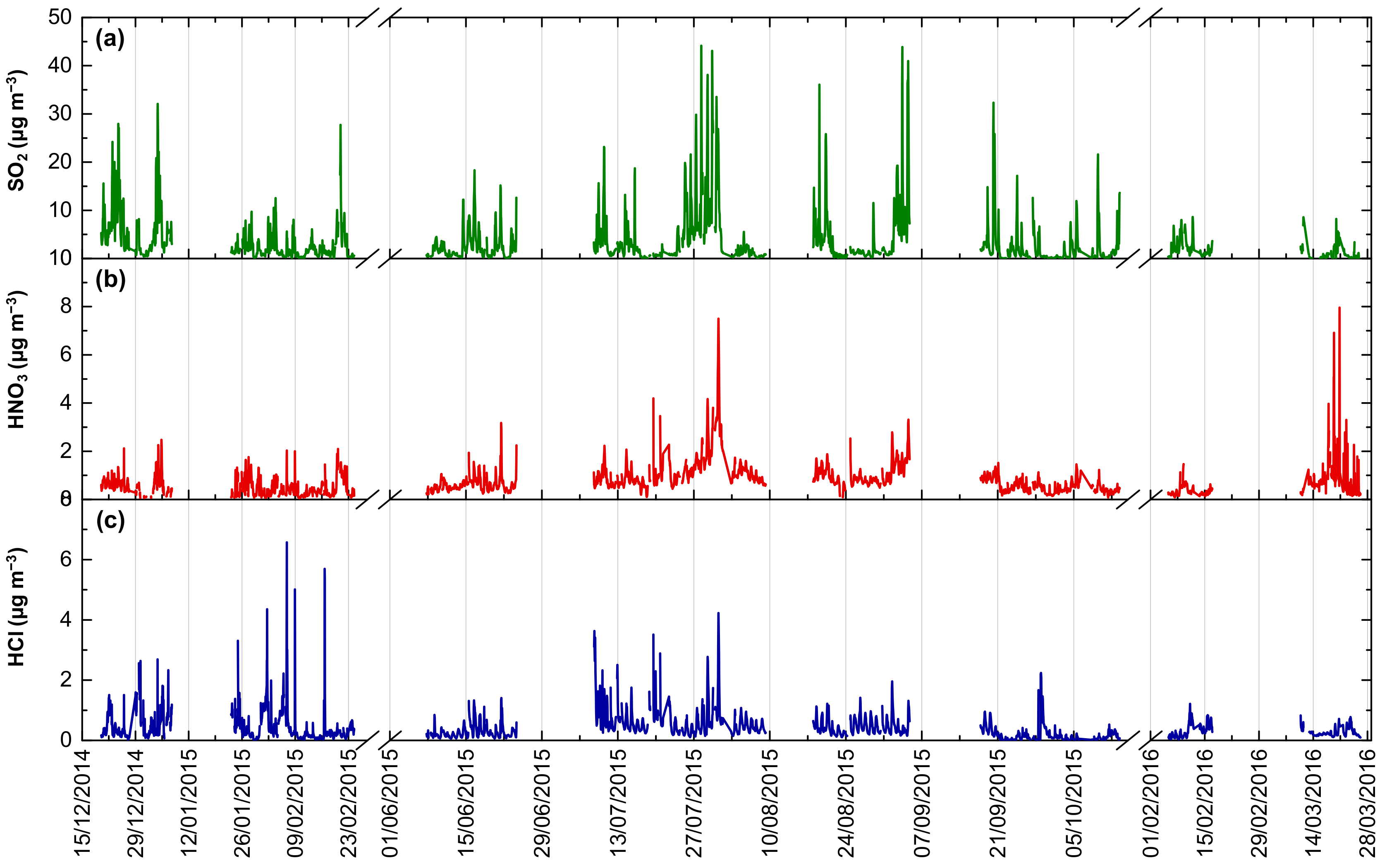
3.1. Temporal Variability of Acidic Gases

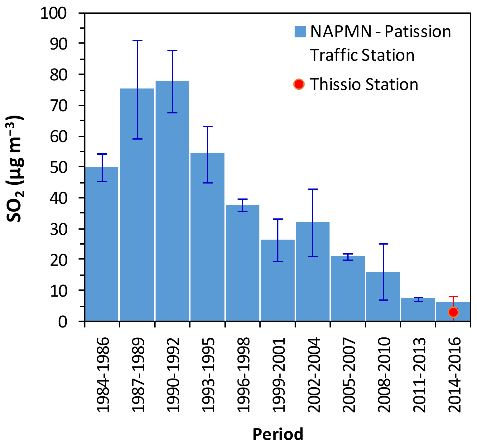
3.1.1. Levels and Comparison with Past Measurements

The mean hourly levels of the acidic gases measured during the selected periods are depicted in Figure 1, whereas

Table 1. Comparison of SO₂, HNO₃, and HCl levels (μg m⁻³) of the current study in Athens, Greece, over the period 2014–2016 with other environments in the Eastern and Central Mediterranean. Mean, standard deviation, and range are provided per case depending on the available records.

Site (Type: Period)	SO2	HNO3	HCl
Thissio, Athens, Greece 1 (Urban background: 2014–2016)	3.3 ± 4.8 (0.1–44.2)	0.7 ± 0.6 (0.1–8.0)	0.4 ± 0.5 (BDL 2–6.6)
Patission Station, Athens, Greece [76] (Urban Traffic: 2002–2004)		1.5 ± 1.2
Finokalia, Crete, Greece [65,73] (Remote coastal: 11/1996–9/1999	2.67 ± 0.88	1.20 ± 0.77
Patras, Greece [74] (Coastal: 11/1995–8/1996)		1.6–4.2
Erdemli, Turkey [66] (Coastal, rural: 1–2/2015 and 8–9/2015)	0.88 ± 1.33 (0.10–10.3)	0.35 ± 0.17 (0.055–1.44)
Ashdod, Israel [67] (Urban: 11–12/2004, 7/2005)	19.6 ± 19.8 18.0 ± 13.5	0.30 ± 0.19 0.61 ± 0.25	- 0.52 ± 0.17
Milan, Italy [68] (Central urban background: 6–7/2012)	2.41 ± 1.31	1.83 ± 1.31	0.28 ± 0.30

¹ Current work; ² BDL: Below Detection Limit.

presents the published values of the studies in the Eastern and Central Mediterranean. Regarding the SO₂ measurements, a collocated automatic UV fluorescence analyzer was also operated for short periods, for quality control purposes. The comparison of the two techniques exhibited strong agreement, with a regression slope close to unity and a squared correlation coefficient of r² = 0.88 (Figure S1a,b, respectively), indicating the reliable operation of the WAD-IC system.

The SO₂ measurements exhibited a mean value of 3.3 ± 4.8 μg m⁻³, with mean hourly peaks exceeding 15 μg m⁻³ throughout the year and maxima close to 44 μg m⁻³ in the summer and early fall (Figure 1). Compared with the long-term measurements conducted at a regional background location on the island of Crete in the late 1990s [65] or with other more recent records at coastal background sites such as Erdemli, Turkey [66], the levels in Athens were higher by 25% to 4 times, reflecting the different local emission sources and the different degrees of regional SO₂ influence. Nevertheless, by focusing on urban locations and comparing with Ashdod, Israel [67], or Milan [68], the SO₂ levels in Athens ranged in between.

Furthermore, according to a climatological analysis [69] for the central, most polluted urban stations in Athens over the period of 1987–1997, a decrease of 52% in the SO₂ levels at the Patission traffic station (located at one of the most congested streets of Attica) was reported between 1988–1990 and 1995–1997 (83 ± 4 μg m⁻³ and 40 ± 4 μg m⁻³, respectively) and is attributed to the application of abatement measures over the period of 1991–1994. The mean annual roadside levels of SO₂ further decreased to about 14 μg m⁻³ in 2009 [70] and 8 μg m⁻³ in 2019 [71]. These additional reductions in SO₂ levels can be attributed to the deindustrialization in the GAA and, on a national level, to the application of abatement measures and the reduction in emissions due to the recession after 2008 [72]. The mean level at about 3 μg m⁻³, observed at Thissio in 2014–2016, taking into account its standard deviation, falls within the range of the mean levels of 4–8 μg m⁻³ reported for the Patission station for the respective time period (Figure 2). Considering that the Patission station is located at one of the most congested streets of the GAA, the above agreement indicates the mostly regional character of SO₂.

The hourly concentrations of HNO₃ varied from 0.1 μg m⁻³ to almost 8 μg m⁻³, with a mean of 0.7 ± 0.6 μg m⁻³ (Table 1). These values are lower by almost 50% relative to the levels of 1.2 ± 0.77 μg m⁻³ reported for Finokalia Crete from 1996–1999 [73]. In general, our measurements fall within the range of 1.6–4.2 μg m⁻³ reported by Danalatos and Glavas [74] in Patras (the third most populous city of Greece) 20 years ago. Furthermore, HNO₃ levels before 1998, obtained during the short-term, late-summer measurements in Athens [75], exhibited values higher by approximately 1 μg m⁻³ (adopted from figures) relative to the ones presented here. Measurements also conducted in Athens from 2002–2004 [76] established levels in the area of 1.5 μg m⁻³. These results, compared to the most recent measurements in the current study, reflect a reduction in HNO₃ concentrations that can be associated with the reduction in NO_x emissions due to the application of abatement policies on a national level. In other Mediterranean cities, levels ranging from the same magnitude as Athens and up to three times higher have been reported [67,68]. Conversely, rural areas are characterized by at least 50% lower levels [66], highlighting the importance of local emission sources.

Published works on HCl measurements are scarce in Athens and in the Eastern Mediterranean in general. The reported late-summer levels of 0.5 μg m⁻³ in Athens in the past [75] are comparable with our measurements for the respective period of the year (0.5 ± 0.3 μg m⁻³). In contrast, lower levels were encountered at urban sites in Israel and Milan (Table 1) [67,68] by 30% and 80%, relative to 0.7 μg m⁻³ and 0.5 μg m⁻³ for the respective periods in Athens, i.e., for July and June–July.

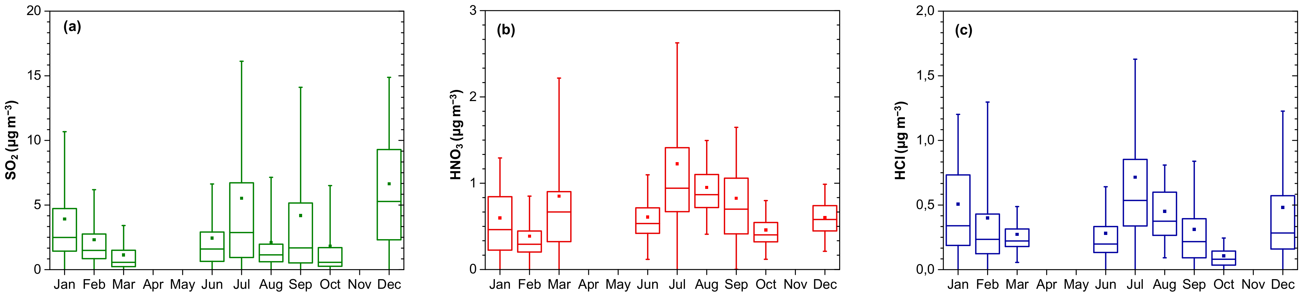
3.1.2. Seasonal Variability

The seasonal variability of SO₂ (Figure 3a) demonstrated higher mean levels in December relative to July by almost 20% (6.6 μg m⁻³ and 5.5 μg m⁻³, respectively). The increased SO₂ levels in the summer could be attributed to the absence of rain and the enhanced transport from the northern and northeastern sector (the Balkans, Russia, Ukraine, and Turkey), which is typical for this period of the year [77,78,79]. The winter maximum could be related to the increase in emissions by heating oil combustion, in combination with a lower mixing layer relative to the summer [80]. The proximity to local emission sources (especially heating) can further contribute to the observed seasonal profile, resulting in complex variability patterns compared to the observations for the coastal sites (e.g., a pronounced summer maximum for Finokalia, Crete [65], or for southern Europe [31]).

A pronounced seasonal pattern was observed for HNO₃ (Figure 3b), with a clear summer maximum and lower levels during the remaining months, as was also reported in previous works [51,52]. The average summer concentration of 0.9 μg m⁻³ was 70% higher than the winter one. The build-up of HNO₃ in the summer can be attributed to three processes: the increased abundance of OH radicals (

Table 2. Mean monthly 24 h levels of OH radicals based on the box-model simulations.

Month	OH × 106 Molecules cm−3
January	0.1 ± 0.2
February	0.2 ± 0.5
March	0.6 ± 1.2
June	1.6 ± 2.5
July	3.0 ± 4.7
August	3.6 ± 5.6
September	1.4 ± 2.9
October	1.1 ± 1.7
November	0.1 ± 0.2

) that react with NO₂; the absence of precipitation; and the increased volatility of particulate NH₄NO₃ under high temperatures that favors the formation of the gaseous HNO₃ (see also Section 3.3). An annual mean OH radical concentration equal to 1.5 ± 3.3 × 10⁶ molecules cm⁻³ was calculated in the area using the box model (Section 2.3). The summer OH radical levels were higher (2.7 × 10⁶ molecules cm⁻³). The mean concentration of 3.6 × 10⁶ molecules cm⁻³ in August (Table 2) falls within the range of the 24 h average concentrations of 3.6–6.7 × 10⁶ molecules cm⁻³ reported for Finokalia (Crete) during measurements performed in August 2001 (period mean: 4.5 ± 1.1 × 10⁶ molecules cm⁻³) [59]. Furthermore, the mean value of 3.0 × 10⁶ molecules cm⁻³ in July is also in good agreement with that reported in Cyprus for measurements performed in July 2014 (mean of 2.2 × 10⁶ molecules cm⁻³) [60]. The summer maximum for HNO₃ was in accordance with the seasonality reported by Tang et al. [31] for southern Europe. The HCl seasonal cycle (Figure 3c) follows that of the HNO₃, also displaying a summer peak, which could be linked with its production by the reaction of HNO₃ with sea salt, the absence of precipitation, and the volatilization of NH₄Cl.

3.1.3. Diurnal Variability

The mean diurnal cycles of acidic gas concentrations presented notable weekly and seasonal patterns (Figure 4). More precisely, for SO₂, a clear bimodal diurnal variability was observed and, taking into account the absence of significant local sources such as industries, the late-morning maximum (~1.5 times higher relative to the night one) (Figure 4a) could be linked to the development of the boundary layer and the intrusion of the long-range transported air masses. Vehicular emissions during the traffic rush hours or other local processes cannot be ruled out as a factor but are probably less important as the maximum weekdays–weekends difference at the 8:00–11:00 time frame was very small (10–20%). During the winter, an enhancement was observed for the nighttime levels of SO₂ (especially after 19:00 and until midnight) due to the shallower boundary layer and the emissions from heating (see also below; Figure 4b).

The average ratio of the daytime to nighttime peak concentrations for HNO₃ was above unity (~1.3) (Figure 4c), highlighting the importance of photochemistry in its formation (the mean OH radical concentration at noon on an annual basis was equal to 6.1 × 10⁶ molecules cm⁻³ according to the box-model simulations) and the volatilization of NH₄NO₃ during the warm hours of the day, in accordance with the observations of the seasonal trend. The diurnal variability of HCl (Figure 4e) was driven by the presence of HNO₃, thus displaying a similar pattern that is characterized, though, by an earlier afternoon enhancement. The HNO₃ levels were decreased during the weekends by almost 30% (Figure S2a) at noon, due to the limited availability of precursors, specifically NO₂ from vehicular emissions, especially during the summer (Figure S2b). Similar, but less pronounced, was the variability of HCl. When the diurnal variability is examined on a seasonal basis (summer vs. winter), higher noon maxima are observed in the summer for HNO₃ and HCl, highlighting the impact of photochemistry on HNO₃ formation and the further production of HCl (Figure 4d,f). HNO₃, especially, presented higher values in the summer relative to the winter (almost 3 times at 13:00), whereas for HCl, levels greater by 1.8 times were observed from 12:00 to 17:00. Conversely, for SO₂, the enhancement in the summer compared to the winter at noon was lower (less than 40%).

3.2. Evaluation of Factors Affecting the Levels of the Acidic Gases

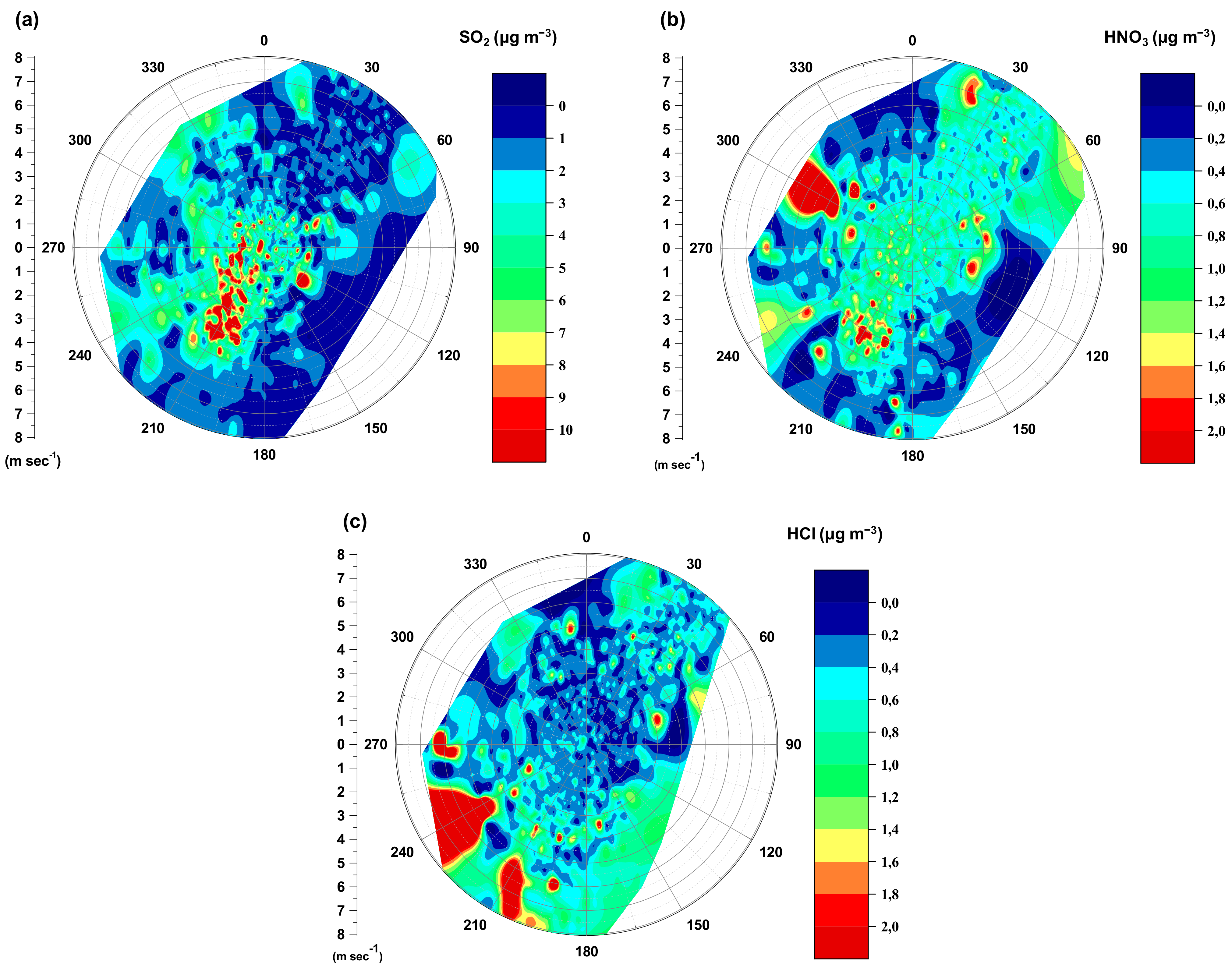
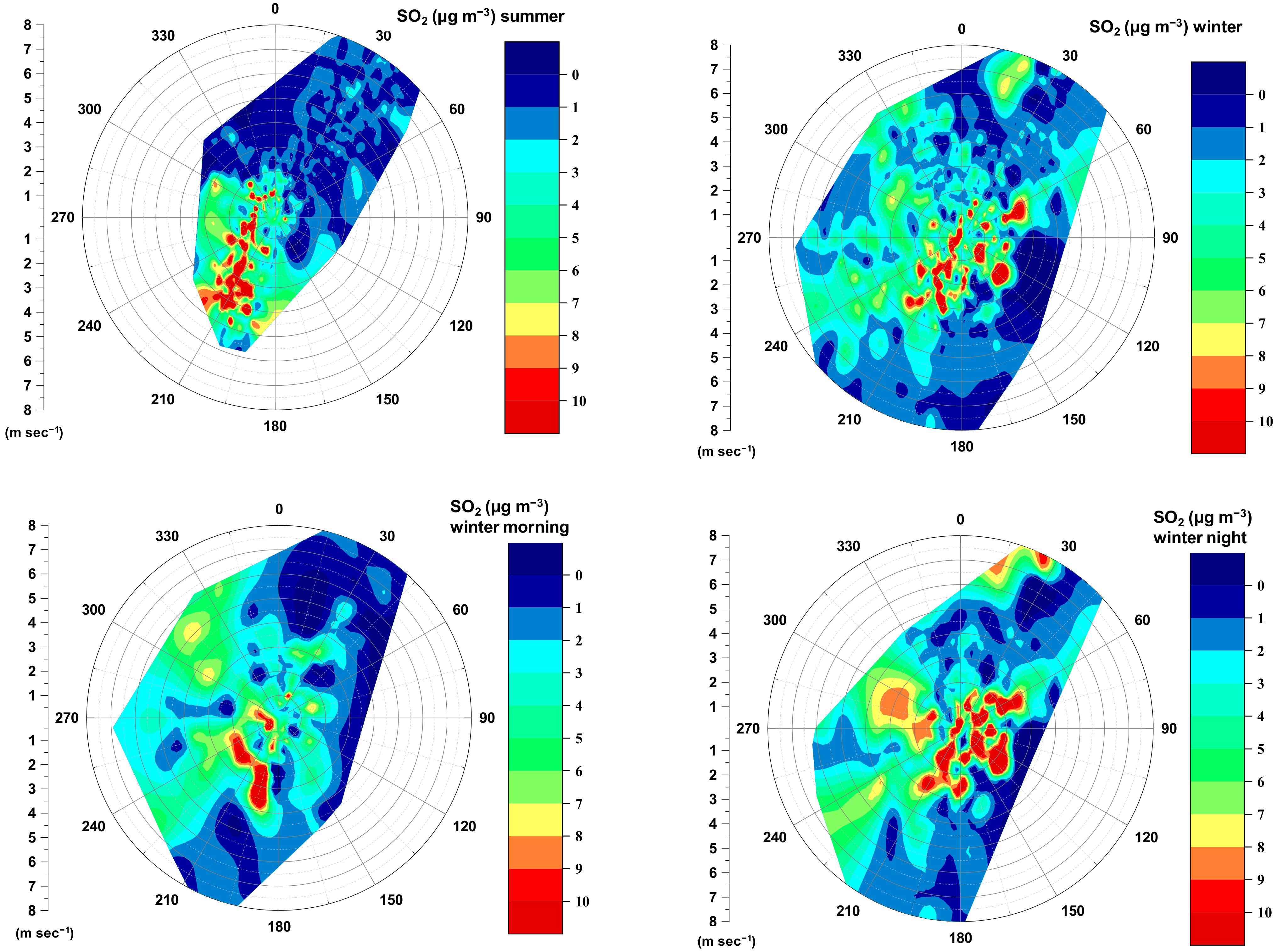
3.2.1. Role of Meteorology

The dependence of the SO₂ levels on wind speed and wind direction is depicted in Figure 5a. A mostly uniform distribution in the polar plot was observed, which reflects the regional character of SO₂. An enhancement was observed for the southwestern sector (210 ± 15°) for relatively intermediate wind speeds (2–4 m s⁻¹) and under low-wind conditions (<2 m s⁻¹) in all directions, which also indicates an impact from local emission sources, as was further confirmed in Figure S3a.

By investigating the wind dependence of SO₂ on a seasonal basis (Figure 6, upper row), differentiated patterns were observed, with the dominant emission sources during the summer being along the southwestern sector, which could be linked to shipping activities at the Piraeus Port in this direction [81], enhancing SO₂ levels at more than 8–9 μg m⁻³ relative to the northern sector that was characterized by low concentrations. In contrast, the maximum values in the winter were more or less equally distributed in the polar plot, with a slight enhancement for the southeastern–southwestern sector (Figure 6, upper row). As the heating needs in the winter are maximized in the night hours [37,38,82], morning and night polar plots were also considered. The time spans were selected based on the diurnal variability of the wood-burning and fossil-fuel fractions of black carbon (BC_wb and BC_ff, respectively). According to Liakakou et al. [54], the morning vehicular BC peak is observed between 7:00–11:00, whereas the combined impact of wood burning and fossil fuel attributed to both heating and traffic is expected from 18:00 to 02:00. During the winter mornings, SO₂ levels higher than 5 μg m⁻³ were encountered for all wind sectors, with stronger impacts under the S-SW winds of up to 100% (Figure 6, bottom row). Regarding BC, the wood-burning fraction had its lower levels and variability during morning, while a BC_ff enhancement was observed under northerly and easterly winds (Figure S4 left column), thus indicating that the SO₂ sources were not linked to traffic but rather to the intrusion of regional SO₂ during the gradual development of the boundary layer. During the night, the impact of the major processes regulating SO₂ levels, i.e., heating and traffic (Figure S4, right column) was more evident. Therefore, apart from the regional influence, the SO₂ emissions from local sources such as heating and shipping seem to hold a significant role in the atmospheric abundance of SO₂.

On the other hand, chemical transformations are expected to be more important for the levels of HNO₃ and HCl. The role of the local emission sources seems to be of secondary importance as no increase was observed under low winds as in the case of the SO₂ (Figure S3b,c). HNO₃ presented wind dependence (Figure 5b) similar to its precursor NO₂, at least on the small–medium spatial scale examined by the polar plots (Figure S5, bottom row). The role of photochemistry in the summer was reflected on a background of 0.4–0.8 μg m⁻³, relative to the dominance of levels <0.4μg m⁻³ in winter and obvious higher values of HNO₃ relative to the cold period, which was characterized by minimum OH radical levels (Figure S5, upper row, Table 2). The emission of HCl might occur from the coastal industrial area located at around 20 km west of the metropolitan area in the Thriassion plain. Simultaneously, production from the reaction of nitric acid with sodium chloride from sea spray is expected to play a significant role in the determination of the HCl levels. The contribution of both processes can be tracked in the HCl polar plot, with the maximum levels associated with winds from the marine sector (S, SW), regardless of the season (Figure 5c and Figure S5, middle row). In addition, the common characteristics of HCl with those of HNO₃ probably indicate the impact of heterogeneous reactions involving HNO₃ on the HCl production pathways.

3.2.2. Role of Emission Sources with Emphasis on Wood Burning

Apart from the meteorology, the emission sources, either local or regional, may also affect the levels of the acidic gases. Along with the significant correlations (r) of the acidic compounds with the gaseous and particulate indicators of the combustion processes (Table S1), a significant degree of covariance was also observed between SO₂ and HNO₃, indicating common emission sources. On the other hand, processes different to those of the traffic and heating seem to control HCl production. To assess the impact of the dominant emission sources in the GAA, and especially that of wood burning—which has exerted a significant impact on the atmospheric composition in Athens during the night in recent years [54]—

Table 3. Mean levels of acidic gases and tracers on various periods. The levels are given in μg m⁻³.

Average	SO2	HNO3	HCl	NO2	BC	BCwb	BCff
Winter	3.5 ± 4.1 (2.0)	0.5 ± 0.4 (0.4)	0.4 ± 0.6 (0.3)	25.2 ± 15.0 (20.6)	3.5 ± 4.4 (1.5)	1.7 ± 2.7 (0.6)	1.9 ± 2.3 (0.9)
Winter Day 1	3.2 ± 3.8 (1.9)	0.4 ± 0.3 (0.3)	0.4 ± 0.4 (0.3)	21.8 ± 12.7 (18.0)	2.4 ± 2.8 (1.3)	0.7 ± 0.9 (0.5)	1.7 ± 2.1 (0.8)
Winter Night 2	3.7 ± 4.3 (1.3)	0.5 ± 0.4 (0.4)	0.5 ± 0.6 (0.2)	28.7 ± 16.4 (25.9)	4.6 ± 5.3 (2.3)	2.7 ± 3.4 (1.2)	2.0 ± 2.4 (1.0)
Winter SP Night 3	5.4 ± 5.2 (3.6)	0.7 ± 0.4 (0.6)	0.3 ± 0.3 (0.2)	39.4 ± 14.5 (39.8)	7.1 ± 5.7 (5.1)	4.1 ± 3.7 (3.1)	3.1 ± 2.6 (2.3)
Winter nSP Night 4	1.9 ± 1.7 (1.3)	0.4 ± 0.3 (0.3)	0.6 ± 0.8 (0.3)	18.7 ± 10.9 (15.4)	1.1 ± 1.0 (0.9)	0.6 ± 0.8 (0.4)	0.6 ± 0.4 (0.5)
Dust	2.3 ± 2.8 (1.3)	0.6 ± 0.6 (0.4)	0.4 ± 0.5 (0.3)	24.9 ± 16.3 (18.9)	2.4 ± 3.1 (1.2)	0.8 ± 1.7 (0.2)	1.7 ± 1.8 (0.9)
no Dust	3.6 ± 5.3 (1.7)	0.8 ± 0.6 (0.7)	0.4 ± 0.4 (0.3)	23.2 ± 15.6 (17.1)	2.0 ± 2.8 (1.1)	0.6 ± 1.6 (0.2)	1.4 ± 1.6 (0.9)

¹ 6:00–17:00; ² 18:00–5:00; ³ 18:00–5:00 and SP; ⁴ 18:00–5:00; and nSP.

presents the concentration statistics for the acidic compounds during selected periods. The start times of the day and night periods were defined as 6:00 and 18:00, respectively. The nighttime data obtained during the winter were further classified into smog and non-smog periods (SP and nSP, respectively), taking into account in the definition of an SP period the combination of low wind speed and the absence of precipitation [37] that enhance the accumulation of the pollutants. Furthermore, the presence of transported dust was also considered on an annual basis, as the dust can react with the acidic species studied here. The impact of heating emissions during the smog events was obvious in the SO₂ levels as they increased by almost 3 and 2 times relative to the levels during the non-smog periods and the daytime, respectively. Less significant, but still important, was the impact on the HNO₃ nighttime concentrations, as they increased by 50%. HCl presented an opposite trend, with higher levels during the non-smog periods, supporting production by heterogeneous reactions of gaseous HNO₃ with sodium chloride (NaCl) from transported sea salt particles [77] under favorable conditions, i.e., dominance of marine air masses and increased wind speed.

Moreover, when dust is present it has an important role in the determination of the SO₂ and HNO₃ levels, acting as a clear sink and reducing them by almost 40% (Table 3). The above result is in excellent agreement with Kocak et al. [83], who reported an enhancement in sulfate and nitrate aerosols during dust events in the Eastern Mediterranean. It is also supported by other field and laboratory studies indicating that mineral dust particles can serve as reaction surfaces for different species, including SO₂, N₂O₅, and HNO₃ [84,85]. For HCl, the absence of any significant change could probably indicate a competition between HCl adsorption on dust and HCl production from the reaction of HNO₃ with sea salt as dust intrusions, in the vast majority of cases, originate from the south (i.e., from the marine sector).

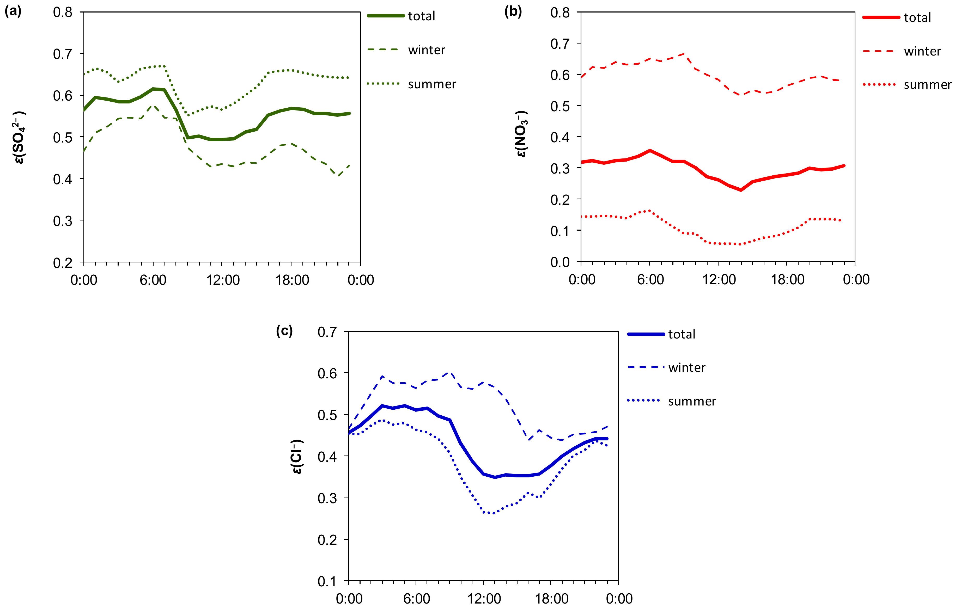
3.3. Phase Distribution of the Gaseous Aerosol Precursors

For the greater part of the measurement period, the simultaneous monitoring of submicron (PM₁) water-soluble anions took place using a PILS-IC instrument. Table S2 presents the monthly mean values (arithmetic mean and standard deviation) of the aforementioned species. As also reported by works conducted in the GAA and the Eastern Mediterranean in general, the SO₄²⁻ levels maximized here in the summer (maximum at 7.7 μg m⁻³ in July) due to the increased photochemical activity and the limited wet deposition that favors the long-range transport of aerosols [65,79,86,87]. Therefore, sulfate followed the seasonal variability of SO₂. On the other hand, increased winter levels (1.2 μg m⁻³ versus lower than 0.1 μg m⁻³ in the summer) were observed for the NO₃⁻, a trend opposite to that observed for the HNO₃. Finally, Cl⁻ did not exhibit noteworthy seasonal variation, with mean values not exceeding 0.3 μg m⁻³ per season. Ammonium nitrate stabilizes under the low temperatures prevailing in the winter, leading to increased NO₃⁻ levels [88,89]. Additionally, enhanced local pollution sources, such as residential heating, could also contribute to the increased NO₃⁻ levels observed during the night, in agreement with the results reported for the GAA using filter-based and near-real-time techniques [40,90,91]. The diurnal variability of sulfate was mainly driven by the development of the boundary layer from early morning until noon (Figure S6a). In the case of NO₃⁻, the main drivers of the diurnal variability were the stabilization of ammonium nitrate (maximized during the night) and the boundary-layer variability (minimized during the night; Figure S6b). Finally, no significant diurnal variability was observed for chloride as it is expected to be mostly linked to sea salt particles (Figure S6c).

Computation of the partitioning ratios (ε; particulate/particulate + gaseous) of the pairs SO₄²⁻-SO₂, NO₃⁻-HNO₃, and Cl⁻-HCl, i.e., the particles and corresponding inorganic gases, can provide useful information on the prevailing forms of the compounds. This information is very important as it is directly related to the lifetimes of the species of interest. For instance, the lifetimes of the submicron S-, N-, and Cl-containing particles are in the order of one week, much higher than when compared to their precursors in the gas phase, which allows them to travel much longer distances and thus to impact the atmospheric chemistry and/or the productivity of ecosystems (for example, N is a very important nutrient). Consequently, the partitioning ratios were calculated when measurements for both types of species were available, and the results are presented in Table S2. The average partitioning ratios for the submicron fraction were as follows: ε (SO₄²⁻) = 56 ± 20%, ε (NO₃⁻) = 30 ± 25%, and ε (Cl⁻) = 44 ± 23%. Measurements of partitioning ratios are very scarce in the literature. For instance, during May–June 2010 in Pasadena, CA, values of PM₁ ε(NO₃⁻) = 39 ± 16% and PM_2.5 ε(Cl⁻) = 39 ± 26% were reported for a coastal urban site impacted by high levels of sea salt aerosol, total nitrate, and ammonia [92]. These values were two times higher and 50% lower relative to the present values for June 2015 (ε (NO₃⁻) = 19 ± 10% and ε (Cl⁻) = 55 ± 21%, respectively), indicating an important site-to-site variability.

Of great importance is the diurnal variability of the partitioning ratios presented in Figure 7a–c. For SO₂, the particulate phase was calculated to be dominant during the summer, whereas during the winter both phases seemed to contribute equally. In both cases, a minimum is observed at noon, indicating the probable entrainment of SO₂ during the development of the BL, with the mean noon minimum to maximum ε (SO₄²⁻) not varying more than 30% (Figure 7a).

The HNO₃ and HCl presented a pattern opposite to the SO₂, with an enhancement of the particulate phase in winter. Especially in the case of nitrogen (N), pronounced differences were observed for ε (NO₃⁻), with the mean winter and summer values being equal to 60% and 11%, respectively (Figure 7b). For the HCl, the winter/summer ratio was smaller (by a factor of 2 or less; see Table S2) but still of note. As both HNO₃ and HCl are acids, aerosol pH should play an important role in determining their gas/particulate partition [93]. Indeed, in a study conducted during the summer at the remote site of Finokalia (Crete), under the strong impact of air masses from biomass burning (BB), Bougiatioti et al. [94] reported an increase in aerosol pH from 1.30 (an impact of the continental Europe air masses) to 2.77 ± 0.88. Given that biomass burning prevails in the GAA during the winter, a pH > 2 is expected during the cold period that could approach or surpass the estimations of 2.77 [95]. Such pH changes can significantly impact the partition of the nitrate ion and explain the observed summer/winter difference as well as the diurnal variation [70]. Similarly, pH changes can also explain HCl behavior, although the characterization of the effect should be more complicated as HCl formation depends not only on the levels of HNO₃ available in the gaseous phase but also on the amount of chloride from sea salt, which in turn depends on wind circulation.

4. Conclusions

The acidic gases HNO₃, HCl, and SO₂, apart from being the precursors of key aerosol species, also contribute to air quality, the oxidative potential of the atmosphere, and ecosystem productivity. In the current work, by using high-resolution techniques, we reported the levels, variability, and phase partitioning of the HNO₃, HCl, and SO₂ in Athens, Greece, over the period of 2014–2016.

High-resolution measurements of these compounds, and especially of HNO₃ and HCl, are extremely scarce in the Eastern Mediterranean and are reported here for the first time in Greece. Additionally, our database is the longest reported for the Eastern Mediterranean. Finally, it is worth noting that the most recent measurements of HNO₃ and HCl in Athens were reported 20 years ago. Since then, significant changes have occurred in the air quality, with important pollution abetment strategies, including deindustrialization, but also with the appearance of a new source related to residential wood burning (after 2012 and up to this day). Thus, the present work brings new data which are useful not only for the modelers but also for the policy makers. Finally, gas-to-particle partitioning for the studied compounds was also reported for the first time, to our knowledge, for the Eastern Mediterranean. This information is very important as it is directly related to the lifetimes of the species of interest, which in turn impact the atmospheric chemistry and/or the productivity of the ecosystems.

The measurements were conducted at the urban background Thissio Air Monitoring Station of the National Observatory of Athens and cover periods typical of the cold and warm conditions, as well as the transition seasons. The aim was to assess the impact of the meteorology and emission sources on their levels, on a diurnal and seasonal basis. A wet annular denuder system paired with an ion chromatograph was operated, facilitating the almost near-real-time monitoring of the acidic gases, whereas auxiliary measurements of water-soluble anions and combustion tracers, as well as modeling simulations, supported the analysis.

The application of emission-abatement policies and pollution-control technologies over the last 20 years was reflected in the mean levels of SO₂ and HNO₃ relative to the reported values of the past in Athens. On the other hand, as the records for HCl are scarce, no firm conclusion can be drawn on its long-term trend. Regarding the seasonal variability, the mean SO₂ levels presented both winter and summer maxima. In the winter, the enhanced levels were due to the increased emissions from heating combined with the low boundary layer and the absence of rainfall, while the summer maxima were mostly due to aerosol transport. The intrusion of regional SO₂ was responsible for the noon maximum observed in the diurnal cycles, whereas the vehicular emissions did not significantly affect the SO₂ levels. The impact of local sources on the SO₂ was clearly reflected by the enhancement of its levels observed under low wind speeds (<3 m s⁻¹). The southern sector that includes the Piraeus Port was the main local source, especially in the summer, and was possibly linked to shipping activities. On the other hand, residential heating proved to be the most important local source of SO₂ during the winter nights.

As opposed to the SO₂, a clear build-up of HNO₃ was observed in the summer (0.9 μg m⁻³ versus 0.5 μg m⁻³ for the cold period). This seasonality resulted from the increased photochemical activity (average daily OH concentration of ~2.7 × 10⁶ molecules cm⁻³; an order of magnitude higher in the summer compared to the winter), the absence of precipitation, and the increased volatilization and dissociation of the particulate NH₄NO₃ back to HNO₃, under the high temperatures occurring in summer. The role of photochemistry was also obvious on the diurnal variability, leading to 30% higher levels during the day relative to the night, while during the weekends, the lower levels of NO₂ led to HNO₃ levels decreased by 30%. The similarities between the HCl and HNO₃ seasonal variabilities were attributed to HCl production by the heterogeneous reactions of HNO₃ on sea salt, the absence of precipitation, and the volatilization and dissociation of NH₄Cl to HCl. Furthermore, the noon levels of HCl were almost doubled in the summer compared to the winter, following the HNO₃ trend.

Although traffic remains one of the major emission sources in Athens, the recession after 2008 and the changes in fuels used for heating purposes resulted in biomass burning being currently the prevalent source during winter. The presence of smog events during winter nights enhanced the levels of SO₂ and HNO₃ by almost 300% and 50% relative to the conditions that favor the dispersion of pollutants, thus highlighting the strength of this source and its impacts on air quality. On the other hand, the production of HCl was favored during days without smog events, supporting its formation by the heterogeneous reactions of gaseous HNO₃ with sodium chloride (NaCl) on sea salt particles present in central Athens under stronger winds. The latter production pathway of HCl competes with the adsorption on particles during dust events, leading finally to almost similar levels of about 0.4 μg m⁻³ during, and in the absence of, dust events. Conversely, the reduction in SO₂ and HNO₃ levels by 40% during dust events highlights the role of dust as a sink for these compounds.

The partition of the studied compounds on the particulate or gaseous phase was assessed by the partitioning ratios (ε). The mean ε (SO₄²⁻) = 56 ± 20%, ε (NO₃⁻) = 30 ± 25%, and ε (Cl⁻) = 44 ± 23% deviated from the published values in the US, indicating important site-to-site variability. For SO₂, the particulate phase was calculated to be the dominant one during the summer, whereas during the winter both phases contributed equally. A contrasted behavior was seen for HNO₃ and HCl as the particulate phase dominated in the winter with mean ε (NO₃⁻) = 60%. The important winter/summer difference could be linked to aerosol acidity. Indeed, the biomass-burning emitted compounds are anticipated to increase significantly in pH to values of up to 2.8, as has been observed at the remote coastal site of Finokalia in Crete. Considering the strength of smog events in the GAA during the winter, similar pH values are also expected in the GAA during the winter. Such nitrate partitioning at the particulate phase can affect the transport of fine particles far from the emission sources, contributing to the acidification of ecosystems and/or the decay of building materials, highlighting the importance of the current work and advocating for future specialized research on the topic.

References

1. Kitto, A.M.N.; Harrison, R.M. Nitrous and nitric acid measurements at sites in South-East England. Atmos. Environ. Part A Gen. Top. 1992, 26, 235–241. [Google Scholar] [CrossRef]
2. Atkinson, R.; Baulch, D.L.; Cox, R.A.; Crowley, J.N.; Hampson, R.F.; Haynes, R.G.; Jenkin, M.E.; Rossi, M.J.; Troe, J. Evaluated kinetic and photochemical data for atmospheric chemistry: Volume I-Gas phase reactions of Ox, HOx, NOx and SOx species. Atmos. Chem. Phys. 2004, 4, 1461–1738. [Google Scholar] [CrossRef] [Green Version]
3. Heintz, F.; Platt, U.; Flentje, H.; Dubois, R. Long-term observation of nitrate radicals at the Tor Station, Kap Arkona (Rügen). J. Geophys. Res. Atmos. 1996, 101, 22891–22910. [Google Scholar] [CrossRef]
4. Dai, M.; Yu, Z.; Tang, Y.; Ma, X. HCl emission and capture characteristics during PVC and food waste combustion in CO2/O2 atmosphere. J. Energy Inst. 2020, 93, 1036–1044. [Google Scholar] [CrossRef]
5. Zhang, H.; Yu, S.; Shao, L.; He, P. Estimating source strengths of HCl and SO2 emissions in the flue gas from waste incineration. J. Environ. Sci. 2019, 75, 370–377. [Google Scholar] [CrossRef]
6. Eldering, A.; Solomon, P.A.; Salmon, L.G.; Fall, T.; Cass, G.R. Hydrochloric acid: A regional perspective on concentrations and formation in the atmosphere of Southern California. Atmos. Environ. Part A Gen. Top. 1991, 25, 2091–2102. [Google Scholar] [CrossRef]
7. Crisp, T.A.; Lerner, B.M.; Williams, E.J.; Quinn, P.K.; Bates, T.S.; Bertram, T.H. Observations of gas phase hydrochloric acid in the polluted marine boundary layer. J. Geophys. Res. 2014, 119, 6897–6915. [Google Scholar] [CrossRef]
8. Berresheim, H.; Jaeschke, W. The contribution of volcanoes to the global atmospheric sulfur budget. J. Geophys. Res. 1983, 88, 3732–3740. [Google Scholar] [CrossRef]
9. Erisman, J.W.; Bleeker, A.; Galloway, J.; Sutton, M.S. Reduced nitrogen in ecology and the environment. Environ. Pollut. 2007, 150, 140–149. [Google Scholar] [CrossRef] [Green Version]
10. Sutton, M.A.; Dragosits, U.; Tang, Y.S.; Fowler, D. Ammonia emissions from non-agricultural sources in the UK. Atmos. Environ. 2000, 34, 855–869. [Google Scholar] [CrossRef]
11. Zhao, B.; Wang, P.; Ma, J.Z.; Zhu, S.; Pozzer, A.; Li, W. A high-resolution emission inventory of primary pollutants for the Huabei region, China. Atmos. Chem. Phys. 2012, 12, 481–501. [Google Scholar] [CrossRef] [Green Version]
12. Tsimpidi, A.P.; Karydis, V.A.; Pandis, S.N. Response of inorganic fine particulate matter to emission changes of sulfur dioxide and ammonia: The Eastern United States as a case study. J. Air Waste Manag. Assoc. 2007, 57, 1489–1498. [Google Scholar] [CrossRef]
13. Pye, H.O.T.; Nenes, A.; Alexander, B.; Ault, A.P.; Barth, M.C.; Clegg, S.L.; Collett, J.L.; Fahey, K.M.; Hennigan, C.J.; Herrmann, H.; et al. The acidity of atmospheric particles and clouds. Atmos. Chem. Phys. 2020, 20, 4809–4888. [Google Scholar] [CrossRef] [Green Version]
14. Freedman, M.A.; Ott, E.-J.E.; Marak, K.E. Role of pH in Aerosol Processes and Measurement Challenges. J. Phys. Chem. A 2019, 123, 1275–1284. [Google Scholar] [CrossRef] [Green Version]
15. Stockdale, A.; Krom, M.D.; Mortimer, R.J.G.; Benning, L.G.; Carslaw, K.S.; Herbert, R.J.; Shi, Z.; Myriokefalitakis, S.; Kanakidou, M.; Nenes, A. Understanding the nature of atmospheric acid processing of mineral dusts in supplying bioavailable phosphorus to the oceans. Proc. Natl. Acad. Sci. USA 2016, 113, 14639–14644. [Google Scholar] [CrossRef] [Green Version]
16. Weber, R.J.; Guo, H.; Russell, A.G.; Nenes, A. High aerosol acidity despite declining atmospheric sulfate concentrations over the past 15 years. Nat. Geosci. 2016, 9, 282–285. [Google Scholar] [CrossRef]
17. Lelieveld, J.; Evans, J.S.; Fnais, M.; Giannadaki, D.; Pozzer, A. The contribution of outdoor air pollution sources to premature mortality on a global scale. Nature 2015, 525, 367–371. [Google Scholar] [CrossRef]
18. Benedict, K.B.; Day, D.; Schwandner, F.M.; Kreidenweis, S.M.; Schichtel, B.; Malm, W.C.; Collett, J.L. Observations of atmospheric reactive nitrogen species in Rocky Mountain National Park and across northern Colorado. Atmos. Environ. 2013, 64, 66–76. [Google Scholar] [CrossRef]
19. Chen, X.; Walker, J.T.; Geron, C. Chromatography related performance of the Monitor for AeRosols and GAses in ambient air (MARGA): Laboratory and field-based evaluation. Atmos. Meas. Tech. 2017, 10, 3893–3908. [Google Scholar] [CrossRef] [Green Version]
20. Hsu, Y.M.; Clair, T.A. Measurement of fine particulate matter water-soluble inorganic species and precursor gases in the Alberta oil sands region using an improved semicontinuous monitor. J. Air Waste Manag. Assoc. 2015, 65, 423–435. [Google Scholar] [CrossRef] [Green Version]
21. Le, T.C.; Wang, Y.C.; Pui, D.Y.H.; Tsai, C.J. Characterization of atmospheric PM2.5 inorganic aerosols using the semi-continuous PPWD-PILS-IC system and the ISORROPIA-II. Atmosphere 2020, 11, 820. [Google Scholar] [CrossRef]
22. Li, Z.; Liu, Y.; Lin, Y.; Gautam, S.; Kuo, H.C.; Tsai, C.J.; Yeh, H.; Huang, W.; Li, S.W.; Wu, G.J. Development of an automated system (PPWD/PILS) for studying PM2.5 water-soluble ions and precursor gases: Field measurements in two cities, Taiwan. Aerosol Air Qual. Res. 2017, 17, 426–443. [Google Scholar] [CrossRef] [Green Version]
23. Markovic, M.Z.; Vandenboer, T.C.; Murphy, J.G. Characterization and optimization of an online system for the simultaneous measurement of atmospheric water-soluble constituents in the gas and particle phases. J. Environ. Monit. 2012, 14, 1872–1884. [Google Scholar] [CrossRef] [PubMed]
24. Nie, W.; Wang, T.; Gao, X.; Pathak, R.K.; Wang, X.; Gao, R.; Zhang, Q.; Yang, L.; Wang, W. Comparison among filter-based, impactor-based and continuous techniques for measuring atmospheric fine sulfate and nitrate. Atmos. Environ. 2010, 44, 4396–4403. [Google Scholar] [CrossRef]
25. Ten Brink, H.; Otjes, R.; Jongejan, P.; Slanina, S. An instrument for semi-continuous monitoring of the size-distribution of nitrate, ammonium, sulphate and chloride in aerosol. Atmos. Environ. 2007, 41, 2768–2779. [Google Scholar] [CrossRef] [Green Version]
26. Rumsey, I.C.; Cowen, K.A.; Walker, J.T.; Kelly, T.J.; Hanft, E.A.; Mishoe, K.; Rogers, C.; Proost, R.; Beachley, G.M.; Lear, G.; et al. An assessment of the performance of the Monitor for AeRosols and GAses in ambient air (MARGA): A semi-continuous method for soluble compounds. Atmos. Chem. Phys. 2014, 14, 5639–5658. [Google Scholar] [CrossRef] [Green Version]
27. Trebs, I.; Meixner, F.X.; Slanina, J.; Otjes, R.; Jongejan, P.; Andreae, M.O. Real-time measurements of ammonia, acidic trace gases and water-soluble inorganic aerosol species at a rural site in the Amazon Basin. Atmos. Chem. Phys. 2004, 4, 967–987. [Google Scholar] [CrossRef] [Green Version]
28. Xu, Z.; Liu, Y.; Nie, W.; Sun, P.; Chi, X.; Ding, A. Evaluating the measurement interference of wet rotating-denuder-ion chromatography in measuring atmospheric HONO in a highly polluted area. Atmos. Meas. Tech. 2019, 12, 6737–6748. [Google Scholar] [CrossRef] [Green Version]
29. EMEP. Air Pollution Trends in the EMEP Region between 1990 and 2012; NILU: Kjeller, Norway, 2016. [Google Scholar]
30. European Environment Agency (EEA). Air Quality in Europe-2020 Report; Publications Office of the European Union: Luxembourg, 2020; ISBN 978-92-9480-292-7. [Google Scholar]
31. Tang, Y.S.; Flechard, C.R.; Dämmgen, U.; Vidic, S.; Djuricic, V.; Mitosinkova, M.; Uggerud, H.T.; Sanz, M.J.; Simmons, I.; Dragosits, U.; et al. Pan-European rural monitoring network shows dominance of NH3 gas and NH4NO3 aerosol in inorganic atmospheric pollution load. Atmos. Chem. Phys. 2021, 21, 875–914. [Google Scholar] [CrossRef]
32. Roig Rodelas, R.; Perdrix, E.; Herbin, B.; Riffault, V. Characterization and variability of inorganic aerosols and their gaseous precursors at a suburban site in northern France over one year (2015–2016). Atmos. Environ. 2019, 200, 142–157. [Google Scholar] [CrossRef]
33. Metzger, S.; Mihalopoulos, N.; Lelieveld, J. Importance of mineral cations and organics in gas-aerosol partitioning of reactive nitrogen compounds: Case study based on MINOS results. Atmos. Chem. Phys. 2006, 6, 2549–2567. [Google Scholar] [CrossRef] [Green Version]
34. Hanke, M.; Umann, B.; Uecker, J.; Arnold, F.; Bunz, H. Atmospheric measurements of gas-phase HNO3 and SO2 using chemical ionization mass spectrometry during the MINATROC field campaign 2000 on Monte Cimone. Atmos. Chem. Phys. 2003, 3, 417–436. [Google Scholar] [CrossRef] [Green Version]
35. Makkonen, U.; Virkkula, A.; Mäntykenttä, J.; Hakola, H.; Keronen, P.; Vakkari, V.; Aalto, P.P. Semi-continuous gas and inorganic aerosol measurements at a Finnish urban site: Comparisons with filters, nitrogen in aerosol and gas phases, and aerosol acidity. Atmos. Chem. Phys. 2012, 12, 5617–5631. [Google Scholar] [CrossRef] [Green Version]
36. Stieger, B.; Spindler, G.; Fahlbusch, B.; Müller, K.; Grüner, A.; Poulain, L.; Thöni, L.; Seitler, E.; Wallasch, M.; Herrmann, H. Measurements of PM10 ions and trace gases with the online system MARGA at the research station Melpitz in Germany–A five-year study. J. Atmos. Chem. 2018, 75, 33–70. [Google Scholar] [CrossRef]
37. Fourtziou, L.; Liakakou, E.; Stavroulas, I.; Theodosi, C.; Zarmpas, P.; Psiloglou, B.; Sciare, J.; Maggos, T.; Bairachtari, K.; Bougiatioti, A.; et al. Multi-tracer approach to characterize domestic wood burning in Athens (Greece) during wintertime. Atmos. Environ. 2017, 148, 89–101. [Google Scholar] [CrossRef]
38. Gratsea, M.; Liakakou, E.; Mihalopoulos, N.; Adamopoulos, A.; Tsilibari, E.; Gerasopoulos, E. The combined effect of reduced fossil fuel consumption and increasing biomass combustion on Athens’ air quality, as inferred from long term CO measurements. Sci. Total Environ. 2017, 592, 115–123. [Google Scholar] [CrossRef]
39. Kalogridis, A.-C.; Vratolis, S.; Liakakou, E.; Gerasopoulos, E.; Mihalopoulos, N.; Eleftheriadis, K. Assessment of wood burning versus fossil fuel contribution to wintertime black carbon and carbon monoxide concentrations in Athens, Greece. Atmos. Chem. Phys. 2018, 18, 10219–10236. [Google Scholar] [CrossRef] [Green Version]
40. Theodosi, C.; Tsagkaraki, M.; Zarmpas, P.; Grivas, G.; Liakakou, E.; Paraskevopoulou, D.; Lianou, M.; Gerasopoulos, E.; Mihalopoulos, N. Multi-year chemical composition of the fine-aerosol fraction in Athens, Greece, with emphasis on the contribution of residential heating in wintertime. Atmos. Chem. Phys. 2018, 18, 14371–14391. [Google Scholar] [CrossRef] [Green Version]
41. Grivas, G.; Stavroulas, I.; Liakakou, E.; Kaskaoutis, D.G.; Bougiatioti, A.; Paraskevopoulou, D.; Gerasopoulos, E.; Mihalopoulos, N. Measuring the spatial variability of black carbon in Athens during wintertime. Air Qual. Atmos. Health 2019, 12, 1405–1417. [Google Scholar] [CrossRef]
42. Katsanos, D.; Bougiatioti, A.; Liakakou, E.; Kaskaoutis, D.G.; Stavroulas, I.; Paraskevopoulou, D.; Lianou, M.; Psiloglou, B.E.; Gerasopoulos, E.; Pilinis, C.; et al. Optical properties of near-surface urban aerosols and their chemical tracing in a mediterranean city (Athens). Aerosol Air Qual. Res. 2019, 19, 49–70. [Google Scholar] [CrossRef]
43. Panopoulou, A.; Liakakou, E.; Gros, V.; Sauvage, S.; Locoge, N.; Bonsang, B.; Psiloglou, B.E.; Gerasopoulos, E.; Mihalopoulos, N. Non-methane hydrocarbon variability in Athens during wintertime: The role of traffic and heating. Atmos. Chem. Phys. 2018, 18, 16139–16154. [Google Scholar] [CrossRef] [Green Version]
44. Hellén, H.; Tykkä, T.; Hakola, H. Importance of monoterpenes and isoprene in urban air in northern Europe. Atmos. Environ. 2012, 59, 59–66. [Google Scholar] [CrossRef]
45. Panopoulou, A.; Liakakou, E.; Sauvage, S.; Gros, V.; Locoge, N.; Stavroulas, I.; Bonsang, B.; Gerasopoulos, E.; Mihalopoulos, N. Yearlong measurements of monoterpenes and isoprene in a Mediterranean city (Athens): Natural vs. anthropogenic origin. Atmos. Environ. 2020, 243, 117803. [Google Scholar] [CrossRef]
46. Panopoulou, A.; Liakakou, E.; Sauvage, S.; Gros, V.; Locoge, N.; Bonsang, B.; Salameh, T.; Gerasopoulos, E.; Mihalopoulos, N. Variability and sources of non-methane hydrocarbons at a Mediterranean urban atmosphere: The role of biomass burning and traffic emissions. Sci. Total Environ. 2021, 800, 149389. [Google Scholar] [CrossRef] [PubMed]
47. Orsini, D.A.; Ma, Y.; Sullivan, A.; Sierau, B.; Baumann, K.; Weber, R.J. Refinements to the particle-into-liquid sampler (PILS) for ground and airborne measurements of water soluble aerosol composition. Atmos. Environ. 2003, 37, 1243–1259. [Google Scholar] [CrossRef]
48. Weber, R.J.; Orsini, D.; Daun, Y.; Lee, Y.N.; Klotz, P.J.; Brechtel, F. A particle-into-liquid collector for rapid measurement of aerosol bulk chemical composition. Aerosol Sci. Technol. 2001, 35, 718–727. [Google Scholar] [CrossRef] [Green Version]
49. Sciare, J.; D’Argouges, O.; Sarda-Estève, R.; Gaimoz, C.; Dolgorouky, C.; Bonnaire, N.; Favez, O.; Bonsang, B.; Gros, V. Large contribution of water-insoluble secondary organic aerosols in the region of Paris (France) during wintertime. J. Geophys. Res. Atmos. 2011, 116, D22203. [Google Scholar] [CrossRef] [Green Version]
50. Collaud Coen, M.; Weingartner, E.; Apituley, A.; Ceburnis, D.; Fierz-Schmidhauser, R.; Flentje, H.; Henzing, J.S.; Jennings, S.G.; Moerman, M.; Petzold, A.; et al. Minimizing light absorption measurement artifacts of the Aethalometer: Evaluation of five correction algorithms. Atmos. Meas. Tech. 2010, 3, 457–474. [Google Scholar] [CrossRef] [Green Version]
51. Weingartner, E.; Saathoff, H.; Schnaiter, M.; Streit, N.; Bitnar, B.; Baltensperger, U. Absorption of light by soot particles: Determination of the absorption coefficient by means of aethalometers. J. Aerosol Sci. 2003, 34, 1445–1463. [Google Scholar] [CrossRef]
52. Sandradewi, J.; Prévôt, A.S.H.; Szidat, S.; Perron, N.; Alfarra, M.R.; Lanz, V.A.; Weingartner, E.; Baltensperger, U. Using aerosol light absorption measurements for the quantitative determination of wood burning and traffic emission contributions to particulate matter. Environ. Sci. Technol. 2008, 42, 3316–3323. [Google Scholar] [CrossRef]
53. Drinovec, L.; Močnik, G.; Zotter, P.; Prévôt, A.S.H.; Ruckstuhl, C.; Coz, E.; Rupakheti, M.; Sciare, J.; Müller, T.; Wiedensohler, A.; et al. The “dual-spot” Aethalometer: An improved measurement of aerosol black carbon with real-time loading compensation. Atmos. Meas. Tech. 2015, 8, 1965–1979. [Google Scholar] [CrossRef] [Green Version]
54. Liakakou, E.; Stavroulas, I.; Kaskaoutis, D.G.; Grivas, G.; Paraskevopoulou, D.; Dumka, U.C.; Tsagkaraki, M.; Bougiatioti, A.; Oikonomou, K.; Sciare, J.; et al. Long-term variability, source apportionment and spectral properties of black carbon at an urban background site in Athens, Greece. Atmos. Environ. 2020, 222, 117137. [Google Scholar] [CrossRef]
55. Dimitriou, K.; Liakakou, E.; Lianou, M.; Psiloglou, B.; Kassomenos, P.; Mihalopoulos, N.; Gerasopoulos, E. Implementation of an aggregate index to elucidate the influence of atmospheric synoptic conditions on air quality in Athens, Greece. Air Qual. Atmos. Health 2020, 13, 447–458. [Google Scholar] [CrossRef]
56. Stein, A.F.; Draxler, R.R.; Rolph, G.D.; Stunder, B.J.B.; Cohen, M.D.; Ngan, F. NOAA’s HYSPLIT atmospheric transport and dispersion modeling system. Bull. Am. Meteorol. Soc. 2015, 96, 2059–2077. [Google Scholar] [CrossRef]
57. Myriokefalitakis, S.; Daskalakis, N.; Gkouvousis, A.; Hilboll, A.; Van Noije, T.; Williams, J.E.; Le Sager, P.; Huijnen, V.; Houweling, S.; Bergman, T.; et al. Description and evaluation of a detailed gas-phase chemistry scheme in the TM5-MP global chemistry transport model (r112). Geosci. Model Dev. 2020, 13, 5507–5548. [Google Scholar] [CrossRef]
58. Myriokefalitakis, S.; Bergas-Massó, E.; Gonçalves-Ageitos, M.; Pérez García-Pando, C.; Van Noije, T.; Le Sager, P.; Ito, A.; Athanasopoulou, E.; Nenes, A.; Kanakidou, M.; et al. Multiphase processes in the EC-Earth Earth System model and their relevance to the atmospheric oxalate, sulfate, and iron cycles. Geosci. Model Dev. Discuss. in review. 2021. [Google Scholar] [CrossRef]
59. Dee, D.P.; Uppala, S.M.; Simmons, A.J.; Berrisford, P.; Poli, P.; Kobayashi, S.; Andrae, U.; Balmaseda, M.A.; Balsamo, G.; Bauer, P.; et al. The ERA-Interim reanalysis: Configuration and performance of the data assimilation system. Q. J. R. Meteorol. Soc. 2011, 137, 553–597. [Google Scholar] [CrossRef]
60. Williams, J.E.; Folkert Boersma, K.; Le Sager, P.; Verstraeten, W.W. The high-resolution version of TM5-MP for optimized satellite retrievals: Description and validation. Geosci. Model Dev. 2017, 10, 721–750. [Google Scholar] [CrossRef] [Green Version]
61. Damian, V.; Sandu, A.; Damian, M.; Potra, F.; Carmichael, G.R. The kinetic preprocessor KPP-A software environment for solving chemical kinetics. Comput. Chem. Eng. 2002, 26, 1567–1579. [Google Scholar] [CrossRef]
62. Sandu, A.; Sander, R. Technical note: Simulating chemical systems in Fortran90 and Matlab with the Kinetic PreProcessor KPP-2.1. Atmos. Chem. Phys. 2006, 6, 187–195. [Google Scholar] [CrossRef] [Green Version]
63. Sander, R.; Baumgaertner, A.; Cabrera-Perez, D.; Frank, F.; Gromov, S.; Grooß, J.-U.; Harder, H.; Huijnen, V.; Jöckel, P.; Karydis, V.A.; et al. The community atmospheric chemistry box model CAABA/MECCA-4.0. Geosci. Model Dev. 2019, 12, 1365–1385. [Google Scholar] [CrossRef] [Green Version]
64. Williams, J.E.; Strunk, A.; Huijnen, V.; Van Weele, M. The application of the Modified Band Approach for the calculation of on-line photodissociation rate constants in TM5: Implications for oxidative capacity. Geosci. Model Dev. 2012, 5, 15–35. [Google Scholar] [CrossRef] [Green Version]
65. Kouvarakis, G.; Bardouki, H.; Mihalopoulos, N. Sulfur budget above the Eastern Mediterranean: Relative contribution of anthropogenic and biogenic sources. Tellus Ser. B Chem. Phys. Meteorol. 2002, 54, 201–212. [Google Scholar] [CrossRef]
66. Tutsak, E.; Koçak, M. High time-resolved measurements of water-soluble sulfate, nitrate and ammonium in PM2.5 and their precursor gases over the Eastern Mediterranean. Sci. Total Environ. 2019, 672, 212–226. [Google Scholar] [CrossRef]
67. Perrino, C.; Catrambone, M.; Esposito, G.; Lahav, D.; Mamane, Y. Characterisation of gaseous and particulate atmospheric pollutants in the East Mediterranean by diffusion denuder sampling lines. Environ. Monit. Assess. 2009, 152, 231–244. [Google Scholar] [CrossRef]
68. Bigi, A.; Bianchi, F.; De Gennaro, G.; Di Gilio, A.; Fermo, P.; Ghermandi, G.; Prévôt, A.S.H.; Urbani, M.; Valli, G.; Vecchi, R.; et al. Hourly composition of gas and particle phase pollutants at a central urban background site in Milan, Italy. Atmos. Res. 2017, 186, 83–94. [Google Scholar] [CrossRef]
69. Kalabokas, P.G.; Vyras, L.G.; Repapis, C.C. Analysis of the 11-year record (1987–1997) of air pollution measurements in Athens, Greece. Part I: Primary air pollutants. Glob. Nest Int. J. 1999, 1, 157–167. [Google Scholar]
70. Henschel, S.; Querol, X.; Atkinson, R.; Pandolfi, M.; Zeka, A.; Le Tertre, A.; Analitis, A.; Katsouyanni, K.; Chanel, O.; Pascal, M.; et al. Ambient air SO2 patterns in 6 European cities. Atmos. Environ. 2013, 79, 236–247. [Google Scholar] [CrossRef]
71. NAPMN. Annual Air Quality Report 2019; Greek Ministry of Environment and Energy, Air Quality Department: Athens, Greece, 2020.
72. Vrekoussis, M.; Richter, A.; Hilboll, A.; Burrows, J.P.; Gerasopoulos, E.; Lelieveld, J.; Barrie, L.; Zerefos, C.; Mihalopoulos, N. Economic crisis detected from space: Air quality observations over Athens/Greece. Geophys. Res. Lett. 2013, 40, 458–463. [Google Scholar] [CrossRef]
73. Kouvarakis, G.; Mihalopoulos, N.; Tselepides, A.; Stavrakakis, S. On the importance of atmospheric inputs of inorganic nitrogen species on the productivity of the Eastern Mediterranean sea. Global Biogeochem. Cycles 2001, 15, 805–817. [Google Scholar] [CrossRef] [Green Version]
74. Danalatos, D.; Glavas, S. Gas phase nitric acid, ammonia and related particulate matter at a Mediterranean coastal site, Patras, Greece. Atmos. Environ. 1999, 33, 3417–3425. [Google Scholar] [CrossRef]
75. Eleftheriadis, K.; Balis, D.; Ziomas, I.C.; Colbeck, I.; Manalis, N. Atmospheric aerosol and gaseous species in Athens, Greece. Atmos. Environ. 1998, 32, 2183–2191. [Google Scholar] [CrossRef]
76. Tzanis, C.; Varotsos, C.; Ferm, M.; Christodoulakis, J.; Assimakopoulos, M.N.; Efthymiou, C. Nitric acid and particulate matter measurements at Athens, Greece, in connection with corrosion studies. Atmos. Chem. Phys. 2009, 9, 8309–8316. [Google Scholar] [CrossRef] [Green Version]
77. Mihalopoulos, N.; Stephanou, E.; Kanakidou, M.; Pilitsidis, S.; Bousquet, P. Tropospheric aerosol ionic composition in the Eastern Mediterranean region. Tellus Ser. B Chem. Phys. Meteorol. 1997, 49, 314–326. [Google Scholar] [CrossRef]
78. Lelieveld, J.; Berresheim, H.; Borrmann, S.; Crutzen, P.J.; Dentener, F.J.; Fischer, H.; Feichter, J.; Flatau, P.J.; Heland, J.; Holzinger, R.; et al. Global air pollution crossroads over the Mediterranean. Science 2002, 298, 794–799. [Google Scholar] [CrossRef] [Green Version]
79. Sciare, J.; Bardouki, H.; Moulin, C.; Mihalopoulos, N. Aerosol sources and their Contribution to the chemical composition of aerosols in the Eastern Mediterranean Sea during summertime. Atmos. Chem. Phys. 2003, 3, 291–302. [Google Scholar] [CrossRef] [Green Version]
80. Kokkalis, P.; Alexiou, D.; Papayannis, A.; Rocadenbosch, F.; Soupiona, O.; Raptis, P.-I.; Mylonaki, M.; Tzanis, C.G.; Christodoulakis, J. Application and testing of the extended-Kalman-filtering technique for determining the planetary boundary-layer height over Athens, Greece. Bound.-Layer Meteorol. 2020, 176, 125–147. [Google Scholar] [CrossRef]
81. Stavroulas, I.; Grivas, G.; Liakakou, E.; Kalkavouras, P.; Bougiatioti, A.; Kaskaoutis, D.G.; Lianou, M.; Papoutsidaki, K.; Tsagkaraki, M.; Zarmpas, P.; et al. Online chemical characterization and sources of submicron aerosol in the major mediterranean port city of Piraeus, Greece. Atmosphere 2021, 12, 1686. [Google Scholar] [CrossRef]
82. Saffari, A.; Daher, N.; Samara, C.; Voutsa, D.; Kouras, A.; Manoli, E.; Karagkiozidou, O.; Vlachokostas, C.; Moussiopoulos, N.; Shafer, M.M.; et al. Increased biomass burning due to the economic crisis in Greece and its adverse impact on wintertime air quality in Thessaloniki. Environ. Sci. Technol. 2013, 47, 13313–13320. [Google Scholar] [CrossRef]
83. Koçak, M.; Mihalopoulos, N.; Kubilay, N. Chemical composition of the fine and coarse fraction of aerosols in the northeastern Mediterranean. Atmos. Environ. 2007, 41, 7351–7368. [Google Scholar] [CrossRef]
84. Putaud, J.P.; Van Dingenen, R.; Dell’ Acqua, A.; Raes, F.; Matta, E.; Decesari, S.; Facchini, M.C.; Fuzzi, S. Size-segregated aerosol mass closure and chemical composition in Monte Cimone (I) during MINATROC. Atmos. Chem. Phys. 2004, 4, 889–902. [Google Scholar] [CrossRef] [Green Version]
85. Dentener, F.J.; Carmichael, G.R.; Zhang, Y.; Lelieveld, J.; Crutzen, P.J. Role of mineral aerosol as a reactive surface in the global troposphere. J. Geophys. Res. Atmos. 1996, 101, 22869–22889. [Google Scholar] [CrossRef]
86. Cusack, M.; Alastuey, A.; Pérez, N.; Pey, J.; Querol, X. Trends of particulate matter (PM2.5) and chemical composition at a regional background site in the Western Mediterranean over the last nine years (2002–2010). Atmos. Chem. Phys. 2012, 12, 8341–8357. [Google Scholar] [CrossRef] [Green Version]
87. Paraskevopoulou, D.; Liakakou, E.; Gerasopoulos, E.; Mihalopoulos, N. Sources of atmospheric aerosol from long-term measurements (5years) of chemical composition in Athens, Greece. Sci. Total Environ. 2015, 527–528, 165–178. [Google Scholar] [CrossRef]
88. Park, S.S.; Ondov, J.M.; Harrison, D.; Nair, N.P. Seasonal and shorter-term variations in particulate atmospheric nitrate in Baltimore. Atmos. Environ. 2005, 39, 2011–2020. [Google Scholar] [CrossRef]
89. Mariani, R.L.; De Mello, W.Z. PM2.5-10, PM2.5 and associated water-soluble inorganic species at a coastal urban site in the metropolitan region of Rio de Janeiro. Atmos. Environ. 2007, 41, 2887–2892. [Google Scholar] [CrossRef]
90. Theodosi, C.; Grivas, G.; Zarmpas, P.; Chaloulakou, A.; Mihalopoulos, N. Mass and chemical composition of size-segregated aerosols (PM1, PM2.5, PM10) over Athens, Greece: Local versus regional sources. Atmos. Chem. Phys. 2011, 11, 11895–11911. [Google Scholar] [CrossRef] [Green Version]
91. Stavroulas, I.; Bougiatioti, A.; Grivas, G.; Paraskevopoulou, D.; Tsagkaraki, M.; Zarmpas, P.; Liakakou, E.; Gerasopoulos, E.; Mihalopoulos, N. Sources and processes that control the submicron organic aerosol composition in an urban Mediterranean environment (Athens): A high temporal-resolution chemical composition measurement study. Atmos. Chem. Phys. 2019, 19, 901–919. [Google Scholar] [CrossRef] [Green Version]
92. Guo, H.; Liu, J.; Froyd, K.D.; Roberts, J.M.; Veres, P.R.; Hayes, P.L.; Jimenez, J.L.; Nenes, A.; Weber, R.J. Fine particle pH and gas-particle phase partitioning of inorganic species in Pasadena, California, during the 2010 CalNex campaign. Atmos. Chem. Phys. 2017, 17, 5703–5719. [Google Scholar] [CrossRef] [Green Version]
93. Nenes, A.; Pandis, S.N.; Kanakidou, M.; Russell, A.G.; Song, S.; Vasilakos, P.; Weber, R.J.; Nenes, A. Aerosol acidity and liquid water content regulate the dry deposition of inorganic reactive nitrogen. Atmos. Chem. Phys. 2021, 21, 6023–6033. [Google Scholar] [CrossRef]
94. Bougiatioti, A.; Nikolaou, P.; Stavroulas, I.; Kouvarakis, G.; Weber, R.; Nenes, A.; Kanakidou, M.; Mihalopoulos, N. Particle water and pH in the eastern Mediterranean: Source variability and implications for nutrient availability. Atmos. Chem. Phys. 2016, 16, 4579–4591. [Google Scholar] [CrossRef] [Green Version]
95. Bougiatioti, A.; National Observatory of Athens, Athens, Greece. Personal communication, 2021.
Figure 1. Mean hourly levels of (a) SO2, (b) HNO3, and (c) HCl in Athens, Greece over the period 2014–2016.
Atmosphere 13 00218 g001
Figure 2. Mean variability of SO2 since 1984, averaged over three-year periods at the Patission station (traffic site), Athens (NAPMN), relative to the measurements at Thissio (urban background site), Athens.
Atmosphere 13 00218 g002
Figure 3. Mean seasonal variability of (a) SO2, (b) HNO3, and (c) HCl in Athens, Greece over the period 2014–2016. The boxes show the median and 25–75% range of the values, the whiskers are one standard deviation, and the mean is represented by the solid square.
Atmosphere 13 00218 g003
Figure 4. Mean diurnal variability of (a) SO2, (c) HNO3, and (e) HCl on an annual basis, including the mean of the weekdays and weekends, and for (b) SO2, (d) HNO3, and (f) HCl on a seasonal basis in Athens, Greece over the period 2014–2016. The area corresponds to ±1 standard deviation from the annual seasonal mean. Winter: December, January, and February. Summer: June, July, and August.
Atmosphere 13 00218 g004
Figure 5. Polar graphs for the wind dependence of (a) SO2, (b) HNO3, and (c) HCl, on an annual basis, depicting the variability of the species relative to wind speed and wind direction. The color scale represents the concentration of individual components in μg m−3.
Atmosphere 13 00218 g005
Figure 6. Polar graphs of SO2 during summer and winter (upper row) and during winter morning and winter nighttime (bottom row), depicting its variability relative to wind speed and wind direction. The color scale represents the concentration of individual components in μg m−3.
Atmosphere 13 00218 g006
Figure 7. Mean diurnal partitioning ratios of (a) SO2, (b) HNO3, and (c) HCl over selected periods.
Atmosphere 13 00218 g007