
Impact of Early Season Temperatures in a Climate-Changed Atmosphere for Michigan: A Cool-Climate Viticultural Region


Abstract
:1. Introduction
2. Experiments
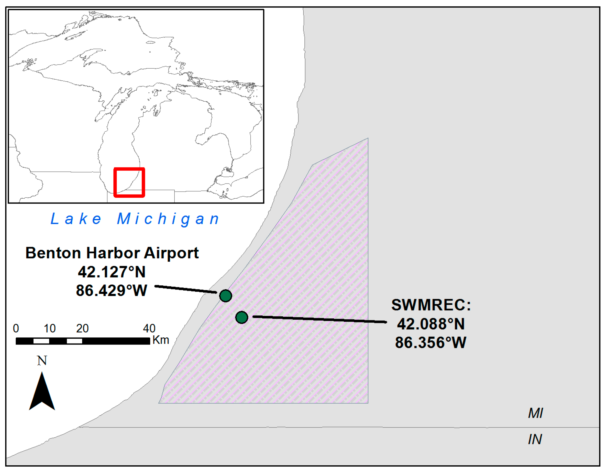
2.1. Study Area
2.2. Data
2.3. Methods
3. Results
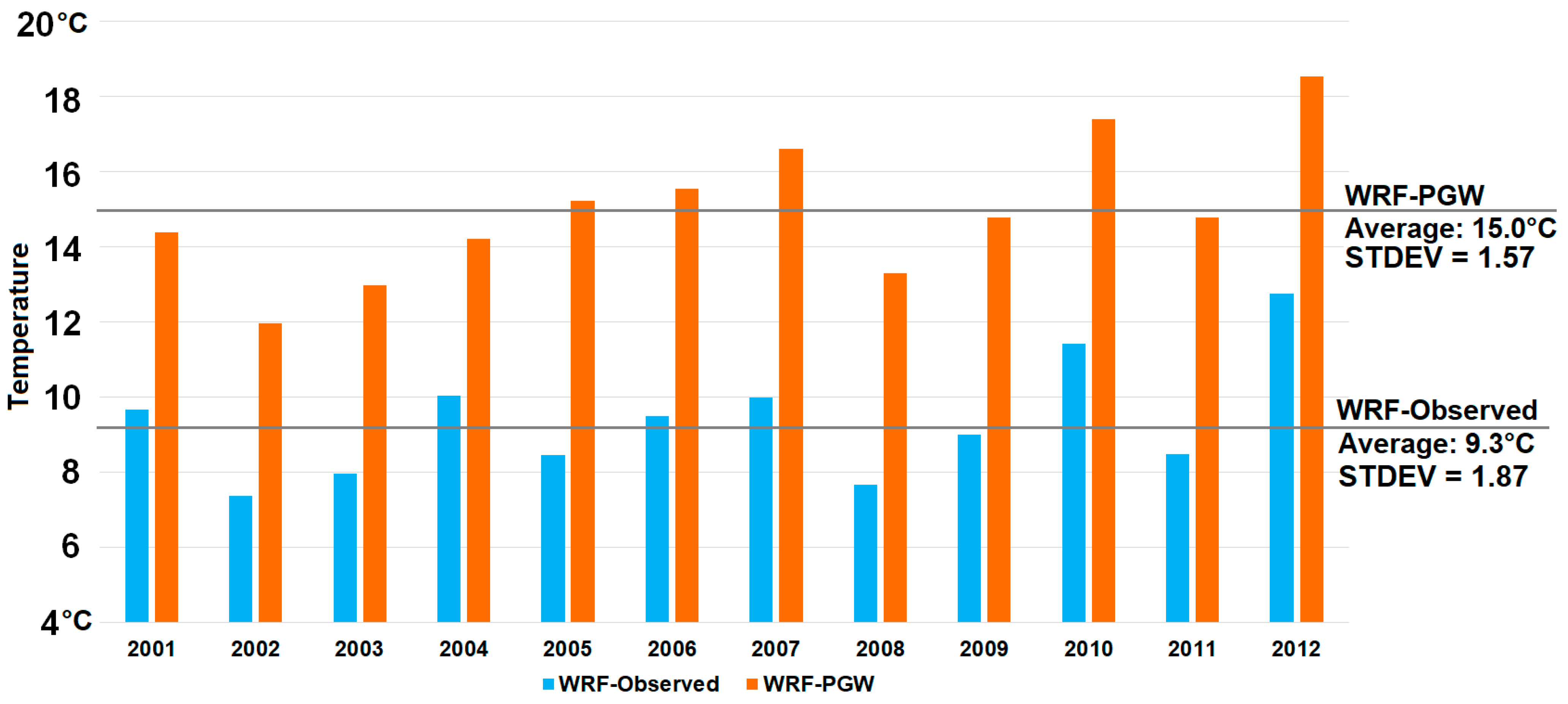
3.1. Effects on Spring Temperature
3.2. Effects on GDD Accumulation
3.3. Effects on Potential Frost
4. Discussion
4.1. Implications for Viticulture in Study Area
4.2. Implications for Global Viticulture
5. Conclusions
Author Contributions
Funding
Institutional Review Board Statement
Informed Consent Statement
Data Availability Statement
Conflicts of Interest
References
- Jones, G. Climate change and the global wine industry. In Proceedings of the 13th Annual Australian Wine Industry Technical Conference, Adelaide, Australia, 28 July–2 August 2007. [Google Scholar]
- Schultze, S.R.; Sabbatini, P.; Luo, L. Effects of a warming trend on cool climate viticulture in Michigan, USA. SpringerPlus 2016, 5, 1119. [Google Scholar] [CrossRef] [PubMed] [Green Version]
- Schultze, S.R.; Sabbatini, P.; Luo, L. Interannual effects of early season growing degree day accumulation and frost in the cool climate viticulture of Michigan. Ann. Assoc. Am. Geogr. 2016, 106, 975–989. [Google Scholar] [CrossRef]
- Zabadal, T.; Andresen, J.A. Vineyard establishment I: Site selection, vineyard design, obtaining grapevines, and site preparation. Mich. State Univ. Ext. Bull. 1997, E-2644, 23. [Google Scholar]
- Zabadal, T.; Dami, I.; Goffinet, M.; Martinson, T.; Chien, M. Winter injury to grapevines and methods of protection. Mich. State Univ. Ext. Bull. 2007, E2930, 105. [Google Scholar]
- Schultze, S.R.; Sabbatini, P.; Andresen, J.A. Spatial and temporal study of climatic variability on grape production in southwestern Michigan. Am. J. Enol. Vitic. 2014, 65, 179–188. [Google Scholar] [CrossRef]
- Bowman, S. Spring vine management: The pros and cons of frost fans vs sprinkler systems. Aust. N. Z. Grapegrow. Winemak. 2018, 656, 25. [Google Scholar]
- Wang, H.; Dami, I.E. Evaluation of budbreak-delaying products to avoid spring frost injury in grapevines. Am. J. Enol. Vitic. 2020, 71, 181–190. [Google Scholar] [CrossRef]
- Madelin, M.; Beltrando, G. Spatial interpolation-based mapping of the spring frost hazard in the Champagne vineyards. Meteorol. Appl. 2005, 12, 51–56. [Google Scholar] [CrossRef]
- Kartschall, T.; Wodinski, M.; von Bloh, W.; Oesterle, H.; Rachimow, C.; Hoppmann, D. Changes in phenology and frost risks of Vitis vinifera (cv Riesling). Meteorol. Z. 2015, 24, 189–200. [Google Scholar] [CrossRef]
- Shaw, A.B. The Niagara Peninsula viticultural area: A climatic analysis of Canada’s largest wine region. J. Wine Res. 2005, 16, 85–103. [Google Scholar] [CrossRef]
- Molitor, D.; Caffarra, A.; Sinigoj, P.; Pertot, I.; Hoffmann, L.; Junk, J. Late frost damage risk for viticulture under future climate conditions: A case study for the Luxembourgish winegrowing region. Aust. J. Grape Wine Res. 2014, 20, 160–168. [Google Scholar] [CrossRef]
- Meier, M.; Fuhrer, J.; Holzkämper, A. Changing risk of spring frost damage in grapevines due to climate change? A case study in the Swiss Rhone valley. Int. J. Biometeorol. 2018, 62, 991–1002. [Google Scholar] [CrossRef] [PubMed] [Green Version]
- Leolini, L.; Moriondo, M.; Fila, G.; Costafreda-Aumedes, S.; Ferrise, R.; Bindi, M. Late spring frost impacts on future grapevine distribution in Europe. Field Crop. Res. 2018, 222, 197–208. [Google Scholar] [CrossRef]
- Evans, K.J.; Bricher, P.K.; Foster, S.D. Impact of frost injury incidence at nodes of Pinot Noir on fruitfulness and growth-stage lag. Aust. J. Grape Wine Res. 2019, 25, 201–211. [Google Scholar] [CrossRef]
- Sommers, B.J. The Geography of Wine: How Landscapes, Cultures, Terroir, and the Weather Make a Good Drop; Penguin: London, UK; p. 304.
- de Blij, H.J. Geography of viticulture: Rationale and resource. J. Geogr. 1983, 82, 112–121. [Google Scholar] [CrossRef]
- Van Leeuwen, C.; Friant, P.; Chone, X.; Tregoat, O.; Koundouras, S.; Dubourdieu, D. Influence of climate, soil, and cultivar on terroir. Am. J. Enol. Vitic. 2004, 55, 207–217. [Google Scholar]
- Amerine, M.; Winkler, A. Composition and quality of musts and wines of California grapes. Hilgardia 1944, 15, 493–675. [Google Scholar] [CrossRef] [Green Version]
- Olmo, H.P. A Survey of the Grape Industry of Western Australia; Vine Fruits Research Trust: Perth, Australia, 1956. [Google Scholar]
- Huglin, P. Nouveau mode d’évaluation des possibilités héliothermiques d’un Milieu viticole. C. R. Seances Acad. Agric. Fr. 1978, 64, 1117–1126. [Google Scholar]
- Pfister, C. Variations in the Spring-Summer Climate of Central Europe from the High Middle Ages to 1850; Springer: Berlin/Heidelberg, Germany, 1988. [Google Scholar]
- Gladstones, J. Viticulture and Environment; Winetitles: Adelaide, Australia, 1992. [Google Scholar]
- Jones, G.V.; Davis, R.E. Climate influences on grapevine phenology, grape composition, and wine production and quality for Bordeaux, France. Am. J. Enol. Vitic. 2000, 51, 249–261. [Google Scholar]
- Cook, B.I.; Wolkovich, E.M. Climate change decouples drought from early wine grape harvests in France. Nat. Clim. Chang. 2016, 6, 715–719. [Google Scholar] [CrossRef]
- Bindi, M.; Miglietta, F.; Gozzini, B.; Orlandini, S.; Seghi, L. A simple model for simulation of growth and development in grapevine (Vitis vinifera L.). II. Model validation. VITIS 1997, 36, 73–76. [Google Scholar]
- Garcia de Cortazar, I.; Seguin, B. Climate warming: Consequences for viticulture and the notion of terroirs in Europe. In Proceedings of the VII International Symposium on Grapevine Physiology and Biotechnology, Davis, CA, USA, 21–25 June 2004; Volume 689, pp. 61–70. [Google Scholar]
- Jones, G.V.; White, M.A.; Cooper, O.R.; Storchmann, K. Climate change and global wine quality. Clim. Change 2005, 73, 319–343. [Google Scholar] [CrossRef]
- Schultz, H.R.; Jones, G.V. Climate induced historic and future changes in viticulture. J. Wine Res. 2010, 21, 137–145. [Google Scholar] [CrossRef]
- Blanco-Ward, D.; Monteiro, A.; Lopes, M.; Borrego, C.; Silveira, C.; Viceto, C.; Rocha, A.; Ribeiro, A.; Andrade, J.; Feliciano, M.; et al. Analysis of climate change indices in relation to wine production: A case study in the Douro region (Portugal). In Proceedings of the BIO Web of Conferences 2017, Sofia, Bulgaria, 29 May–2 June 2017; Volume 9, p. 1011. [Google Scholar]
- Moriondo, M.; Jones, G.V.; Bois, B.; Dibari, C.; Ferrise, R.; Trombi, G.; Bindi, M. Projected shifts of wine regions in response to climate change. Clim. Chang. 2013, 119, 825–839. [Google Scholar] [CrossRef]
- Santillán, D.; Iglesias, A.; La Jeunesse, I.; Garrote, L.; Sotes, V. Vineyards in transition: A global assessment of the adaptation needs of grape producing regions under climate change. Sci. Total Environ. 2019, 657, 839–852. [Google Scholar] [CrossRef] [PubMed]
- Nemoto, M.; Hirota, T.; Sato, T. Prediction of climatic suitability for wine grape production under the climatic change in Hokkaido. J. Agric. Meteorol. 2016, 72, 167–172. [Google Scholar] [CrossRef] [Green Version]
- Firth, R.; Kala, J.; Lyons, T.J.; Andrys, J. An analysis of regional climate simulations for Western Australia’s wine regions—model evaluation and future climate projections. J. Appl. Meteorol. Climatol. 2017, 56, 2113–2138. [Google Scholar] [CrossRef]
- Dunn, M.; Rounsevell, M.D.; Boberg, F.; Clarke, E.; Christensen, J.; Madsen, M.S. The future potential for wine production in Scotland under high-end climate change. Reg. Environ. Chang. 2019, 19, 723–732. [Google Scholar] [CrossRef] [Green Version]
- Koppen, W. Versuch einer klassifikation der klimate, vorzugsweise nach ihren beziehungen zur pflanzenwelt. Geogr. Z. 1900, 6, 593–611. [Google Scholar]
- Geiger, R. The Climate near the Ground; Harvard University Press: Cambridge, MA, USA, 1965. [Google Scholar]
- Andresen, J.A.; Winkler, J.A. Weather and climate. Chapter 19. In Michigan Geography and Geology; Schaetzl, R.J., Brandt, D., Darden, J.T., Eds.; Pearson Custom Publishing: Boston, MA, USA, 2009; pp. 288–314. [Google Scholar]
- Assel, R.A.; Quinn, F.H.; Leshkevich, G.A.; Bolsenga, S.J. Great Lakes Ice Atlas; National Oceanic and Atmospheric Administration, Environmental Research Laboratories, Great Lakes Environmental Research Laboratory: Ann Arbor, MI, USA, 1983. [Google Scholar]
- Assel, R.A.; Robertson, D.M. Changes in winter air temperatures near Lake Michigan, 1851–1993, as determined from regional lake-ice records. Limnol. Oceanogr. 1995, 40, 165–176. [Google Scholar] [CrossRef]
- Moroz, W.J. A lake breeze on the eastern shore of Lake Michigan: Observations and model. J. Atm. Sci. 1967, 24, 337. [Google Scholar] [CrossRef] [Green Version]
- USDA-NASS. Quick Stats, Berrien County (MI); USDA-NASS: Washington, DC, USA, 2016.
- Hathaway, L.; Kegerreis, S. The History of Michigan Wines: 150 Years of Winemaking Along the Great Lakes; The History Press: Cheltenham, UK, 2010. [Google Scholar]
- Vanderweide, J.; Sabbatini, P.; Howell, G.S. Back to the future. A historical viticulture perspective on the Michigan grape industry. Wine and Vines, June 2017; 61–64. [Google Scholar]
- Schultze, S.R. Effects of Climate Change and Climate Variability on the Michigan Grape Industry. Ph.D. Dissertation, Michigan State University, East Lansing, MI, USA, 2015. [Google Scholar]
- Schultze, S.R.; Sabbatini, P. Implications of a climate-changed atmosphere on cool-climate viticulture. J. Appl. Meteorol. Clim. 2019, 58, 1141–1153. [Google Scholar] [CrossRef]
- Rasmussen, R.; Liu, C. High Resolution WRF Simulations of the Current and Future Climate of North America. NCAR Research Data Archive, Computational and Information Systems Laboratory. 2017. Available online: https://rda.ucar.edu/datasets/ds612.0/ (accessed on 6 January 2018).
- Orlanski, I. A rational subdivision of scales for atmospheric processes. Bull. Am. Meteorol. Soc. 1975, 56, 527–530. [Google Scholar]
- Oke, T.R. Boundary Layer Climates; Routledge: Oxfordshire, UK, 1978. [Google Scholar]
- Riahi, K.; Grübler, A.; Nakicenovic, N. Scenarios of longterm socio-economic and environmental development under climate stabilization. Technol. Forecast. Soc. Chang. 2007, 74, 887–935. [Google Scholar] [CrossRef]
- Van Vuuren, D.; Edmonds, P.; Kainuma, J.; Riahi, K.; Thomson, A.; Hibbard, K.; Rose, S.K. The representative concentration pathways: An overview. Clima. Chang. 2011, 109, 5–31. [Google Scholar] [CrossRef]
- National Climate Data Center. Benton Harbor Airport Station USC00200710 1950 to 2000. 2020. Available online: https://gis.ncdc.noaa.gov/maps/ncei/cdo/daily (accessed on 24 March 2020).
- McMaster, G.S.; Wilhelm, W.W. Growing degree-days: One equation, two interpretations. Agric. For. Meteorol. 1997, 87, 291–300. [Google Scholar] [CrossRef] [Green Version]


| Year | March | April | May |
|---|---|---|---|
| 2001 | 4.76 | 4.51 | 4.82 |
| 2002 | 4.58 | 4.20 | 5.05 |
| 2003 | 5.39 | 5.07 | 4.57 |
| 2004 | 3.75 | 4.31 | 4.49 |
| 2005 | 7.99 | 4.64 | 7.66 |
| 2006 | 6.37 | 5.65 | 6.18 |
| 2007 | 6.73 | 7.05 | 6.04 |
| 2008 | 7.24 | 4.76 | 4.92 |
| 2009 | 6.03 | 6.57 | 4.70 |
| 2010 | 7.93 | 4.72 | 5.32 |
| 2011 | 5.79 | 5.71 | 7.42 |
| 2012 | 5.68 | 6.95 | 4.69 |
| Mean | 6.02 | 5.35 | 5.49 |
| Year | March | April | May | Total |
|---|---|---|---|---|
| 2001 | 3 | 101 | 147 | 251 |
| 2002 | 11 | 55 | 119 | 186 |
| 2003 | 46 | 84 | 139 | 269 |
| 2004 | 29 | 62 | 124 | 215 |
| 2005 | 53 | 103 | 219 | 375 |
| 2006 | 45 | 136 | 173 | 354 |
| 2007 | 81 | 126 | 185 | 392 |
| 2008 | 27 | 83 | 143 | 253 |
| 2009 | 35 | 113 | 140 | 288 |
| 2010 | 108 | 114 | 152 | 373 |
| 2011 | 22 | 102 | 219 | 342 |
| 2012 | 98 | 158 | 145 | 400 |
| Mean | 46 | 103 | 159 | 308 |
| Year | Less Days in PGW | Less Hours < −1 °C in PGW |
|---|---|---|
| 2001 | 22 | 284 |
| 2002 | 18 | 219 |
| 2003 | 12 | 212 |
| 2004 | 13 | 161 |
| 2005 | 14 | 237 |
| 2006 | 22 | 208 |
| 2007 | 19 | 287 |
| 2008 | 23 | 314 |
| 2009 | 17 | 173 |
| 2010 | 10 | 109 |
| 2011 | 18 | 202 |
| 2012 | 6 | 57 |
| 2013 | 30 | 380 |
| Total | 224 | 2843 |
Publisher’s Note: MDPI stays neutral with regard to jurisdictional claims in published maps and institutional affiliations. |
© 2022 by the authors. Licensee MDPI, Basel, Switzerland. This article is an open access article distributed under the terms and conditions of the Creative Commons Attribution (CC BY) license (https://creativecommons.org/licenses/by/4.0/).
Share and Cite
Schultze, S.R.; Sabbatini, P. Impact of Early Season Temperatures in a Climate-Changed Atmosphere for Michigan: A Cool-Climate Viticultural Region. Atmosphere 2022, 13, 251. https://doi.org/10.3390/atmos13020251
Schultze SR, Sabbatini P. Impact of Early Season Temperatures in a Climate-Changed Atmosphere for Michigan: A Cool-Climate Viticultural Region. Atmosphere. 2022; 13(2):251. https://doi.org/10.3390/atmos13020251
Chicago/Turabian StyleSchultze, Steven R., and Paolo Sabbatini. 2022. "Impact of Early Season Temperatures in a Climate-Changed Atmosphere for Michigan: A Cool-Climate Viticultural Region" Atmosphere 13, no. 2: 251. https://doi.org/10.3390/atmos13020251