Hydroclimatology of the Chitral River in the Indus Basin under Changing Climate

Abstract

Biased distribution of hydro-climate stations in high elevations are major obstacles for reliable appraisal of the hydro-climatic regime of the Chitral Basin located in the extreme north of Pakistan. We modeled this regime in the ARC-SWAT hydrological model forced with the latest gridded reanalysis ERA5 Land dataset, bias-corrected against a good quality reference dataset. The performance of the gridded dataset was cross-validated by comparing the model flow simulation against the observed flows. The ERA5 Land overall provided reasonably good estimates. The calibrated model on the daily time scale was able to provide excellent values of the employed statistical measures (NSE, KGE, PBIAS, RMSE and MAE). For a future climate change analysis, climate series was devised using two future projection scenarios (RCP4.5 and RCP8.5) using the best performing GCM (MIROC5_rlilp1) out of five investigated GCMs. The results of the climate change analysis reveal increment in the average temperature up to +3.73 °C and +5.62 °C for RCP4.5 and RCP8.5, respectively, while the analysis of precipitation suggests an annual decrease up to −16% and −35% against RCP4.5 and RCP8.5, respectively, by the end of century. A future simulated flow analysis showed an increment of +0.25 % and decrease of −6.82% for RCP4.5 and RCP8.5, respectively. Further analysis of climate suggests seasonal deflections especially in precipitation and flow regimes. A notable climb in flow quantities was observed during spring season (MAM) in spite of the major reduction in precipitation amounts for that season. This implicitly supports a high rate of glacial/snow melt especially in the spring season during that period. Frequent droughts and floods are also projected by examining flow durations at each interval of the 21st century.

1. Introduction

Climate change is recognized to accelerate and intensify the potential water resources related to cataclysm events at various scales. The zenith of the industrial era during the 2nd half of the 20th century instigated high emissions of anthropogenic greenhouse gases into the atmosphere leading to a significant alteration in global climate. The threat of the changing climate is continuously rising due to uninterrupted emission of greenhouse gases [1]. The impacts of rising temperatures have the potential to cause changes in frequency, variation, and magnitude of other atmospheric variables such as precipitation [2,3,4]. Precipitation along with temperature has close ties with the catchment scale hydrological features. Therefore, the climate change anomaly can significantly impact the runoff and other climate sensitive parameters of the basin [5,6]. Accurate observation and proper examination of these variables can help to derive appropriate strategies for managing water resources on a regional or basin scale. However, despite many advances, reliable climate projections, especially in higher mountainous terrains, are difficult to achieve due to the lack of observations and directional biases of the available observations [7].

Chitral River is the largest tributary of the Kabul River which ultimately feeds to the Indus River near Attock. The Chitral River derives its major share of water from melting snow and glaciers in the Hindukush Mountain range for which winter precipitation serves as the primary source of replenishment. Despite a multitude of studies on the Upper Indus Basin, the reliability of precipitation at sub-basin scale still remains difficult and non-intuitive [7,8,9]. There are only a few hydroclimatological studies focusing the Chitral Basin alone, most of the previous studies have aimed Indus and Kabul Basins as a whole. These studies suggest the consistent rise of river flows with respect to the increase in temperature. However, uncertainty persists in precipitation estimates. For instance, some studies have predicted a reduction in mean annual precipitation in the Chitral Basin [10,11], while others have reported a substantial increase, predominantly during the winter season [3,12,13]. Additionally, the reported increase in snow cover of the Chitral Basin area implicitly suggests a precipitation increase during the winter season [14]. Reliable estimation of the future climate requires accurate observations and evaluation of contemporary variables; therefore, the quest for accuracy continues.

Almost, 21% of the Chitral territory on the Pakistani side consists of perennial snow or glaciers with highly steep ravines, which make it difficult to install and operate climatic stations [14]. The basin has the station density of only one station to cover 7300 sq. km of area, which is well-below the standards suggested by the World Meteorological Organization (WMO) (limit of one per 250 sq.km for mountainous terrain). Therefore, the observational network inadequately depicts the high-altitude precipitation variations [7,9]. For countering the spatial heterogeneity, various studies utilized the gridded datasets mostly based on three types; station-based, satellite-based, and reanalysis (atmospheric model-based) [15,16]. Station-based precipitation datasets utilize conventional station climate data. In the northern side, stations are mostly installed at lower and drier valleys corresponding to higher altitude locations which seem to suggest an underestimated spatial interpolation [16]. In addition to this, existence of a systematic bias is another reason for the underestimation of precipitation [7].

Use of satellite-gridded data is another alternative option that has extensively been used for climate change projections and hydrological analysis [17]. These products make use of infrared (IR) observations of cloud cover and passive microwave (PW) for precipitation measurements. In spite of improved performance over the flat terrains, it is reported to face difficulty estimating precipitation across the higher altitude complex terrains where precipitation is significantly influenced by orography [17,18]. Satellite data often require land observations for their ground truthing and calibration which indicates their dependency on the quality of observed data [16].

Reanalysis products offer useful alternatives to avail precipitation and other climatic variables as predicted outputs of model assimilation. These models are typically called Numerical Weather Predictors (NWPs). This computation uses numerical algorithms bounded by the physical laws which allow to forecast a wide range of variables. These variables are the result of numerical modeling; hence, they are not influenced by the direct observations especially for precipitation and become susceptible to uncertainty and model biases. Various studies have highlighted different aspects of reanalysis products [16,19,20]. Nevertheless, continuous developments are being made to overcome their deficiencies related to improved computations, data assimilations and advanced retrieval of ground and atmosphere data from satellites [21,22,23].

During physical-based modeling, uncertain observational data reduce the value of the model. A calibrated model often produces good results but at the same time undermines the actual physical response of the catchment. Therefore, incorporating accurate precipitation data is a crucial step for developing a reliable parameterized model [24]. In order to overcome the observational deficiencies, the hydrometeorologists generally use gridded datasets. However, their accuracy is very much dependent on the quality of their input data and robustness of the computational methods. Dahri et al. [25] evaluated precipitation estimates of 27 widely used gridded datasets for the high-altitude Upper Indus Basin using [7] dataset as the reference and determined the 5th generation European Centre for Medium-Range Weather Forecasts ECMWF Re-Analysis (ERA5) dataset to be relatively more accurate than the other products. ERA5 was also attested in the region by [16], who cross-validated 20 gridded datasets including ERA5 over the Indus Basin and highlighted better performance by the ERA5. ERA5 Land is a reiteration of the land component of ERA5 for a land-based analysis at a finer resolution of 9 km by applying the lapse rate correction to account for the influence of the altitude on the spatial structure of the weather variables [21].

Attaining reliable observations over the Upper Indus Basin can be a difficult task [9]. Gauge precipitation is generally exposed to systematic biases. The usual causes behind these systematic biases are topography, gauge types, surrounding vegetation, wind, and temperature. These biases are detrimental for the reliabilities of observed data especially at higher altitudes where wind induced systematic biases are dominant. The wind induced errors persist as a large source of uncertainty and major responsibility for the under estimation of solid precipitation which is a core format of precipitation during winter. For the adjustment of these biases WMO set standard procedures for the correction; however, most of the global precipitation products neglected such standards which can exacerbate the reliability of those datasets [7]. Dahri et al. [7] adjusted these systematic biases by precipitation measuring stations over the Upper Indus Basin. Therefore, their dataset can serve as a reference dataset for this research study.

Climate forecasts require development and use of accurate climate models. Regional Climate Models (RCMs) are widely used for regional climate analysis and are constantly being improved. However, some internal and external uncertainty associated with systematic biases, sensitivity to numerical schemes, and resolution-depended processes still persist [10]. Therefore, downscaled and bias-corrected GCMs are often preferred to provide a more accurate depiction at a regional scale [26]. Recently, [25] evaluated 75 GCM outputs to single out the most suitable model based on their past performance for the high-altitude Indus Basin. From the overall analysis 2 GCMs (MIROC5_rlilp1 and MPI_ESM_LR_rlilpl) were selected to represent two extremes of wet-warm and dry-cold scenarios.

The lack of climate data can partly be compensated by hydrological modeling, but uncertainties in observational data reduce value of hydrological modeling [27]. Generally, a calibrated model often produces good results but at the same time, undermines the actual physical response of catchment. Therefore, accuracy and reliability of precipitation data is a crucial step for pragmatic hydrological modeling.

Our research is intended to appraise the hydroclimatological implications over the high-altitude Chitral Basin with the aid of an ERA5 Land reanalysis. This study will provide better insights and projections of hydro-climate parameters essential for hydropower and water balance studies.

2. Materials and Methods

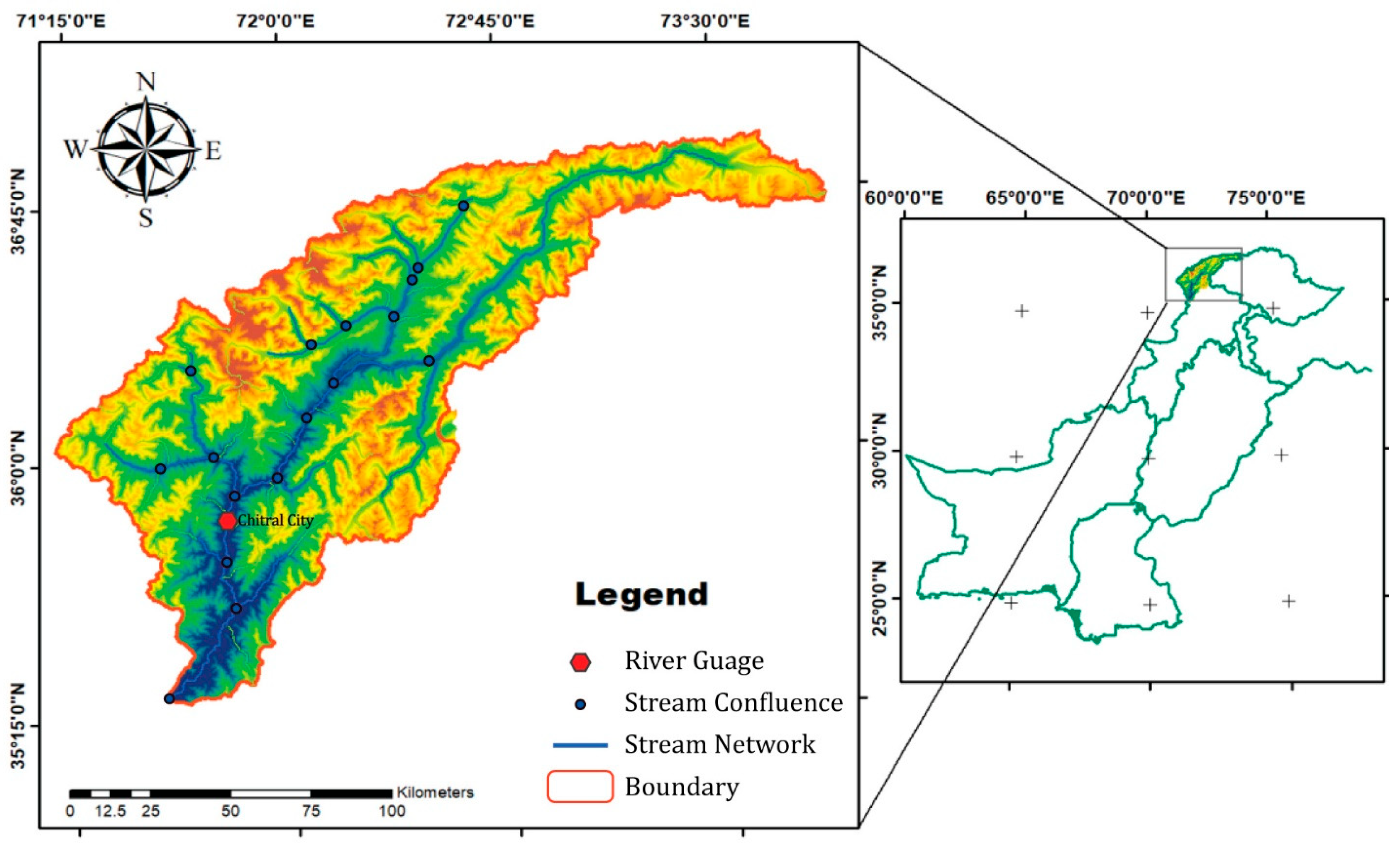
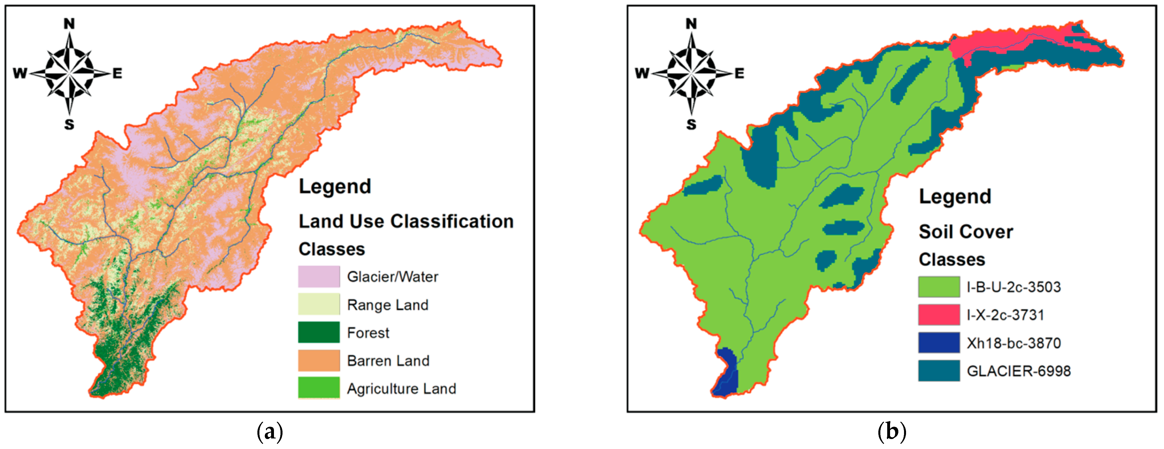
2.1. Study Area

The Chitral Basin is a transboundary basin between Afghanistan and Pakistan. However, this study covers the area located in the north-west of Pakistan, administered under the district Chitral of Khyber Pakhtunkhwa province (Figure 1). It is located between 35°–37° N latitudes and 70°–74° E longitudes with the drainage area of 14639.54 km². Almost 50% of total area has a land slope of more than 65% and only 2.6% has a relatively flat terrain slope (0–12%). The upper part consists of high mountainous terrain of the Hindukush Mountain ranges and attains 7700 m height, while lower valleys at the southern part stand around 1100 m above mean sea level. The mean elevation of the Chitral Basin lies at 4180 m above sea level.

The climate of Chitral valley is considered cold and dry. Summer monsoon rainfall has little influence over the Chitral Basin, while the majority of rainfall occurs during winter and spring mostly as snow, which is sourced from the westerly winter disturbance of Mediterranean. The average annual precipitation observed over the period of (1992–2017) at Chitral is 465 mm.

Approximately 14.5% of the basin area occupies snow/glacier cover, which is the key source of water supply to the Chitral River and its tributaries. The Chitral River originates from the northern mountain ranges of Hindukush as the Mastuj river. Seasonal snow melt is a major contributor of discharge throughout the year. About 73% of the total precipitation in the basin is received during the October–April months and the majority of it falls in the form of snow. Peak flows occur during the monsoon season in June to September. The average flow rate of the Chitral River recorded at the Chitral city gauge is 292 cumec between the periods of 2003 to 2015. Other major tributaries that contribute to the Chitral River are Yarkhon River, Turkho River, Ludkho River, Turich River, and Golen Gol River.

Chitral River has the considerable potential to contribute to the economies of both Pakistan and Afghanistan via power and irrigation sectors. Therefore, it is imperative to investigate the current and future climate changes and the associated hydrological implications.

2.2. Datasets

2.2.1. Climate Datasets

Adjudicating the hydrological response of any catchment often becomes difficult if the area is deficient in hydrometeorological observations. The Chitral Basin is difficult to access due to rugged and high-mountain terrain, making installation and operation of climate stations troublesome. The existing meteorological stations are highly biased towards low altitude valleys [7,9,28]. Moreover, the presence of systematic measurement errors can seriously aggravate the quality of observations and associated hydroclimatological analyses. Therefore, gridded datasets are important means to compensate the spatio-temporal limitations of the point observations. A study conducted by [7] reported to recover a significant portion of precipitation over high altitudes of the Indus Basin which was previously undermined by the climatic stations, due to measurement errors. This study takes monthly climatologies (1999–2011) determined by [7] as references to bias correct the temperature (minimum and maximum) and precipitation of gridded datasets. Recently, gridded precipitation datasets of the European Center for Medium-Range Weather Forecast (ECMWF) were able to provide better estimates of climate parameters, especially precipitation, over the Indus Basin compared with other gridded datasets [16,28]. The latest addition to the ECMWF family is ERA5 Land, which is specifically derived from the rerun of land component of ERA5. Considerable improvements are implemented such as refinement of the resolution grid up to 1 h time step and 9 km square grid. This allows increased accuracy to fill for a wide range of land-based applications. In addition to that, ERA5 Land is computationally efficient as no data assimilation takes places. Improvements are also made to counter the influence of altitude by applying a lapse rate correction to climate parameters [29,30]. The dataset was acquired from Copernicus Climate Change Service [31].

2.2.2. Future Climate Projection

Climate change projections are generally derived by mathematical models known as a General Circulation Model (GCM). Their projections of the future climate are dependent upon global socio-economic-based scenarios and are expressed in terms of Representative Concentration Pathways (RCPs). Among the four of RCPs, we considered using the most near to usual scenario and worst-case scenario based upon the assumption that carbon emissions are still increasing dangerously and will continue to grow more; therefore, the most optimistic scenario such as RCP2.6 is seemingly difficult to happen in the future. The scenarios most resembling these conditions are RCP4.5 (moderate stabilization scenario) and RCP8.5 (extreme emission scenarios). Currently, a wide number of GCMs are used for simulating climate; however, a similarly higher number of output variability also persists, which makes the analysis vague for judging future climate responses [27]. Amidst these circumstances, we emphasize choosing from a few numbers of GCMs for catering uncertainty. The criteria of initial selection are defined by the performance shown by GCMs previously over the region.

Recently, [25] examined various GCMs for the high-altitude Indus Basin and filtered out the high-performing GCMs. MIROC5 and MPI-ESM-LR were found to be at better attaining higher scores to reproduce the historical climate. Similarly, [27] also appraised the performance of several GCMs including MIROC5, over the same region. We evaluated a few of those best performing GCMs for our analysis. The selected GCMs included MIROC5_r1i1p1, MIROC5_r2i1p1, CMCC-CMS_r1i1p1, MPI-ESM-LR_r1i1p1, and MPI-ESM-LR_r3i1p1, and then selected the best suited GCM for the selected study region for a future hydro-climatic analysis. The details of five GCMs are provided in Table S1.

2.3. Methodolgy

2.3.1. Bias Correction

The accuracy of reanalysis products is limited by their inherited model biases when compared with the observed climate data. Therefore, they often require bias correction prior to carrying out the analysis of variables [21]. Many studies [32,33,34] have carried out the performance evaluation of the bias correction techniques and mostly suggest the dependency on the location. Shrestha et al. [32] carried out the comparison between the simpler linear bias correction and intricate quantile delta mapping technique upon the Himalayan terrain pre-dominated by high altitude orography. Their findings suggest that the intricate techniques can be avoided for monthly analysis without compromising reliability. Climate in the Chitral River Basin is mainly governed by the high-altitude orography [32] and our requirement to analyze the future climate change is limited to a monthly scale; therefore, we used the simpler linear bias correction technique for correction in climate data. ERA5 Land reanalysis was bias-corrected using the monthly climatology (1999–2011) of [7] for the period of 1981 to 2015.

The equations are provided below:

$$\mathrm{Phis}(d)*=\mathrm{Phis} (d).\frac{Um.\left\{Pobs\left(d\right)\right\}}{Um\{Phis \left(d\right)\}}$$

(1)

$$\mathrm{Psim}(d)*=\mathrm{Psim} (d).\frac{Um.\left\{Pobs\left(d\right)\right\}}{Um\{Phis \left(d\right)\}}$$

(2)

$$\mathrm{This}(d)*=\mathrm{This} (d).[ Um.\left\{Tobs\left(d\right)\right\}-Um.\left\{This\left(d\right)\right\}]$$

(3)

$$\mathrm{Tsim}(d)*=\mathrm{Tsim} (d).[ Um.\left\{Tobs\left(d\right)\right\}-Um.\left\{This\left(d\right)\right\}]$$

(4)

where P = precipitation, T = temperature, d means daily, Um = long term mean, * indicates bias-corrected, his refers to historical raw GCM data, obs stands for observed data and sim is the raw GCM future data.

2.3.2. SWAT Hydrological Model

Soil and Water Assessment Tool (SWAT) is a physically-based, semi distributed continuous-time model developed by the United States Development of Agriculture (USDA) to simulate multiple types of hydrological applications over a watershed scale on annual, monthly, and daily time steps [35]. It has been successfully executed and tested on various localities including snow and high-altitude topography [36,37]. It has also been used for various applications such as climate change analysis, land use, and management practices. SWAT allows ease and flexibility in data requirement [32,38]. The Hydrological process is carried out at Hydrological Response Units (HRUs) scale based on the water balance equation. The major hydrological processes considered in water balance are runoff, infiltration, evapotranspiration, lateral flows, and percolation.

Additionally, SWAT also allows the simulation of the snow conditions when the daily air temperature (SFTMP) becomes less than the provided threshold values of temperature, and then precipitation falling into that (HRU) is treated as snow. The liquid water equivalent of snowfall is incremented into snowpack. The volume of snowpack expands with auxiliary snowfall during the winter season and reduces during the subsequent summer season due to snow melt. The melting process is primarily controlled by snow melt temperature (SMTMP) in SWAT. SWAT equations are more broadly explained in [39].

Initially, SWAT required various input layers to generate watershed environment of corresponding actual basin. These input layers consist of a Digital Elevation Model (DEM), land use, and soil layer. The DEM of ASTER 30 m resolution was obtained from the USGS Earth explorer web plate form and the required tiles of DEM were mosaicked. The quality of the DEM is defined by its resolution and quality of its retrieval; finer resolution tends to well-define the elevation distribution across the topography. DEM in SWAT is essential for the delineation and projecting slopes of watershed. Land use classification is performed by defining the features of Landsat-7 30 m resolution satellite imagery via supervised classification. All the major land uses are fractioned into five categories; barren, rangeland, forest, agriculture, and water (glaciers and snow). For SWAT modeling, soil data of 1 km resolution was obtained from an open-sourced FAO [40]. The summary of the dataset and delineation are depicted in Figure 2.

Furthermore, to achieve more accuracy, the climate datasets were extracted for each of the model grids uniformly distributed across the watershed. After bias correction, the climate station files were input into two separate models distinguished by the RCP4.5 and RCP8.5 for better convenience. The model domain was divided into 10 elevation bands to obtain optimum variation.

2.3.3. Pre-Modeling Setup

Authenticity of model simulation is primarily adjudicated by the statistical performance of the model. The model is calibrated and validated using SWAT Calibration and Uncertainty Program (SWAT-CUP). SWAT-CUP permits the user to choose from multiple calibration algorithms for better performance. The Sequential Uncertainty Fitting (SUFI-2) algorithm which evaluates uncertainty between observed and simulated values, was selected because of its recognition to perform better in limited number of simulations [41,42]. The sensitive parameters related to flows were evaluated in same interface before model calibration. SUFI-2 offers two types of sensitivity analysis i.e., global and one-factor-at-a-time (OAT). This study utilizes OAT analysis due to its computational efficiency. In OAT all the other parameters are held constant and one parameter is allowed to change, its effects are then appraised on the model output. Three to five model runs are sufficient to obtain the model sensitivity. More details about the methods are explained in [43]. In our study 20 parameters were selected for sensitivity analysis. Among these, the first 14 parameters (listed in

Table 1. Selected sensitive parameter and their calibrated values in the Chitral River Basin.

Parameters	Description
Hydrological Parameters
r__CN2.mgt	SCS runoff curve number	0.00034
v__ALPHA_BF.gw	Base flow alpha factor (days)	0.99
v__GW_DELAY.gw	Groundwater delay (days)	85
v__GWQMN.gw	Threshold in the shallow aquifer for return flow to occur (mm)	89
v__GW_REVAP.gw	Groundwater ‘‘revap” coefficient	0.03
v__SLSUBBSN.hru	Average slope length (m)	55
v__HRU_SLP.hru	Average slope steepness (m/m)	0.03
v__OV_N.hru	Manning’s “n” value for overland flow	18
Snow and Elevation Band Parameters
v__SFTMP.bsn	Snowfall temperature (°C)	2.59
v__SMTMP.bsn	Snow melt base temperature (°C)	−1.90
v__SMFMX.bsn	Maximum snow melt rate during year of summer solstice (mm/°C-day)	2.00
v__TIMP.bsn	Snowpack temperature lag factor	0.44
v__TLAPS.sub	Temperature lapse rate (°C/Km)	−5.70
v__PLAPS.sub	Precipitation lapse rate (mm/Km)	301.25

) were selected for further calibration. The study follows a guideline explained in [44]. The calibration of the snow parameters were dealt separately and subset with elevation band parameters. The rest of the parameters were calibrated in a separated group. Therefore, two sets of parameters were selected for independent calibration. This configuration avoided identification issues as explained in [44] in the parameterization section. To check the robustness of the model, the study follows a method used by [25], in which two validation periods were considered, one before the calibration period (backward validation) and the other after calibration (forward validation). This will provide the balanced overview of model performance for a longer time period.

For statistical evaluation of the model, five (5) objective functions were chosen based on past studies. For instance, [3] chose traditional metrics of Nash Sutcliff Efficiency (NSE) and Root Mean Square Error (RMSE) for evaluation of the UBC model over Kabul basin, [18] used Root Mean Square Error (RMSE) and Mean Absolute Error (MAE), while [25] recently used Modified Kling-Gupta Efficiency (KGE) and Percent Bias (PBIAS) for evaluation of the model performance. Furthermore, sensitivity of above-mentioned metrics are interlinked to each other and can be reformulated in relation to one another. For instance, the value of NSE is dependent upon the square of ratio between RMSE and the standard deviation ($S_{obs})$ of the observed value (see Equation (5)). Although, RMSE ranges from 0 to$\infty$, and close to 0 is desirable, it is also important to make sure it should be above a certain threshold to secure appropriate results. For examples, if RMSE =$S_{obs}$ then NSE = 0, similarly if RMSE is half the $S_{obs}$ then the value of NSE = 0.75. Further detail is provided in [45]. Therefore, we considered (NSE, KGE, PBIAS, RMSE and MAE) for evaluating the model performance. Equations of each objective function along with its range of values is provided below:

$$\mathrm{NSE}=1-\left[\frac{{{\displaystyle \sum }}_i^N{\left(Q_{obs,i}-Q_{sim,i}\right)}^2}{{{\displaystyle \sum }}_i^N{\left(Q_{obs,i}-Q^{*}{}_{obs}\right)}^2}\right],1-{\left[\frac{RMSE}{S_{obs}}\right]}^2 , (-\infty < \mathrm{NSE} < 1)$$

(5)

$$\begin{array}{c}\mathrm{KGE}=1-\sqrt{{\left(R-1\right)}^2+{\left(\beta -1\right)}^2+{\left(\gamma -1\right)}^2}, \beta =\frac{Q^{*}{}_{sim}}{Q^{*}{}_{obs}} , \gamma =\frac{S_{sim}/Q^{*}{}_{sim}}{S_{obs}/Q^{*}{}_{obs}}\\ (-\infty < \mathrm{KGE} < 1)\end{array}$$

(6)

$$\mathrm{PBIAS}=1-\left[\frac{{{\displaystyle \sum }}_i^N\left(Q_{obs,i}-Q_{sim,i}\right)}{{{\displaystyle \sum }}_i^N\left(Q_{obs,i}\right)}\right]\times 100 , (-\infty < \mathrm{PBIAS} < 100)$$

(7)

$$\mathrm{RMSE}=\sqrt{\frac{1}{N}{{\displaystyle \sum }}_i^N{\left(Q_{obs,i}-Q_{sim,i}\right)}^2}, (0 < \mathrm{RMSE} < \infty )$$

(8)

$$\mathrm{MAE}=\frac{{{\displaystyle \sum }}_i^N\left|\left(Q_{obs,i}-Q_{sim,i}\right)\right|}{N}, (0 < \mathrm{MAE} < \infty )$$

(9)

where N is the number of flow values, R is Pearson coefficient, Q_obs and Q_sim are the observed and simulated flows for ith observations, and Q*_obs and Q*_sim are the means of the observed and simulated flow values. S_obs and S_sim are the standard deviation of the corresponding observed and simulated flows. NSE indicates how closely the observed and simulated values fit the 1:1 line. NSE = 1 corresponds to a perfect match, 0 < NSE < 1 infers acceptable performance, NSE = 0 indicates that the model predictions are as accurate as the mean of the observed data, whereas NSE < 0 indicates that the observed mean is a better predictor than the simulated value inferring unacceptable performance. KGE values may range from −1 to +1 but its optimum value is 1. Any value of KGE provides the lower limit of its three components (Pearson’s correlation coefficient, bias, and variability ratio), meaning that the worst component is ≥to that value. The values of the other three indices are desired to be closer to zero.

3. Results and Discussion

3.1. Calibration and Validation Results

Due to the interlinking of precipitation and runoff, sparse precipitation observations along with the intricate orography of a region can negatively impact flow simulations [7,32,38]. Therefore, suitable calibration is essential to define the true relationship between these two imperative basin parameters. In our study we compared the model simulation to a single gauging station at Chitral city over Chitral River. The period of calibration was set to 10 years from (1996–2005), while a backward validation period of (1981–1995) and forward validation the period of (2006–2015) were selected.

Simulation of ERA5 Land model for the calibration period depicted in Figure 3 (daily basis) and Figure S1 (monthly basis) show a close resemblance to the observations. The model was able to precisely capture the synoptic trends of observational flow. Despite better representation, some discrepancies also need to be highlighted. For instance, the model was unable to accurately depict the flow recession toward the end of the years by over-estimating, furthermore exaggeration of peak flows were also simulated in multiple years.

The hydrological response of discharge was statistically evaluated on both daily and monthly scales (

Table 2. Statistical performance of SWAT model during calibration and validation periods.

Statistical Indicator	Backward-Validation (1981–1995)	Calibration (1996–2005)	Forward-Validation (2006–2015)
Daily Basis
NSE	0.79	0.84	0.78
KGE	0.82	0.91	0.85
PBIAS (%)	−15.65	1.15	−11.79
RMSE	136.61	117.87	129.91
MAE	88.51	78.10	85.89
Monthly Basis
NSE	0.87	0.90	0.86
KGE	0.82	0.92	0.85
PBIAS (%)	−15.66	1.15	−11.73
RMSE	99.87	85.80	96.20
MAE	68.46	58.34	62.61

). The mean and standard deviation of the observed and simulated values remain within appropriate range during the entire simulation period as indicated by NSE and KGE values. Similarly, values of PBIAS and MAE summarize the acceptable difference between ordinates of observed and simulated values. On average, RMSE remains less than half the standard deviation of observed values, which shows good model engagement. The values of the employed statistical measures indicate that the SWAT hydrological model was able to reproduce the river inflows quite well for the calibration as well as validation periods at both daily and monthly time scales. The observed and simulated river flows reveal excellent agreement. The model analysis also highlighted the significance of the reconciliation of the dataset from systematic biases as a reference dataset [7] was able to better adjust.

3.2. GCM Selection

Physically-based climate models are one of the key tools for quantifying the future hydro-climatic regime. Yet, despite substantial developments and increase in number of outputs, an understanding of the future climate remains vague and uncertain. Additionally, due to the inherited biases, multiple GCMs can produce different results leading to a misinterpretation of their outputs. Such problems are commonly encountered while using an ensemble, where a higher number of biased models can induce proclivity to results. Therefore, before quantifying the future regime, it is important to identify existent internal biases in GCM outputs first. As previously mentioned, for our concerning region we initially selected five GCMs based on the outcomes and observations of the previous studies, we then intended to evaluate internal seasonal bias for each product by comparing them with observation data.

The precipitation of five GCMs were differentiated into four periods, annual, winter (Oct–March), pre-monsoon (April-June) monsoon (July–Sep) and then evaluated by using the eight indices outlined in Table S2. At the end, GCMs were ranked according to their performance. MIROC5_r1i1p1 was found to achieve a high rank followed by MIROC5_r2i1p1. MIROC5_r1i1p1 showed the best performance for all four periods during analysis of the mean and attained rank 1 in the 5-day maximum rainfall, maximum dry spells length and maximum wet spells length on annual period. Conversely, the analysis also highlights considerable deficiencies, especially capturing dry and wet day lengths during the monsoon period. On the other hand, remaining GCMs were unable to provide consistency and shown substantial biases.

Similarly, four statistical indices (Mean Error, Standard Deviation Error, Root Mean Square Error, and Correlation Coefficient) outlined in Table S3 were selected for GCMs evaluation based on temperature. The result depicted MIROC5_r1i1p1 performance to be more robust. MIROC5_r1i1p1 outputs gained a superior score in three out of four indices. The final rankings of the five GCMs evaluated in this study are summarized in

Table 3. Final rankings of five GCMs evaluated.

GCM	Final Rankings
	Precipitation	Temperature
MIROC5_r1i1p1	1	1
MIROC5_r2i1p1	2	3
CMCC-CMS_r1i1p1	3	4
MPI-ESM-LR_r1i1p1	4	2
MPI-ESM-LR_r3i1p1	5	5

, while more details are provided in Tables S2 and S3. The independent analysis conducted in this study is in line with an earlier study for the high-altitude Upper Indus Basin [25]. Therefore, for future analyses, we selected MIROC5_r1i1p1 for deriving future hydro-climatic projections.

3.3. Hydroclimatological Projections

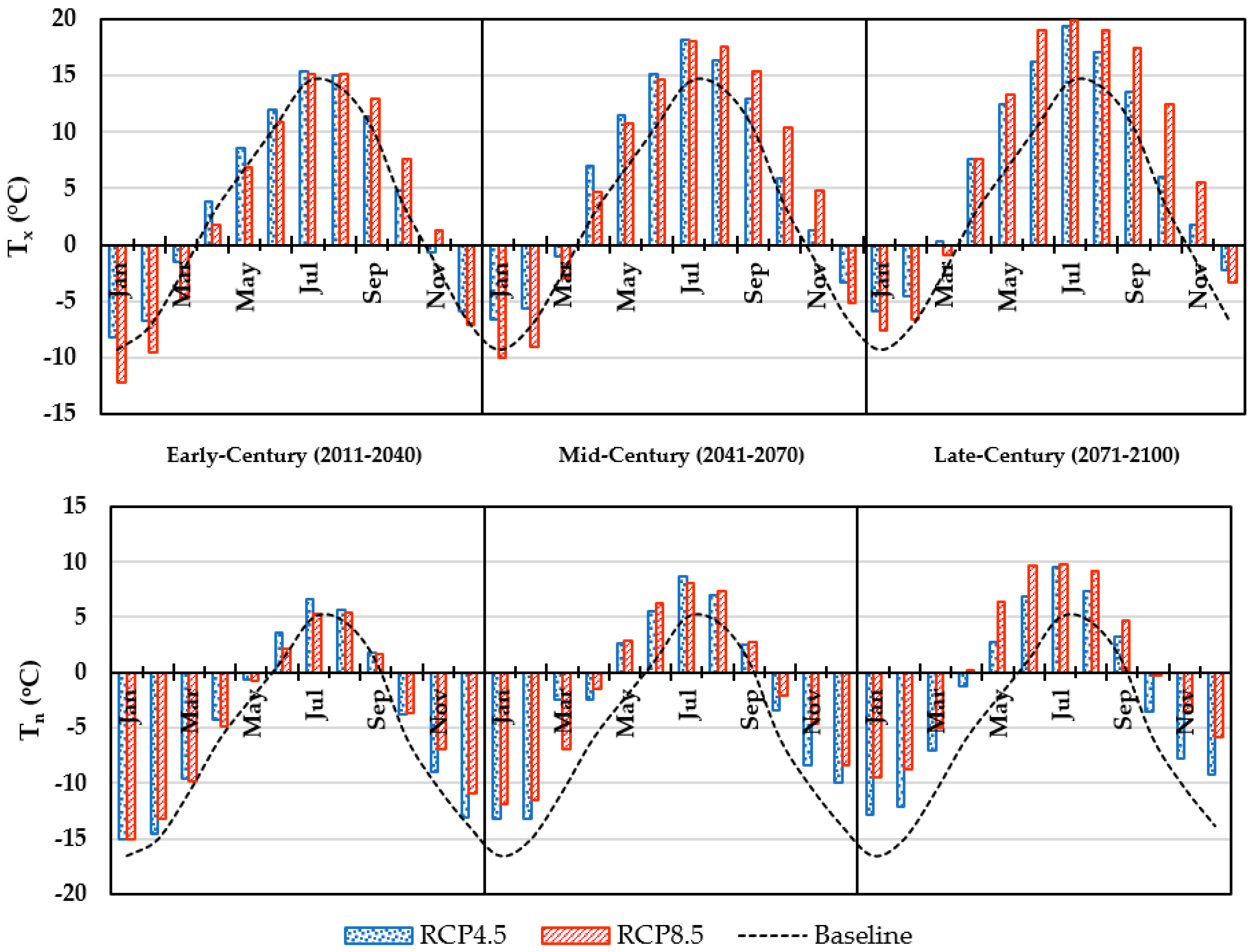
This research study quantified the climatic and hydrological projections for the three intervals of 21st century (early century 2011–2040, midcentury 2041–2070, and late century 2071–2100) with respect to median values during the baseline period of 1981–2010 under two climate scenarios of RCP4.5 and RCP8.5.

3.3.1. Temperature

Temperature is considered one of the sensitive indicators of climate change, which has a high tendency to cause instability in basin hydrology. Especially for the Chitral Basin, in which its glaciology is an important part of its hydrological implications, hence the study of temperature rise is highly intrinsic to determine its impact on the basin’s hydrology. Figure S2 displays the mean annual maximum and minimum temperature (T_x and T_n) for the historical and projected period. Additionally, the annual rate of rise was evaluated for the periods of baseline, early, mid and late century by mean of Sen‘s slope the Mann–Kendall trend analysis for providing more in-depth understanding of rate temperature rise shown in

Table 4. Projected temperature trends (°C) for RCP4.5 and RCP8.5 during early, mid, and late century.

Period	Tx (°C/Year)	Tn (°C/Year)	Tx (°C/Year)	Tn (°C/Year)
Baseline	0.018	0.014	0.018	0.014
	RCP4.5		RCP8.5
Early Century	0.082	0.079	0.072	0.097
Midcentury	0.053	0.042	0.081	0.074
Late Century	−0.032	−0.002	0.097	0.090

. Rate of rise recorded for the baseline period for T_x and T_n were 0.018 °C/year and 0.014 °C/year, respectively. During the early century, the rate of T_x for both scenarios of RCP4.5 and RCP8.5 remained at 0.082 °C/year and 0.072 °C/year, respectively, while the T_n of the intensive scenario depicts a high rate of rise up to 0.097 °C/year. The midcentury witnessed a decline in the rate of rise for RCP4.5. On the other hand, RCP8.5 was shown to attain its pace and continue to climb. During the late century, the temperature rise seems to halt for RCP4.5 and even show a mild negative trend for T_x up to −0.032 °C/year while RCP8.5 appears to gain more pace.

Furthermore, the monthly median analysis of each interval (early, mid and late) of the century is demonstrated in Figure 4. In the early century, RCP4.5 showed slightly higher warming corresponding to both baseline and RCP8.5. During the midcentury, the T_x of RCP4.5 remained marginally above while a significant difference was observed between T_n of both scenarios with RCP8.5 on the upper side. Observed values RCP4.5 and RCP8.5 are (T_x = 5.96/T_n = 2.76) °C and (T_x = 5.76/T_n = 0.62) °C, respectively. Analysis of the late century suggested a major rise in temperature of RCP8.5 compared with RCP4.5. Concluded values for RCP4.5 and RCP8.5 are (T_x = 6.81/T_n = −2.01) °C and (T_x = 8.04/T_n = 0.53) °C, respectively.

Besides rise in temperature, distinct monthly patterns emerged in temperatures for both the scenarios. These patterns can visually be seen in Figure 4, while a summary of the change in magnitude can be observed in

Table 5. Projected temperature deviations (°C) from baseline temperature for RCP4.5 and RCP8.5 during early, mid, and late century.

Month	Jan	Feb	Mar	Apr	May	Jun	Jul	Aug	Sep	Oct	Nov	Dec
Baseline Tx	−9.24	−7.45	−2.48	2.77	6.98	10.88	14.38	14.2	10.39	−1.28	−6.13	−6.13
RCP4.5
Early Century	0.82	0.39	1.27	1.56	1.72	1.82	1.07	0.82	0.88	1.45	1.00	0.42
Midcentury	2.35	1.69	2.62	3.96	4.55	4.27	3.51	2.20	2.35	2.50	2.76	2.75
Late Century	3.44	2.74	2.96	4.82	5.42	5.61	4.96	2.98	3.02	2.47	3.22	4.07
Average	2.20	1.61	2.28	3.45	3.90	3.90	3.18	2.00	2.08	2.14	2.32	2.41
RCP8.5
Early Century	−2.91	−2.26	−2.19	−0.96	−0.16	0.28	0.62	1.05	2.43	4.07	2.76	−0.87
Midcentury	−0.70	−1.77	−0.39	1.97	3.68	4.01	3.54	3.56	4.93	6.90	6.25	1.12
Late Century	1.66	0.70	1.67	4.87	6.55	8.37	5.39	5.09	6.93	8.94	7.01	3.21
Average	−0.65	−1.11	−0.30	1.96	3.36	4.22	3.18	3.24	4.77	6.64	5.34	1.15
Baseline Tn	−16.5	−15.26	−10.75	−6.02	−2.14	1.17	4.95	4.69	0.83	−10.27	−13.5	−13.5
RCP4.5
Early Century	0.69	0.40	1.54	1.76	1.70	2.28	1.40	1.12	0.78	1.87	1.29	0.49
Midcentury	2.26	1.93	3.28	3.64	4.17	4.40	3.44	2.34	1.62	2.53	2.08	3.33
Late Century	3.38	2.90	3.85	4.64	4.75	5.79	4.39	2.80	2.14	2.55	2.60	4.23
Average	2.11	1.74	2.89	3.35	3.54	4.15	3.08	2.09	1.52	2.31	1.99	2.68
RCP8.5
Early Century	1.15	1.81	1.02	1.05	1.24	1.08	0.15	0.86	0.61	2.42	3.38	2.50
Midcentury	6.82	6.36	6.01	6.16	8.55	8.53	4.73	4.59	3.71	5.72	6.84	7.55
Late Century	6.93	6.31	6.31	5.98	7.86	8.36	4.74	4.49	3.88	5.76	6.68	7.21
Average	4.97	4.83	4.45	4.40	5.88	5.99	3.21	3.31	2.74	4.64	5.64	5.75

. For RCP4.5, the most extreme rise in the projected T_x was observed during the spring (MAM) and summer (JJA) seasons, which showed an average change of +3.21 °C and +3.02 °C while in the case of RCP8.5, the summer (JJA) and dry (SON) seasons seems to be most affected, with an average change of +3.54 °C and +5.58 °C. On the other hand, the most intense warming in T_n was recorded in the case of RCP4.5 during the spring (MMA) and summer (JJA) seasons with an average change of +3.26 °C and +3.10 °C. While in RCP8.5, although a substantial rise was observed for all seasons, particularly the winter (DJF) and spring (MAM) seasons average change in T_n were recorded up to +5.18 °C and +4.91 °C, which was significant as compared with the rest. In the late century, the analysis depicts the average temperature to be 3.73 °C and 5.62 °C for RCP4.5 and RCP8.5 corresponding to the baseline, which is −1.32 °C for the Chitral Basin.

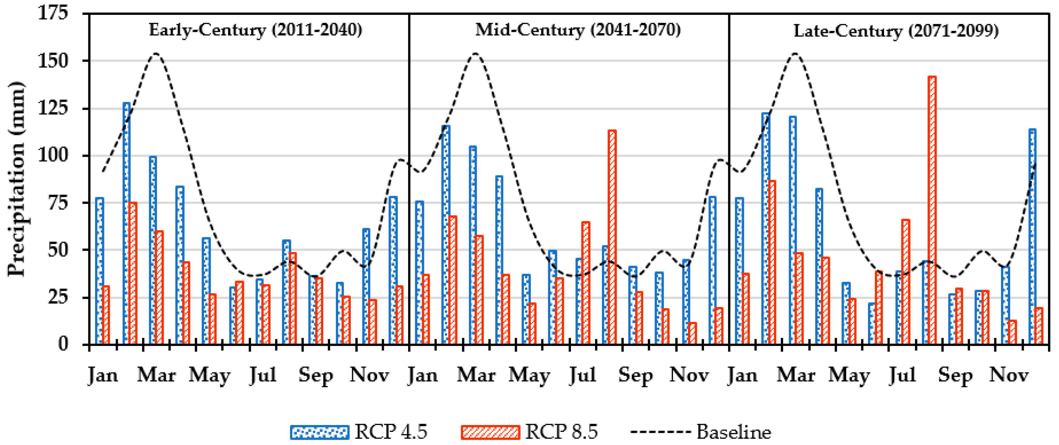
3.3.2. Precipitation

Precipitation is an important variable for the basin that has high sensitivity towards changing temperature. Therefore, the climate change study for both on annual and monthly scales are essential for deriving conclusive inferences. Annual precipitation (depicted in Figure S3) suggests extreme deviation and instability in precipitation quantities in case of RCP8.5 while projection by RCP4.5 remained somewhat stable overall. Nevertheless, an overall decrease in mean annual precipitation is estimated for both the scenarios during the entire 21st century. This decrease is more pronounced for spring and post-monsoon periods.

The monthly median precipitation depicts a shift in seasonal precipitation (Figure 5). The analysis further implies an overall reduction in precipitation in both the scenarios. However, intensity may vary and depends on the shifts in seasonal regime.

In case of RCP4.5, a monthly change in precipitation (

Table 6. Projected precipitation deviations (%) from baseline precipitation for RCP4.5 and RCP8.5 during early, mid, and late century.

Month	Jan	Feb	Mar	Apr	May	Jun	Jul	Aug	Sep	Oct	Nov	Dec
Baseline (mm)	91.89	121.48	154.22	114.96	64.89	40.15	36.91	43.97	35.98	49.56	42.95	96.22
RCP4.5
Early Century	−15.5	5.0	−35.6	−27.0	−13.0	−24.0	−5.6	24.9	1.6	−33.4	42.3	−18.5
Midcentury	−17.5	−4.7	−32.0	−22.4	−43.4	23.1	23.3	18.9	13.9	−23.3	4.8	−19.0
Late Century	−15.5	0.6	−22.0	−28.3	−49.7	−46.1	5.6	1.0	−25.7	−42.7	−3.8	18.7
Average	−16.15	+0.29	−29.88	−25.92	−35.33	−15.67	7.74	14.95	−3.42	−33.13	14.45	−6.29
RCP8.5
Early Century	−66.7	−38.3	−60.9	−61.8	−58.9	−17.2	−14.0	10.4	−1.6	−48.9	−44.3	−67.6
Midcentury	−59.8	−44.3	−62.5	−67.6	−66.8	−13.1	75.9	158.3	−22.5	−62.5	−73.8	−79.7
Late Century	−59.3	−28.5	−68.5	−60.0	−62.7	−3.9	78.5	221.9	−16.7	−42.9	−69.6	−79.6
Average	−61.89	−37.03	−63.98	−63.13	−62.78	−11.41	46.8	130.20	−13.60	−51.41	−62.59	−75.64

) shows winter precipitation (DJF) decreases below the historical baseline by up to −9.67%, reduction may continue until the midcentury, but thereafter a consistent increase up to 1.26% is projected during the late periods. The RCP8.5 scenario suggests high levels of reduction during winter, spring and dry seasons (DJF, MAM and SON) but it was able to demonstrate a higher increment of up to 98.84% during summer (JJA) during the late century. The overall total reduction of −15.94% and −35.05% corresponding to the baseline was estimated for RCP4.5 and RCP8.5, respectively, for the entire 21st century.

3.3.3. Water Availability

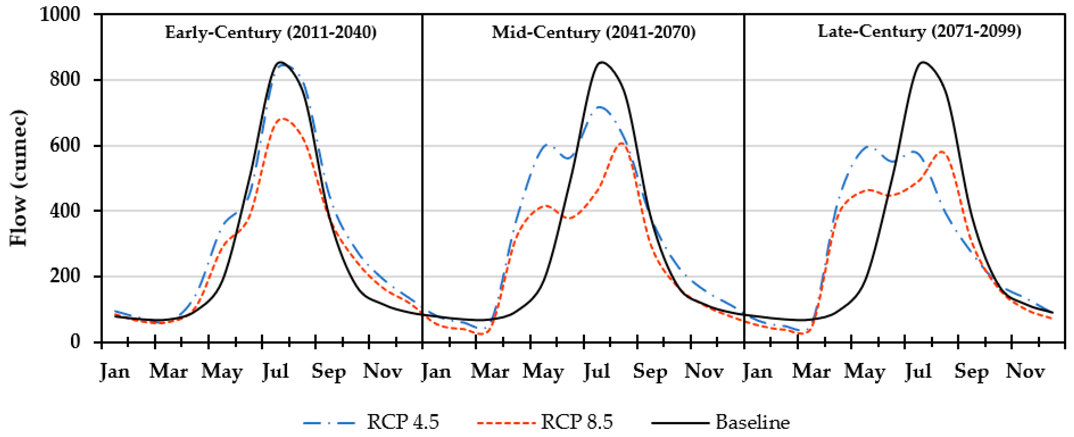
The climate variables have a tendency to intervene and affect the river flow regime of the basin; therefore, an appropriate analysis can provide the insight of variation brought by a changing climate. The mean annual flow analysis for both the historical and projection periods throughout the 21^st century is expressed in Figure S4. RCP4.5 shows a relatively smooth magnitude, the most extreme variation shown by a series is 483 cumec in 2028. On the other hand, the RCP8.5 flow series showed stochastic and high variation throughout the century.

The projected monthly median flows and the monthly percent change in the flow of future scenarios are shown in Figure S5 and

Table 7. Projected streamflow deviations (%) from baseline streamflow for RCP4.5 and RCP8.5 during early, mid, and late century.

Month	Jan	Feb	Mar	Apr	May	Jun	Jul	Aug	Sep	Oct	Nov	Dec
Baseline (m3/s)	77.64	68.78	68.47	94.52	187.31	496.51	846.61	767.12	380.32	171.21	114.91	89.6
RCP4.5
Early Century	19.83	3.60	−10.10	51.04	88.63	−9.77	−2.00	3.84	17.13	63.64	66.40	47.38
Midcentury	1.08	−15.18	−18.32	300.76	218.30	13.53	−15.41	−18.70	−0.14	34.93	36.52	23.81
Late Century	−17.26	−31.13	−23.64	357.26	216.44	10.91	−32.26	−48.63	−29.1	2.27	15.26	−2.69
Average	1.22	−14.24	−17.35	236.36	174.46	4.89	−16.56	−21.16	−4.04	33.61	39.39	22.83
RCP8.5
Early Century	9.65	−7.66	−9.32	13.77	54.46	−23.09	−21.14	−18.88	−0.84	44.09	44.01	32.80
Midcentury	−28.42	−41.00	−38.45	243.09	121.26	−23.85	−45.52	−21.50	−22.14	−1.21	−1.93	−12.60
Late Century	−33.06	−43.77	−33.80	311.01	146.36	−9.99	−42.00	−25.28	−20.84	−5.11	−12.51	−19.22
Average	−17.28	−30.81	−27.19	189.29	107.36	−18.98	−36.22	−21.89	−14.61	12.59	9.86	0.33

, respectively, corresponding to baseline flow in three intervals (early, mid, and late) of the 21st century. A flow analysis of RCP4.5 suggests an average rise of 14.33% in early century, while noticeable increments are estimated during MAM and SON months. Afterwards, the flow seems to depict a downward trajectory especially in the months of DJF, JJA, and SON except MAM where an extreme rise was observed. Nevertheless, at the end, flow tends to retain its magnitude almost equal to baseline. A rise up to +0.24% was detected for the RCP4.5 scenario during the late century. Overall a summary of the RCP4.5 scenario suggests a sudden rise in flow during the early century and a gradual decline during the rest of century. RCP8.5 showed almost similar dynamics to that of RCP4.5; however, the projected flow remained relatively less than RCP4.5. The analysis showed a decline in flow up to −6.82% for RCP8.5. Both scenarios depicted major increments in the months of April and May. While a major reduction was estimated during the months of July and August.

A major reduction in precipitation over the time and extreme rise in flow during April and May (seen in Table 7) implicitly suggests early melting of snow/glaciers in both scenarios.

3.3.4. Flow Regime

The Chitral River discharge has a strong correlation with precipitation and snow melt. These parameters are highly vulnerable to climate change which can cause changes in seasonal intensity and peak flows. Therefore, we considered studying changes in hydrological regime indicated by MIROC5_r1i1p1. Projected river flows depicted in Figure 6 suggest substantial shifts in monthly dynamics and magnitudes of the corresponding flows during the baseline period. Early century under RCP4.5 showed an adjacent rise in flows during the months of April until June. A slight rise was also detected during the recession months of September to December. Midcentury under a similar scenario shows the formation of two maxima due to a continuous rise in flow quantities during early summer in conjunction to a reduction in the former peak. Late century showed a somewhat similar pattern except the reduction in peak values during the month of July and early month peak became more pronounced. Changing patterns of hydrographs in the case of RCP8.5 are almost similar to that of RCP4.5 as both scenarios evolve to attain dual peak hydrographs. However, transition of RCP8.5 was much faster than RCP4.5 during this period. Overall, the projected result showed considerable shifts in peak flows values from midyear to the early spring season, which might be due to high snow/glacial melting as temperature rises.

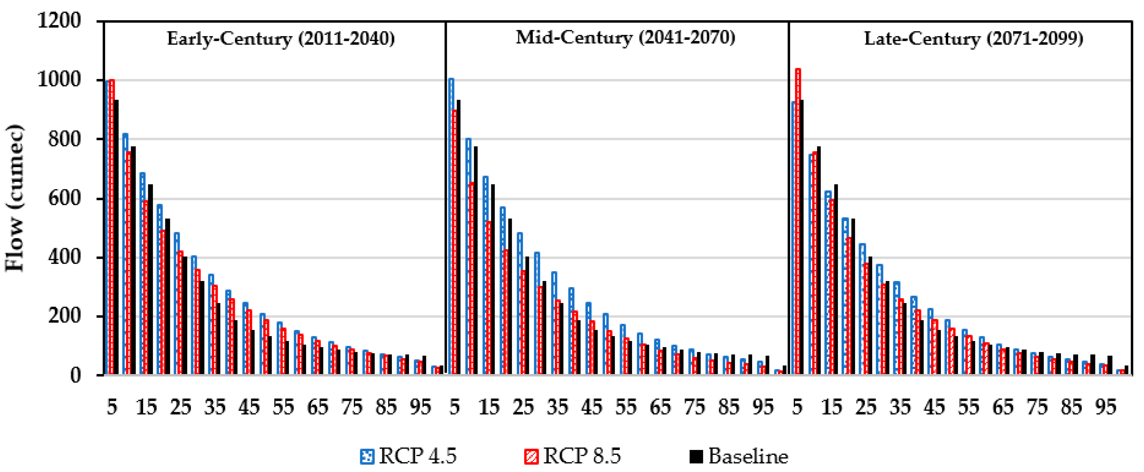
3.3.5. High and Low Flows

Water availability in terms of flow duration curve (FDC) is represented in Figure 7 to determine the duration of the two hydrological extremes of floods and droughts in the basin. The results represent the percentage of time period that a particular flow value is equaled or exceeded the mean values during the baseline period. The Y-axis shows the quantity of the flow at a given time associated with the duration, flow duration intervals are expressed as percentages of exceedance with (Q5 and Q10) denoting high stream discharge (floods) and (Q90 and Q100) as low stream discharge (drought) conditions, while the rest of the in-between interval is taken as a normal flow condition for convenience.

During the early century both scenarios showed a positive deviation from the baseline during high and normal flow conditions, with RCP4.5 attaining a higher magnitude overall. During the midcentury, reduction is evident in high flows in case of RCP8.5 while RCP4.5 retained its consistency. In the late century, the analysis indicates a decline in high flow for RCP4.5 whereas, normal flow condition remains almost similar. In the same period, RCP8.5 depicted a slight rise in normal flow conditions while a substantial rise in high flow suggests frequent flooding. Nevertheless, the analysis also suggests deficient quantities of low flow discharges for all scenarios implying frequent droughts.

4. Conclusions

This study appraises the anticipated future behavior of climate in the Chitral River Basin. Due to the lack of hydro-climatic stations and considerable systematic errors, precipitation estimations are less reliable and the retro-gridded datasets previously used have implications of their own. Therefore, this study emphasized the reliability of precipitation estimates and further chose ERA5 Land in compliance to research requirement. The stream flow was modeled through the state-of-the-art ARC-SWAT hydrological model and compared with observed river flows. After calibration, the model results showed better relationships than the uncalibrated model results with the observed stream flows. The obtained NSE and KGE values of calibration are 0.84 and 0.91 while backward and forward validation values ranged between 0.79 and 0.85 for the given parameters, values reflect that deviation of simulated mean and standard deviation are less than the mean and standard deviation of the observed data. Further, PBIAS, MAE, and RMSE values show lower biasness during the calibration period as compared with the validation period. Moreover, RMSE values remain less than the half of standard deviation of observation, which also showed good agreement.

The climate change studies were conducted for temperature, precipitation, and stream flow for the future scenario of RCP4.5 and RCP8.5. Century-wise (early, mid and late), future projections for temperature suggests an increment of (+1.28 °C, +2.92 °C, +3.67 °C) in minimum temperature (T_n) and (+1.10 °C, +2.96 °C and +3.81 °C) in maximum temperature (T_x) at RCP4.5. Similarly, the average T_n and T_x rise during three intervals of the 21st century are (1.44 °C, +6.30 °C, +6.21 °C) and (+0.15 °C, +2.76 °C, +5.03 °C) for the RCP8.5 scenario. Additionally, the analysis suggests T_n to be more profoundly affected by climate change than T_x especially in the case of RCP8.5. The rise in average temperature at end of the century was determined to be +3.73 °C and +5.62 °C for RCP4.5 and RCP8.5, respectively.

The precipitation analysis for scenarios advocates a decline in precipitation, almost up to −16% and −35% for RCP4.5 and RCP8.5, respectively, at the end of century. For RCP8.5, the projected winter precipitation declines up to −9.85% to account for the total year in contrast to summer which increases +28.85%.

Future projections of Chitral River flows suggest considerable shifts of peaks towards earlier months of April and May. Despite reduction in precipitation over the time, the flow rise during April and May implicitly suggests the extreme melting of snow in both scenarios. By the end of the century, the overall average flows suggest 0.25% rise for RCP4.5 and −6.82% decrease for RCP8.5 corresponding to the baseline scenario. Similarly, water availability by FDC suggests deficient quantities of water in RCP8.5 and slight surpluses in RCP4.5 during most of the year. On the other hand, a significant rise in frequency and intensity of high and low flows corresponding to baseline values for both the scenarios.

The analysis was able to provide an in-depth understanding of the relationship between the climate and hydrology of Chitral Basin. This research also implicitly attested the reliability of [7] dataset for hydrological modeling. Good results during statistical evaluation suggests successful implementation of that dataset. This emphasizes the necessity of the quality of the dataset in addition to its quantity. Apart from this, climate change results, discrepancies, and limitations highlighted during these studies must be properly dealt with for future studies. This study can contribute to formulate advance water resource management and engineering solutions for decision-making. Currently, various hydropower projects are underway as part of a government agenda. This research can provide guidance to these projects in terms of their design and operation.

References

1. Sabine, C. Ask the Experts: The IPCC Fifth Assessment Report. Carbon Manag. 2014, 5, 17–25. [Google Scholar] [CrossRef]
2. Lutz, A.; Immerzeel, W.W.; Kraaijenbrink, P.; Shrestha, A.; Bierkens, M.F.P. Climate Change Impacts on the Upper Indus Hydrology: Sources, Shifts and Extremes. PLoS ONE 2016, 11, e0165630. [Google Scholar] [CrossRef] [PubMed] [Green Version]
3. Ul Hasson, S.; Saeed, F.; Böhner, J.; Schleussner, C.-F. Water Availability in Pakistan from Hindukush-Karakoram-Himalayan Watersheds at 1.5 °C and 2 °C Paris Agreement Targets. Adv. Water Resour. 2019, 131, 103365. [Google Scholar] [CrossRef]
4. Hashmi, M.; Masood, A.; Mushtaq, H.; Bukhari, S.; Ahmad, B.; Tahir, A. Exploring Climate Change Impacts during the First Half of the 21st Century on Flow Regime of the Transboundary Kabul River in the Hindukush Region. J. Water Clim. Chang. 2019, 11, 1521–1538. [Google Scholar] [CrossRef]
5. Azmat, M.; Wahab, A.; Huggel, C.; Qamar, M.; Hussain, E.; Ahmad, S.; Waheed, A. Climatic and Hydrological Projections to Changing Climate under CORDEX-South Asia Experiments over the Karakoram-Hindukush-Himalayan Water Towers. Sci. Total Environ. 2019, 703, 135010. [Google Scholar] [CrossRef]
6. Aryal, J.; Jat, M.; Sapkota, T.; Khatri-Chhetri, A.; Kassie, M.; Rahut, D.B.; Maharjan, S. Adoption of Multiple Climate-Smart Agricultural Practices in the Gangetic Plains of Bihar, India. Int. J. Clim. Chang. Strateg. Manag. 2018, 10, 407–427. [Google Scholar] [CrossRef]
7. Dahri, Z.H.; Moors, E.; Ludwig, F.; Ahmad, S.; Khan, A.; Ali, I.; Kabat, P. Adjustment of Measurement Errors to Reconcile Precipitation Distribution in the High-Altitude Indus Basin. Int. J. Clim. 2018, 38, 3842–3860. [Google Scholar] [CrossRef]
8. Immerzeel, W.W.; Pellicciotti, F.; Bierkens, M.F.P. Rising River Flows throughout the Twenty-First Century in Two Himalayan Glacierized Watersheds. Nat. Geosci. 2013, 6, 742–745. [Google Scholar] [CrossRef]
9. Immerzeel, W.W.; Wanders, N.; Lutz, A.; Shea, J.M.; Bierkens, M.F.P. Reconciling High-Altitude Precipitation in the Upper Indus Basin with Glacier Mass Balances and Runoff. Hydrol. Earth Syst. Sci. 2015, 19, 4673–4687. [Google Scholar] [CrossRef] [Green Version]
10. Bokhari, S.; Ahmad, B.; Ali, J.; Ahmad, S.; Mushtaq, H.; Rasul, G. Future Climate Change Projections of the Kabul River Basin Using a Multi-Model Ensemble of High-Resolution Statistically Downscaled Data. Earth Syst. Environ. 2018, 2, 477–497. [Google Scholar] [CrossRef]
11. Lutz, A.; Immerzeel, W.W.; Shrestha, A.; Bierkens, M.F.P. Consistent Increase in High Asia’s Runoff Due to Increasing Glacier Melt and Precipitation. Nat. Clim. Chang. 2014, 4, 587–592. [Google Scholar] [CrossRef] [Green Version]
12. Nizami, A.; Ali, J.; Zulfiqar, M. Climate Change, Hydro-Meteorological Hazards and Adaptation for Sustainable Livelihood in Chitral Pakistan. Sarhad J. Agric. 2019, 35, 432–441. [Google Scholar] [CrossRef]
13. Ahmed, K.; Iqbal, Z.; Khan, N.; Rasheed, B.; Nawaz, N.; Malik, I.; Noor, M. Quantitative Assessment of Precipitation Changes under CMIP5 RCP Scenarios over the Northern Sub-Himalayan Region of Pakistan. Environ. Dev. Sustain. 2020, 22, 7831–7845. [Google Scholar] [CrossRef]
14. Ahmad, S.; Israr, M.; Liu, S.; Hayat, H.; Gul, J.; Wajid, S.; Ashraf, M.; Baig, S.; Tahir, A.; Gul, J. Spatio-Temporal Trends in Snow Extent and Their Linkage to Hydro-Climatological and Topographical Factors in the Chitral River Basin (Hindukush, Pakistan). Geocarto Int. 2018, 35, 711–734. [Google Scholar] [CrossRef]
15. Palazzi, E.; Hardenberg, J.; Provenzale, A. Precipitation in the Hindu-Kush Karakoram Himalaya: Observations and Future Scenarios. J. Geophys. Res. Atmos. 2013, 118, 85–100. [Google Scholar] [CrossRef]
16. Baudouin, J.-P.; Herzog, M.; Petrie, C. Cross-Validating Precipitation Datasets in the Indus River Basin. Hydrol. Earth Syst. Sci. 2019, 24, 427–450. [Google Scholar] [CrossRef] [Green Version]
17. Yuan, F.; Zhang, L.; Win, K.W.W.; Ren, L.; Zhao, C.; Zhu, Y.; Jiang, S.; Liu, Y. Assessment of GPM and TRMM Multi-Satellite Precipitation Products in Streamflow Simulations in a Data-Sparse Mountainous Watershed in Myanmar. Remote Sens. 2017, 9, 302. [Google Scholar] [CrossRef] [Green Version]
18. Iqbal, M.; Athar, H. Validation of Satellite Based Precipitation over Diverse Topography of Pakistan. Atmos. Res. 2017, 201, 247–260. [Google Scholar] [CrossRef]
19. Rana, S.; Mcgregor, J.; Renwick, J. Precipitation Seasonality over the Indian Subcontinent: An Evaluation of Gauge, Reanalyses and Satellite Retrievals. J. Hydrometeorol. 2014, 16, 631–651. [Google Scholar] [CrossRef]
20. Kishore, P.; Jyothi, S.; Basha, G.; Rao, S.; Rajeevan, M.; Velicogna, I.; Sutterley, T. Precipitation Climatology over India: Validation with Observations and Reanalysis Datasets and Spatial Trends. Clim. Dyn. 2015, 46, 541–556. [Google Scholar] [CrossRef] [Green Version]
21. Pelosi, A.; Terribile, F.; D’Urso, G.; Chirico, G.B. Comparison of ERA5-Land and UERRA MESCAN-SURFEX Reanalysis Data with Spatially Interpolated Weather Observations for the Regional Assessment of Reference Evapotranspiration. Water 2020, 12, 1669. [Google Scholar] [CrossRef]
22. Bromwich, D.; Wilson, A.; Bai, L.; Moore, G.W.K.; Bauer, P. A Comparison of the Regional Arctic System Reanalysis and the Global ERA-Interim Reanalysis for the Arctic. Q. J. R. Meteorol. Soc. 2015, 142, 644–658. [Google Scholar] [CrossRef] [Green Version]
23. Hersbach, H.; De Rosnay, P.; Bell, B.; Schepers, D.; Simmons, A.; Soci, C.; Abdalla, S.; Alonso-Balmaseda, M.; Balsamo, G.; Bechtold, P.; et al. Operational Global Reanalysis: Progress, Future Directions and Synergies with NWP; ERA Report Series No. 27; ECMWF: Reading, UK, 2018. [Google Scholar] [CrossRef]
24. Nesterova, N.; Makarieva, O.; Post, D.A. Parameterizing a Hydrological Model Using a Short-term Observational Dataset to Study Runoff Generation Processes and Reproduce Recent Trends in Streamflow at a Remote Mountainous Permafrost Basin. Hydrol. Process. 2021, 35, e14278. [Google Scholar] [CrossRef]
25. Dahri, Z.H.; Ludwig, F.; Moors, E.; Ahmad, S.; Ahmad, B.; Ahmad, S.; Riaz, M.; Kabat, P. Climate Change and Hydrological Regime of the High-Altitude Indus Basin under Extreme Climate Scenarios. Sci. Total Environ. 2021, 768, 144467. [Google Scholar] [CrossRef]
26. Ficklin, D.; Abatzoglou, J.; Robeson, S.; Dufficy, A. The Influence of Climate Model Biases on Projections of Aridity and Drought. J. Clim. 2015, 29, 1269–1285. [Google Scholar] [CrossRef]
27. Lutz, A.; ter Maat, H.; Biemans, H.; Shrestha, A.; Wester, P.; Immerzeel, W.W. Selecting Representative Climate Models for Climate Change Impact Studies: An Advanced Envelope-Based Selection Approach. Int. J. Climatol. 2016, 36, 3988–4005. [Google Scholar] [CrossRef] [Green Version]
28. Dahri, Z.H.; Ludwig, F.; Moors, E.; Ahmad, B.; Khan, A.; Kabat, P. An Appraisal of Precipitation Distribution in the High-Altitude Catchments of the Indus Basin. Sci. Total Environ. 2016, 548–549, 289–306. [Google Scholar] [CrossRef] [Green Version]
29. Hersbach, H.; Bell, B.; Berrisford, P.; Hirahara, S.; Horányi, A.; Muñoz-Sabater, J.; Nicolas, J.; Peubey, C.; Radu, R.; Schepers, D.; et al. The ERA5 Global Reanalysis. Q. J. R. Meteorol. Soc. 2020, 146, 1999–2049. [Google Scholar] [CrossRef]
30. ERA5-Land: Data Documentation. Available online: https://confluence.ecmwf.int/display/CKB/ERA5-Land%3A+data+documentation (accessed on 1 October 2021).
31. Copernicus Climate Change Service. ERA5-Land Hourly Data from 2001 to Present ECMWF. Available online: https://cds.climate.copernicus.eu/doi/10.24381/cds.e2161bac (accessed on 1 October 2021).
32. Shrestha, M.; Acharya, S.; Shrestha, P. Bias Correction of Climate Models for Hydrological Modeling—Are Simple Methods Still Useful? Meteorol. Appl. 2017, 24, 531–539. [Google Scholar] [CrossRef] [Green Version]
33. Teutschbein, C.; Seibert, J. Bias Correction of Regional Climate Model Simulations for Hydrological Climate-Change Impact Studies: Review and Evaluation of Different Methods. J. Hydrol. 2012, 456–457, 12–29. [Google Scholar] [CrossRef]
34. Lenderink, G.; van Ulden, A.; van den Hurk, B.; Keller, F. A Study on Combining Global and Regional Climate Model Results for Generating Climate Scenarios of Temperature and Precipitation for The Netherlands. Clim. Dyn. 2007, 29, 157–176. [Google Scholar] [CrossRef] [Green Version]
35. Arnold, J.; Srinivasan, R.; Muttiah, R.; Williams, J.R. Large Area Hydrologic Modeling and Assessment Part I: Model Development. JAWRA J. Am. Water Resour. Assoc. 1998, 34, 73–89. [Google Scholar] [CrossRef]
36. Gassman, P.; Sadeghi, A.; Srinivasan, R. Applications of the SWAT Model Special Section: Overview and Insights. J. Environ. Qual. 2014, 43, 1–8. [Google Scholar] [CrossRef] [PubMed]
37. Gassman, P.; Reyes, M.; Green, C.; Arnold, J. Soil and Water Assessment Tool: Historical Development, Applications, and Future Research Directions. Trans. ASABE 2007, 50, 1211–1250. [Google Scholar] [CrossRef] [Green Version]
38. Shrestha, S.; Shrestha, M.; Shrestha, P. Evaluation of the SWAT Model Performance for Simulating River Discharge in the Himalayan and Tropical Basins of Asia. Hydrol. Res. 2017, 49, 846–860. [Google Scholar] [CrossRef] [Green Version]
39. Neitsch, S.; Arnold, J.; Kinry, J.R.; Williams, J.R. Soil and Water Assessment Tool Theoretical Documentation Version 2009; TR-406; Texas Water Resources Institute: College Station, TX, USA, 2011. [Google Scholar]
40. FAO; IIASA; ISRIC; ISSCAS; JRC. Harmonized World Soil Database (Version 1.2); FAO: Rome, Italy; IIASA: Laxenburg, Austria, 2012. [Google Scholar]
41. Yang, J.; Reichert, P.; Abbaspour, K.C.; Xia, J.; Yang, H. Comparing Uncertainty Analysis Techniques for a SWAT Application to the Chaohe Basin in China. J. Hydrol. 2008, 358, 1–23. [Google Scholar] [CrossRef]
42. Ghoraba, S. Hydrological Modeling of the Simly Dam Watershed (Pakistan) Using GIS and SWAT Model. Alex. Eng. J. 2015, 54, 583–594. [Google Scholar] [CrossRef] [Green Version]
43. Abbaspour, K.C. SWATCalibration and Uncertainty Programs; Eawag: Dubendorf, Switzerland, 2015; 100p. [Google Scholar]
44. Abbaspour, K.C.; Ashraf Vaghefi, S.; Srinivasan, R. A Guideline for Successful Calibration and Uncertainty Analysis for Soil and Water Assessment: A Review of Papers from the 2016 International SWAT Conference. Water 2017, 10, 6. [Google Scholar] [CrossRef] [Green Version]
45. Hosseini, S.H.; Hashemi, H.; Fakheri Fard, A.; Berndtsson, R. Areal Precipitation Coverage Ratio for Enhanced AI Modelling of Monthly Runoff: A New Satellite Data-Driven Scheme for Semi-Arid Mountainous Climate. Remote Sens. 2022, 14, 270. [Google Scholar] [CrossRef]
Figure 1. Location map of the Chitral River Basin.
Atmosphere 13 00295 g001
Figure 2. (a) Land cover and (b) soil classifications in the Chitral River Basin.
Atmosphere 13 00295 g002
Figure 3. Daily simulated and observed flows during calibration and validation periods.
Atmosphere 13 00295 g003
Figure 4. Comparisons of the baseline maximum and minimum temperatures (Tx, Tn) with the projected temperatures for RCP4.5 and RCP8.5 during early, mid, and late century.
Atmosphere 13 00295 g004
Figure 5. Comparison of the baseline precipitation with the projected precipitation for RCP4.5 and RCP8.5 during early, mid, and late century.
Atmosphere 13 00295 g005
Figure 6. Flow regime, shifts in seasonality and annual cycle of hydrological peaks for RCP4.5, and RCP8.5 during early, mid, and late century.
Atmosphere 13 00295 g006
Figure 7. Comparison of 21st century water availability with baseline for RCP4.5 and RCP8.5 during early, mid, and late century.
Atmosphere 13 00295 g007