
Spatiotemporal Patterns and Regional Transport of Ground-Level Ozone in Major Urban Agglomerations in China

 , , ,
, , , 
Abstract
:1. Introduction
2. Data and Methods
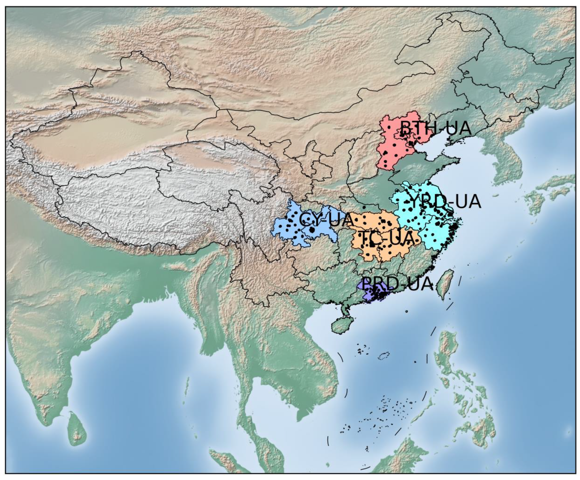
2.1. Study Area
2.2. Data Source and Description
2.3. Spatiotemporal Variation Analysis Methods
2.3.1. Kernel-Density Estimation
2.3.2. Empirical Orthogonal Function Analysis
2.3.3. Standard Deviational Ellipse
2.3.4. Global and Local Spatial Autocorrelation Analysis
2.4. Regional Background Estimated and Pollution Source Analysis
2.4.1. Texas Commission on Environmental Quality Method
2.4.2. Kolmogorov–Zurbenko Filter
2.4.3. Backward Trajectory
2.4.4. Potential Source Analysis
3. Temporal Variations of O3 in Five Urban Agglomerations
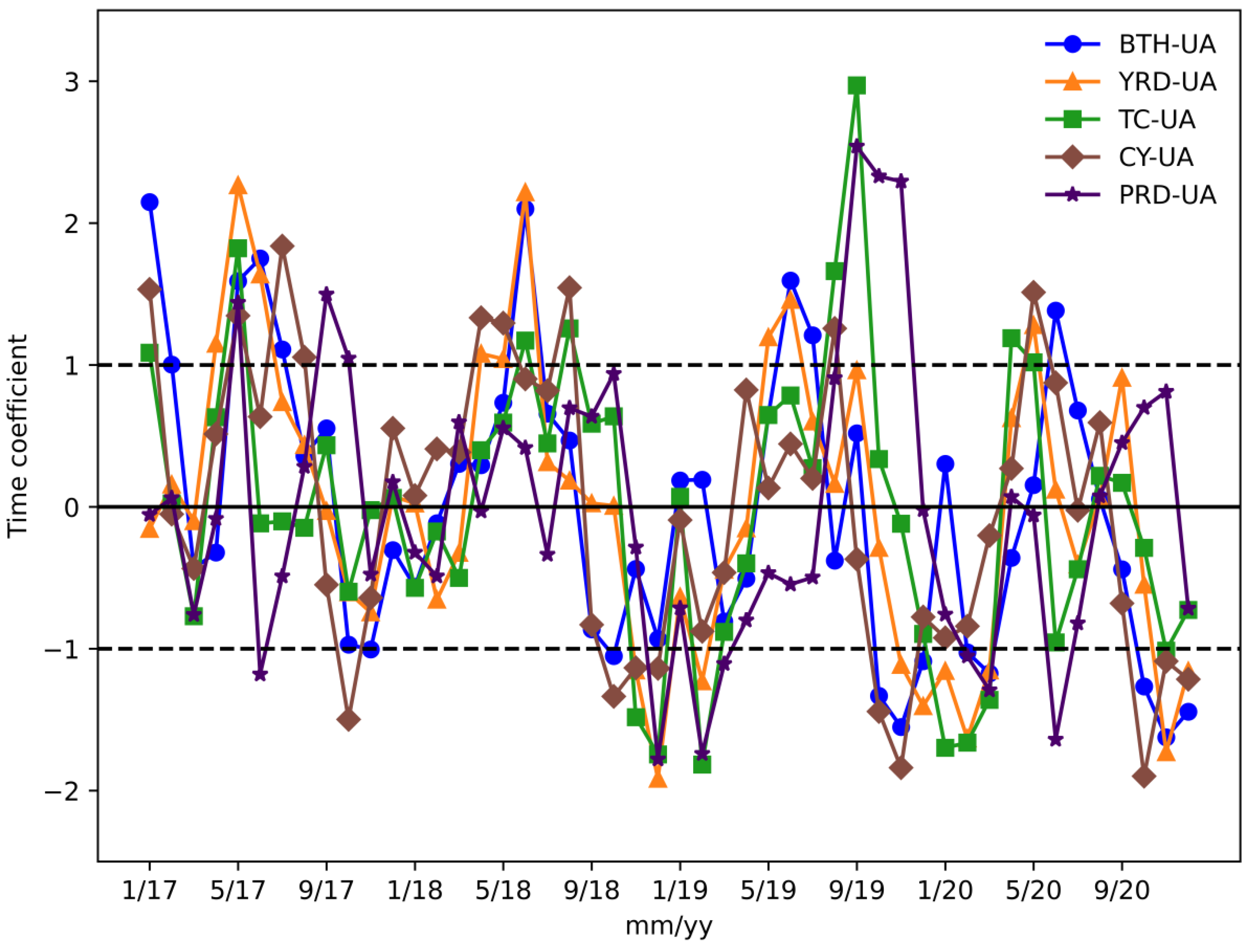
3.1. Annual Variation
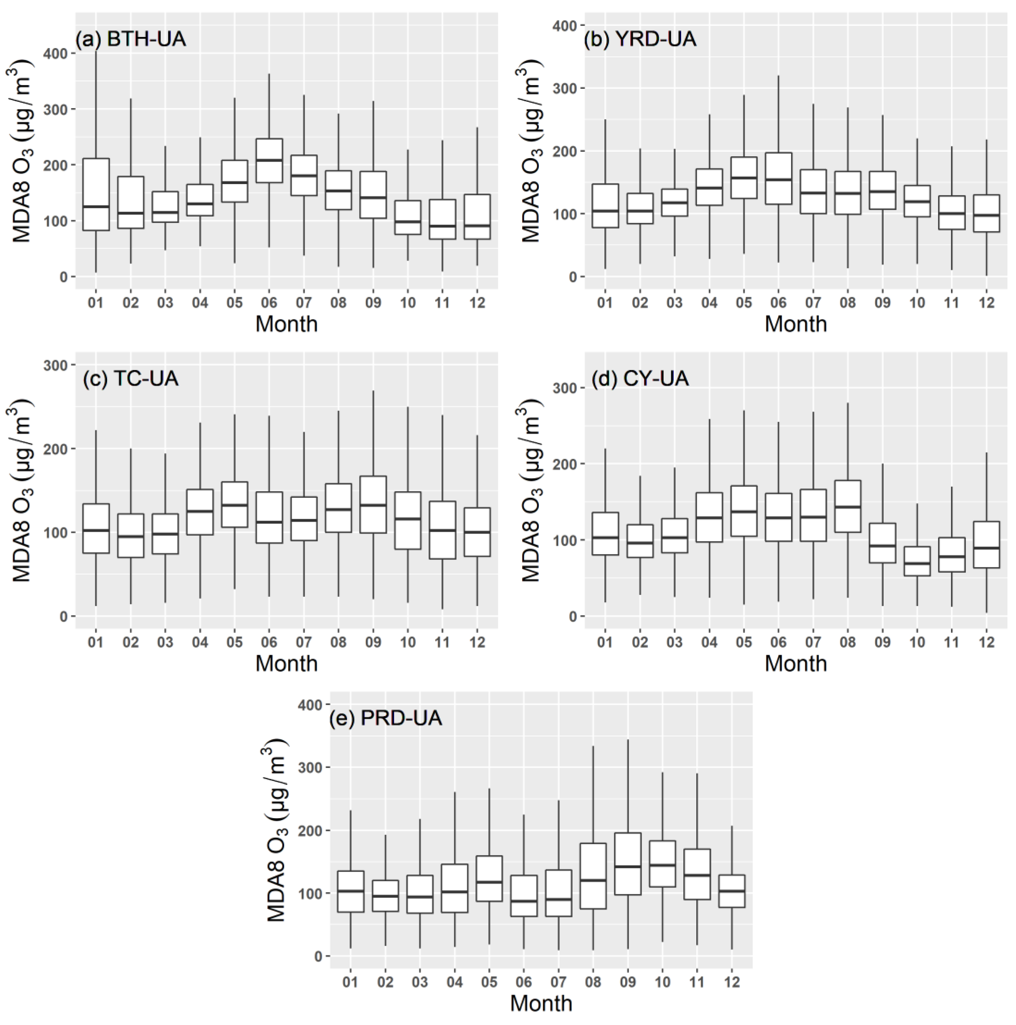
3.2. Monthly Variation
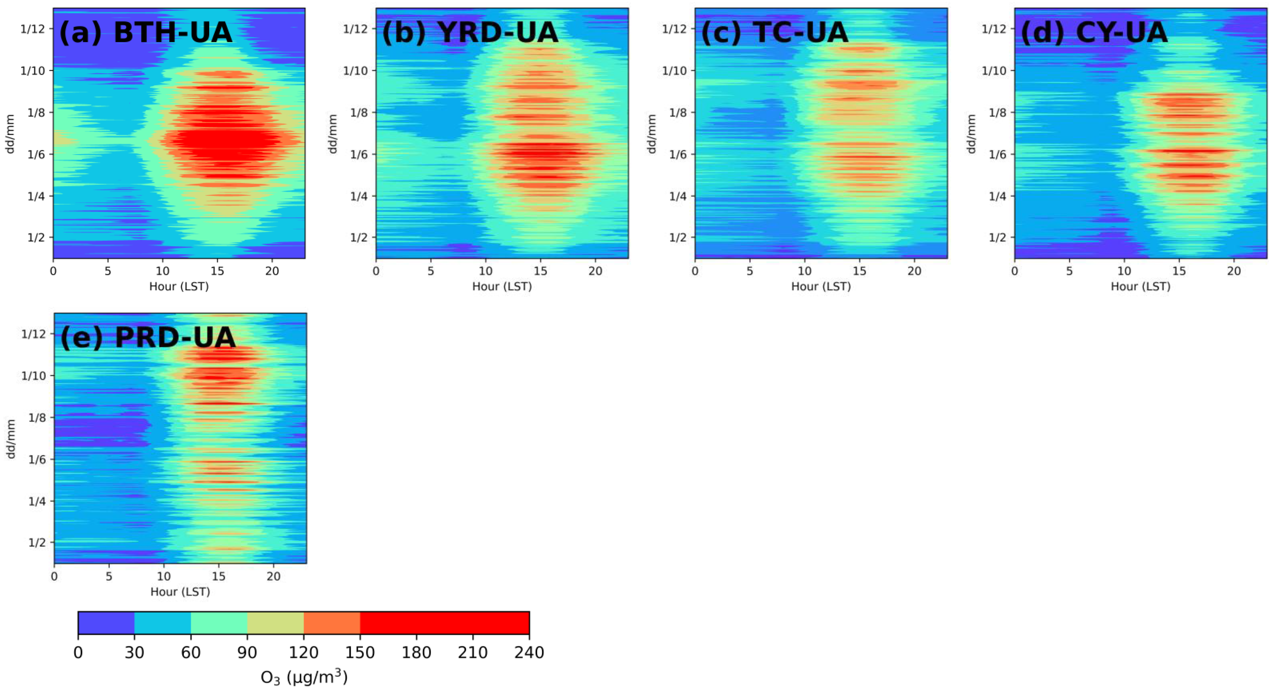
3.3. Diurnal Variation
4. Spatial Variations of O3 in Five Urban Agglomerations
4.1. Standard Deviational Ellipse Analysis
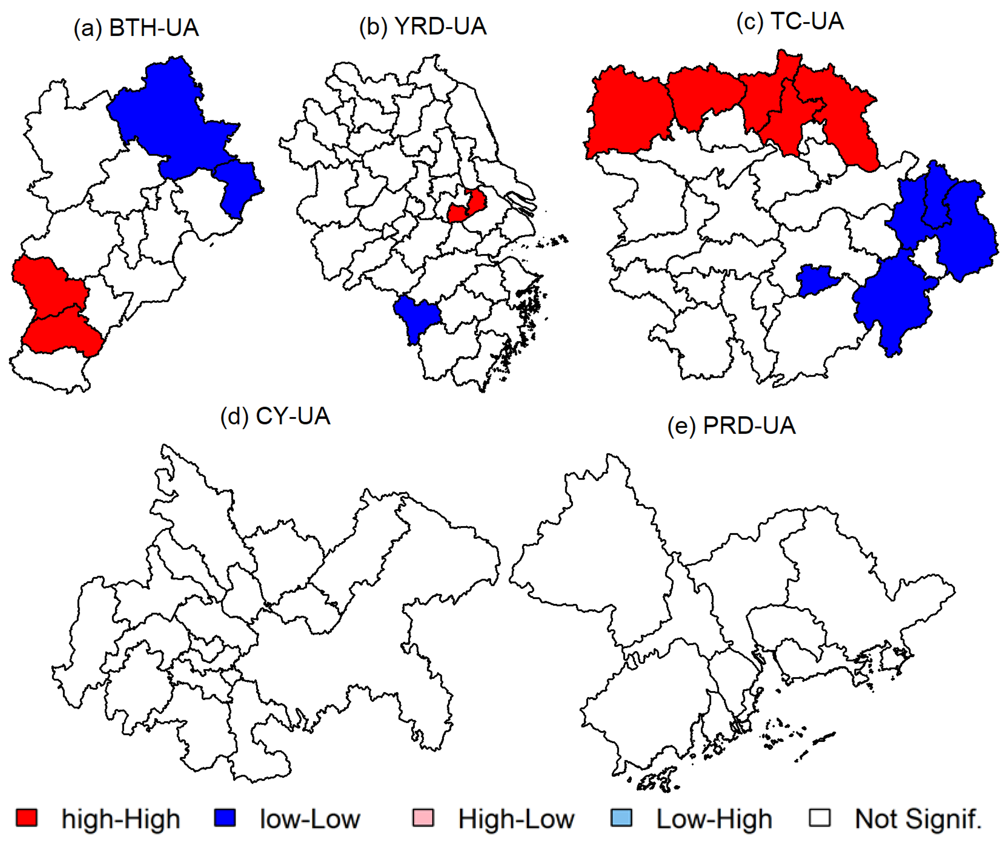
4.2. Spatial Autocorrelation of O3 Concentrations
5. Regional Transport of O3 in Five Typical Cities
5.1. O3 Time Series Separated by KZ Filter
5.2. Backward Trajectory Analysis
5.3. Potential Sources
6. Conclusions
Supplementary Materials
Author Contributions
Funding
Institutional Review Board Statement
Informed Consent Statement
Data Availability Statement
Acknowledgments
Conflicts of Interest
References
- Huang, R.J.; Zhang, Y.L.; Bozzetti, C.; Ho, K.F.; Cao, J.J.; Han, Y.M.; Daellenbach, K.R.; Slowik, J.G.; Platt, S.M.; Canonaco, F.; et al. High secondary aerosol contribution to particulate pollution during haze events in China. Nature 2014, 514, 218–222. [Google Scholar] [CrossRef] [PubMed] [Green Version]
- Zhao, S.; Yin, D.; Yu, Y.; Kang, S.; Qin, D.; Dong, L. PM2.5 and O3 pollution during 2015–2019 over 367 Chinese cities: Spatiotemporal variations, meteorological and topographical impacts. Environ. Pollut. 2020, 264, 114694. [Google Scholar] [CrossRef] [PubMed]
- Liu, X.Y.; Wang, M.S.; Pan, X.L.; Wang, X.Y.; Yue, X.L.; Zhang, D.H.; Ma, Z.G.; Tian, Y.; Liu, H.; Lei, S.D.; et al. Chemical formation and source apportionment of PM2.5 at an urban site at the southern foot of the Taihang mountains. J. Environ. Sci. 2021, 103, 20–32. [Google Scholar] [CrossRef] [PubMed]
- Lu, H.; Lyu, X.; Cheng, H.; Ling, Z.; Guo, H. Overview on the spatial-temporal characteristics of the ozone formation regime in China. Environ. Sci. Process. Impacts 2019, 21, 916–929. [Google Scholar] [CrossRef] [PubMed]
- Fang, T.; Zhu, Y.; Wang, S.; Xing, J.; Zhao, B.; Fan, S.; Li, M.; Yang, W.; Chen, Y.; Huang, R. Source impact and contribution analysis of ambient ozone using multi-modeling approaches over the Pearl River Delta region, China. Environ. Pollut. 2021, 289, 117860. [Google Scholar] [CrossRef] [PubMed]
- Wei, J.; Li, Z.; Lyapustin, A.; Sun, L.; Peng, Y.; Xue, W.; Su, T.; Cribb, M. Reconstructing 1-km-resolution high-quality PM2.5 data records from 2000 to 2018 in China: Spatiotemporal variations and policy implications. Remote Sens. Environ. 2021, 252, 112136. [Google Scholar] [CrossRef]
- Wang, Z.S.; Lv, J.G.; Tan, Y.F.; Guo, M.; Gu, Y.Y.; Xu, S.; Zhou, Y.H. Temporospatial variations and Spearman correlation analysis of ozone concentrations to nitrogen dioxide, sulfur dioxide, particulate matters and carbon monoxide in ambient air, China. Atmos. Pollut. Res. 2019, 10, 1203–1210. [Google Scholar] [CrossRef]
- Wei, J.; Li, Z.; Li, K.; Dickerson, R.R.; Pinker, R.T.; Wang, J.; Liu, X.; Sun, L.; Xue, W.; Cribb, M. Full-coverage mapping and spatiotemporal variations of ground-level ozone (O3) pollution from 2013 to 2020 across China. Remote Sens. Environ. 2022, 270, 112775. [Google Scholar] [CrossRef]
- Wang, C.L.; Wang, Y.Y.; Shi, Z.H.; Sun, J.J.; Gong, K.J.; Li, J.Y.; Qin, M.M.; Wei, J.; Li, T.T.; Kan, H.D.; et al. Effects of using different exposure data to estimate changes in premature mortality attributable to PM2.5 and O3 in China. Environ. Pollut. 2021, 285, 117242. [Google Scholar] [CrossRef]
- Liu, J.; Yin, H.; Tang, X.; Zhu, T.; Zhang, Q.; Liu, Z.; Tang, X.L.; Yi, H.H. Transition in air pollution, disease burden and health cost in China: A comparative study of long-term and short-term exposure. Environ. Pollut. 2021, 277, 116770. [Google Scholar] [CrossRef]
- Ren, J.Z. Effects of O3 pollution near formation on crop yield and economic loss. Environ. Technol. Innov. 2021, 22, 101446. [Google Scholar] [CrossRef]
- Cao, J.C.; Wang, X.M.; Zhao, H.; Ma, M.R.; Chang, M. Evaluating the effects of ground-level O3 on rice yield and economic losses in southern China. Environ. Pollut. 2020, 267, 115694. [Google Scholar] [CrossRef] [PubMed]
- Zhao, H.; Chen, K.Y.; Liu, Z.; Zhang, Y.X.; Shao, T.; Zhang, H.L. Coordinated control of PM2.5 and O3 is urgently needed in China after implementation of the “air pollution prevention and control action plan”. Chemosphere 2021, 270, 129441. [Google Scholar] [CrossRef] [PubMed]
- Chen, Y.Y.; Bai, Y.; Liu, H.T.; Alatalo, J.M.; Jiang, B. Temporal variations in ambient air quality indicators in Shanghai municipality, China. Sci. Rep. 2020, 10, 11350. [Google Scholar] [CrossRef] [PubMed]
- He, G.W.; Deng, T.; Wu, D.; Wu, C.; Huang, X.F.; Li, Z.N.; Yin, C.Q.; Zou, Y.; Song, L.; Ouyang, S.S.; et al. Characteristics of boundary layer ozone and its effect on surface ozone concentration in Shenzhen, China: A case study. Sci. Total Environ. 2021, 791, 148044. [Google Scholar] [CrossRef] [PubMed]
- Yang, X.Y.; Wu, K.; Wang, H.L.; Liu, Y.M.; Gu, S.; Lu, Y.Q.; Zhang, X.L.; Hu, Y.S.; Ou, Y.H.; Wang, S.G.; et al. Summertime ozone pollution in Sichuan basin, China: Meteorological conditions, sources and process analysis. Atmos. Environ. 2020, 226, 117392. [Google Scholar] [CrossRef]
- Ma, X.; Jia, H.; Sha, T.; An, J.; Tian, R. Spatial and seasonal characteristics of particulate matter and gaseous pollution in China: Implications for control policy. Environ. Pollut. 2019, 248, 421–428. [Google Scholar] [CrossRef]
- Li, R.; Wang, Z.Z.; Cui, L.L.; Fu, H.B.; Zhang, L.W.; Kong, L.D.; Chen, W.D.; Chen, J.M. Air pollution characteristics in China during 2015-2016: Spatiotemporal variations and key meteorological factors. Sci. Total Environ. 2019, 648, 902–915. [Google Scholar] [CrossRef]
- Suciu, L.G.; Griffin, R.J.; Masiello, C.A. Regional background O3 and NOx in the Houston-Galveston-Brazoria (TX) region: A decadal-scale perspective. Atmos. Chem. Phys. 2017, 17, 6565–6581. [Google Scholar] [CrossRef] [Green Version]
- Gong, K.J.; Li, L.; Li, J.Y.; Qin, M.M.; Wang, X.Y.; Ying, Q.; Liao, H.; Guo, S.; Hu, M.; Zhang, Y.H.; et al. Quantifying the impacts of inter-city transport on air quality in the Yangtze River Delta urban agglomeration, China: Implications for regional cooperative controls of PM2.5 and O3. Sci. Total Environ. 2021, 779, 146619. [Google Scholar] [CrossRef]
- Wang, M.Y.; Yim, S.H.L.; Dong, G.H.; Ho, K.F.; Wong, D.C. Mapping ozone source-receptor relationship and apportioning the health impact in the Pearl River Delta region using adjoint sensitivity analysis. Atmos. Environ. 2020, 222, 117026. [Google Scholar] [CrossRef] [PubMed]
- Li, L.; An, J.Y.; Huang, L.; Yan, R.S.; Huang, C.; Yarwood, R. Ozone source apportionment over the Yangtze River Delta region, China: Investigation of regional transport, sectoral contributions and seasonal differences. Atmos. Environ. 2019, 202, 269–280. [Google Scholar] [CrossRef]
- Zhang, X.; Jin, Y.N.; Dai, H.C.; Xie, Y.; Zhang, S.Q. Health and economic benefits of cleaner residential heating in the Beijing-Tianjin-Hebei region in China. Energy Policy 2019, 127, 165–178. [Google Scholar] [CrossRef]
- Shen, Y.; Zhang, L.P.; Fang, X.; Ji, H.Y.; Li, X.; Zhao, Z.W. Spatiotemporal patterns of recent PM2.5 concentrations over typical urban agglomerations in China. Sci. Total Environ. 2019, 655, 13–26. [Google Scholar] [CrossRef]
- Ma, T.; Duan, F.K.; He, K.B.; Qin, Y.; Tong, D.; Geng, G.N.; Liu, X.Y.; Li, H.; Yang, S.; Ye, S.Q.; et al. Air pollution characteristics and their relationship with emissions and meteorology in the Yangtze River Delta region during 2014-2016. J. Environ. Sci. 2019, 83, 8–20. [Google Scholar] [CrossRef]
- Sun, X.W.; Cheng, S.Y.; Lang, J.L.; Ren, Z.H.; Sun, C. Development of emissions inventory and identification of sources for priority control in the middle reaches of Yangtze River urban agglomerations. Sci. Total Environ. 2018, 625, 155–167. [Google Scholar] [CrossRef]
- Liao, T.T.; Wang, S.; Ai, J.; Gui, K.; Duan, B.L.; Zhao, Q.; Zhang, X.; Jiang, W.T.; Sun, Y. Heavy pollution episodes, transport pathways and potential sources of PM2.5 during the winter of 2013 in Chengdu (China). Sci. Total Environ. 2017, 584, 1056–1065. [Google Scholar] [CrossRef]
- Cheng, L.J.; Wang, S.; Gong, Z.Y.; Li, H.; Yang, Q.; Wang, Y.Y. Regionalization based on spatial and seasonal variation in ground-level ozone concentrations across China. J. Environ. Sci. 2018, 67, 179–190. [Google Scholar] [CrossRef] [Green Version]
- Yang, G.F.; Liu, Y.H.; Li, X.N. Spatiotemporal distribution of ground-level ozone in China at a city level. Sci. Rep. 2020, 10, 7229. [Google Scholar] [CrossRef]
- Jiang, L.; He, S.X.; Zhou, H.F. Spatio-temporal characteristics and convergence trends of PM2.5 pollution: A case study of cities of air pollution transmission channel in Beijing-Tianjin-Hebei region, China. J. Clean. Prod. 2020, 256, 120631. [Google Scholar] [CrossRef]
- Liu, Y.; Shi, G.; Zhan, Y.; Zhou, L.; Yang, F. Characteristics of PM2.5 spatial distribution and influencing meteorological conditions in Sichuan basin, southwestern China. Atmos. Environ. 2021, 253, 118364. [Google Scholar] [CrossRef]
- Xu, H.; Xiao, Z.M.; Chen, K.; Tang, M.; Zheng, N.Y.; Li, P.; Yang, N.; Yang, W.; Deng, X.W. Spatial and temporal distribution, chemical characteristics, and sources of ambient particulate matter in the Beijing-Tianjin-Hebei region. Sci. Total Environ. 2019, 658, 280–293. [Google Scholar] [CrossRef] [PubMed]
- Shi, Y.; Matsunaga, T.; Yamaguchi, Y.; Zhao, A.; Li, Z.; Gu, X. Long-term trends and spatial patterns of PM2.5-induced premature mortality in south and southeast Asia from 1999 to 2014. Sci. Total Environ. 2018, 631–632, 1504–1514. [Google Scholar] [CrossRef] [PubMed]
- Wachowicz, M.; Liu, T.Y. Finding spatial outliers in collective mobility patterns coupled with social ties. Int. J. Geogr. Inf. Sci. 2016, 30, 1806–1831. [Google Scholar] [CrossRef]
- Ye, W.F.; Ma, Z.Y.; Ha, X.Z. Spatial-temporal patterns of PM2.5 concentrations for 338 Chinese cities. Sci. Total Environ. 2018, 631–632, 524–533. [Google Scholar] [CrossRef]
- Wu, X.; Ding, Y.; Zhou, S.; Tan, Y. Temporal characteristic and source analysis of PM2.5 in the most polluted city agglomeration of China. Atmos. Pollut. Res. 2018, 9, 1221–1230. [Google Scholar] [CrossRef]
- Berlin, S.R.; Langford, A.O.; Estes, M.; Dong, M.; Parrish, D.D. Magnitude, decadal changes, and impact of regional background ozone transported into the greater Houston, Texas, area. Environ. Sci. Technol. 2013, 47, 13985–13992. [Google Scholar] [CrossRef]
- Nielson-Gammon, J.; Tobin, J.; Mcneel, A.; Li, G. A Conceptual Model. for Eight-Hour Ozone Exceedances in Houston, Texas Part. I: Background Ozone Levels in Eastern Texas; Texas A&M University: College Station, TX, USA, 2005. [Google Scholar]
- Rao, S.T.; Zalewsky, E.; Zurbenko, I.G. Determining temporal and spatial variations in ozone air quality. J. Air Waste Manag. Assoc. 1995, 45, 57–61. [Google Scholar] [CrossRef]
- Ma, Z.Q.; Xu, J.; Quan, W.J.; Zhang, Z.Y.; Lin, W.L.; Xu, X.B. Significant increase of surface ozone at a rural site, north of eastern China. Atmos. Chem. Phys. 2016, 16, 3969–3977. [Google Scholar] [CrossRef] [Green Version]
- Rao, S.T.; Zurbenko, I.G. Detecting and tracking changes in ozone air quality. J. Air Waste Manag. Assoc. 1994, 44, 1089–1092. [Google Scholar] [CrossRef]
- Agudelo-Castaneda, D.M.; Teixeira, E.C.; Pereira, F.N. Time-series analysis of surface ozone and nitrogen oxides concentrations in an urban area at Brazil. Atmos. Pollut. Res. 2014, 5, 411–420. [Google Scholar] [CrossRef] [Green Version]
- Li, P.; Wang, Y.; Dong, Q. The analysis and application of a new hybrid pollutants forecasting model using modified Kolmogorov-Zurbenko filter. Sci. Total Environ. 2017, 583, 228–240. [Google Scholar] [CrossRef] [PubMed]
- Wise, E.K.; Comrie, A.C. Extending the Kolmogorov-Zurbenko filter: Application to ozone, particulate matter, and meteorological trends. J. Air Waste Manag. Assoc. 2005, 55, 1208–1216. [Google Scholar] [CrossRef] [PubMed]
- Zhang, Z.Y.; Wong, M.S.; Lee, K.H. Estimation of potential source regions of PM2.5 in Beijing using backward trajectories. Atmos. Pollut. Res. 2015, 6, 173–177. [Google Scholar] [CrossRef] [Green Version]
- Zhao, S.P.; Yin, D.Y.; Qu, J.J. Identifying sources of dust based on Calipso, Modis satellite data and backward trajectory model. Atmos. Pollut. Res. 2015, 6, 36–44. [Google Scholar] [CrossRef] [Green Version]
- Stein, A.F.; Draxler, R.R.; Rolph, G.D.; Stunder, B.J.B.; Cohen, M.D.; Ngan, F. Noaa’s Hysplit atmospheric transport and dispersion modeling system. Bull. Am. Meteorol. Soc. 2015, 96, 2059–2077. [Google Scholar] [CrossRef]
- Liu, X.Y.; Pan, X.L.; Wang, Z.F.; He, H.; Wang, D.W.; Liu, H.; Tian, Y.; Xiang, W.L.; Li, J. Chemical characteristics and potential sources of PM2.5 in Shahe city during severe haze pollution episodes in the winter. Aerosol Air Qual. Res. 2020, 20, 2741–2753. [Google Scholar] [CrossRef]
- Xu, X.M.; Zhang, W.; Zhu, C.; Li, J.R.; Yuan, W.P.; Lv, J.L. Regional sources and the economic cost assessment of PM2.5 in Ji’nan, eastern China. Atmos. Pollut. Res. 2021, 12, 386–394. [Google Scholar] [CrossRef]
- Zhang, C.; Liu, X.G.; Zhang, Y.Y.; Tan, Q.W.; Feng, M.; Qu, Y.; An, J.L.; Deng, Y.J.; Zhai, R.X.; Wang, Z.; et al. Characteristics, source apportionment and chemical conversions of VOCs based on a comprehensive summer observation experiment in Beijing. Atmos. Pollut. Res. 2021, 12, 183–194. [Google Scholar] [CrossRef]
- Zhang, Q.; Yuan, B.; Shao, M.; Wang, X.; Lu, S.; Lu, K.; Wang, M.; Chen, L.; Chang, C.C.; Liu, S.C. Variations of ground-level O3 and its precursors in Beijing in summertime between 2005 and 2011. Atmos. Chem. Phys. 2014, 14, 6089–6101. [Google Scholar] [CrossRef] [Green Version]
- Yin, C.Q.; Solmon, F.; Deng, X.J.; Zou, Y.; Deng, T.; Wang, N.; Li, F.; Mai, B.R.; Liu, L. Geographical distribution of ozone seasonality over China. Sci. Total Environ. 2019, 689, 625–633. [Google Scholar] [CrossRef] [PubMed]
- Zhao, S.P.; Yu, Y.; Yin, D.Y.; He, J.J.; Liu, N.; Qu, J.J.; Xiao, J.H. Annual and diurnal variations of gaseous and particulate pollutants in 31 provincial capital cities based on in situ air quality monitoring data from China national environmental monitoring center. Environ. Int. 2016, 86, 92–106. [Google Scholar] [CrossRef] [PubMed]
- Yang, L.; Xie, D.; Yuan, Z.; Huang, Z.; Wu, H.; Han, J.; Liu, L.; Jia, W. Quantification of regional ozone pollution characteristics and its temporal evolution: Insights from identification of the impacts of meteorological conditions and emissions. Atmosphere 2021, 12, 279. [Google Scholar] [CrossRef]
- Zhang, A.; Lin, J.; Chen, W.; Lin, M.; Lei, C. Spatial-temporal distribution variation of ground-level ozone in China’s Pearl River Delta metropolitan region. Int. J. Environ. Res. Public Health 2021, 18, 872. [Google Scholar] [CrossRef]
- Wang, T.; Xue, L.; Brimblecombe, P.; Lam, Y.F.; Li, L.; Zhang, L. Ozone pollution in China: A review of concentrations, meteorological influences, chemical precursors, and effects. Sci. Total Environ. 2017, 575, 1582–1596. [Google Scholar] [CrossRef]


| Region | Year | Season | ||||||
|---|---|---|---|---|---|---|---|---|
| 2017 | 2018 | 2019 | 2020 | Spring | Summer | Autumn | Winter | |
| BTH-UA | 1.74 | 1.94 | 2.04 | 2.15 | 1.63 | 0.89 | 1.74 | 2.41 |
| YRD-UA | 0.16 | 0.10 | 0.43 | 0.44 | 2.27 | 2.04 | 2.15 | 3.19 |
| TC-UA | 1.20 | 2.50 | 2.46 | 1.69 | 1.69 | 2.57 | 0.37 | 2.37 |
| CY-UA | −0.72 | −0.29 | −0.59 | −0.21 | −0.54 | −0.29 | −0.49 | −0.13 |
| PRD-UA | 0.16 | −0.47 | −1.01 | −0.67 | −0.27 | 0.32 | 1.31 | −0.11 |
| City | D(W) | D(S) | D(e) | K |
|---|---|---|---|---|
| Beijing | 36.6% | 63.1% | 0.2% | 4.4% |
| Shanghai | 59.6% | 38.5% | 1.9% | 5.9% |
| Wuhan | 46.4% | 53.3% | 0.3% | 6.3% |
| Chengdu | 39.1% | 59.9% | 0.9% | 5.1% |
| Shenzhen | 68.8% | 30.9% | 0.3% | 9.0% |
Publisher’s Note: MDPI stays neutral with regard to jurisdictional claims in published maps and institutional affiliations. |
© 2022 by the authors. Licensee MDPI, Basel, Switzerland. This article is an open access article distributed under the terms and conditions of the Creative Commons Attribution (CC BY) license (https://creativecommons.org/licenses/by/4.0/).
Share and Cite
Liu, X.; Zhao, C.; Niu, J.; Su, F.; Yao, D.; Xu, F.; Yan, J.; Shen, X.; Jin, T. Spatiotemporal Patterns and Regional Transport of Ground-Level Ozone in Major Urban Agglomerations in China. Atmosphere 2022, 13, 301. https://doi.org/10.3390/atmos13020301
Liu X, Zhao C, Niu J, Su F, Yao D, Xu F, Yan J, Shen X, Jin T. Spatiotemporal Patterns and Regional Transport of Ground-Level Ozone in Major Urban Agglomerations in China. Atmosphere. 2022; 13(2):301. https://doi.org/10.3390/atmos13020301
Chicago/Turabian StyleLiu, Xiaoyong, Chengmei Zhao, Jiqiang Niu, Fangcheng Su, Dan Yao, Feng Xu, Junhui Yan, Xinzhi Shen, and Tao Jin. 2022. "Spatiotemporal Patterns and Regional Transport of Ground-Level Ozone in Major Urban Agglomerations in China" Atmosphere 13, no. 2: 301. https://doi.org/10.3390/atmos13020301
APA StyleLiu, X., Zhao, C., Niu, J., Su, F., Yao, D., Xu, F., Yan, J., Shen, X., & Jin, T. (2022). Spatiotemporal Patterns and Regional Transport of Ground-Level Ozone in Major Urban Agglomerations in China. Atmosphere, 13(2), 301. https://doi.org/10.3390/atmos13020301