Projection of the Near-Future PM_2.5 in Northern Peninsular Southeast Asia under RCP8.5

Abstract

Throughout the year, particularly during the dry season, the northern peninsula of Southeast Asia struggles with air pollution from PM_2.5. In this study, we used the Nested Regional Climate and Chemistry Model (NRCM-Chem) to predict the PM_2.5 concentrations over Southeast Asia’s northern peninsula during the years 2020–2029 under the Representative Concentration Pathway (RCP)8.5. In general, the model reasonably shows a good result, including temperature, precipitation, and PM_2.5 concentration, compared to the observation with an Index of Agreement (IOA) in the range of 0.63 to 0.80. However, there were some underestimations for modeled precipitation and temperature and an overestimation for modeled PM_2.5 concentration. As a response to changes in climatic parameters and the emission of PM_2.5’s precursors, PM_2.5 concentrations tend to increase across the region in the range of (+1) to (+35) µg/m³ during the dry season (November to April) and decline in the range of (−3) to (−30) µg/m³ during the wet season (May to October). The maximum increase in PM_2.5 concentrations were found in March by >40 µg/m³.

1. Introduction

The level of air pollution is influenced by a mixture of emissions and weather conditions [1]. Changes in emissions and climate would have an influence on subsequent air quality. Because the life cycles of air pollutants are regulated by many meteorological variables such as temperature, wind speed, solar radiation, and precipitation, air pollutant concentrations are therefore tightly correlated to climate [2,3]. Climate change has the potential to increase air quality concerns [4,5] and complicate air pollution control. Thus, air quality management without an awareness of the effects of climate change on air quality is underexplored.

Southeast Asia is a region that experiences significant air pollution concerns throughout the year, notably from January to April. In Southeast Asia, biomass burning is a significant factor in air pollution on a regional to local scale [6]. Furthermore, severe haze episodes in this region have become increasingly frequent and more intense in recent years because of particulate pollution. Frequent biomass burning and airborne pollution from human activities besides biomass burning contribute significantly to air pollution in Southeast Asia [7,8]. Furthermore, certain meteorological and topographic factors are favorable conditions that contribute to air pollution in Southeast Asia. All these variables come together in the northern peninsular region of Southeast Asia, or the northern part of Thailand. Most cities in northern Thailand are mountainous and surrounded by farmland. Larger communities, such as Chiang Mai, are experiencing significant traffic problems, but farmers are also burning stubble in preparation for the coming rain and rice planting, and these narrow valleys allow sufficient basins for this haze and smoke. Moreover, forest fires are a typical event in northern Thailand, occurring throughout the dry season. In addition, as a result of climate change, the problem is becoming worse every year. Nguyen et al., 2019 discovered that climate change influences concentrations of O₃ and PM_2.5 in Southeast Asia. In general, O₃ and PM_2.5 concentrations decline by 2.40% and 4.32 %, respectively, on average across four countries, namely, Cambodia, Laos, Thailand, and Vietnam. However, under the climate change scenario Representative Concentration Pathway (RCP)8.5, O₃ and PM_2.5 concentrations increase by 0.84 and 4.20%, respectively. Air pollutant emissions, rather than climate change or intercontinental pollution movement, were found to be the key drivers of future air quality predictions [9,10]. While the evolution of air pollutant emissions has effectively decoupled from economic growth in many parts of the world, economic development in continental Southeast Asia will significantly increase anthropogenic emissions if no additional policy efforts are made [11], indicating a high level of pollution. As a result, air quality managers are seeking to preserve the atmosphere and human health by enforcing emission regulations. Controlling air pollutant emissions may have a greater direct influence on air quality and, as a result, human health than slowing climate change [12]. In order to develop pollution management plans, comprehensive atmospheric chemistry transport models are widely employed to assess future air pollution levels as future emissions change. The modeling method can capture the interaction between emissions and atmospheric chemistry under a variety of meteorological situations. A coordinated set of emission inputs must be provided for this objective [13]. High levels of air pollution can have several negative health consequences. PM_2.5 is the most significant air pollutant, and it has a significant impact on human health. Recent estimates of worldwide premature death rates based on high-resolution global O₃ and PM_2.5 models suggest that Southeast Asia and the Western Pacific account for roughly 25% and 45% of global mortality, respectively [14,15]. PM_2.5 could penetrate thoroughly into the respiratory system and into the lungs. Small particle exposure can also damage lung function and exacerbate medical disorders such as asthma and heart disease [16,17,18]. According to the Pollution Control Department (PCD) report, at the beginning of 2020, the PM_2.5 measurements of air pollution in Chiang Mai, one of the largest cities in northern Thailand, reached the highest level of PM_2.5 concentrations of up to 360 μg/m³ over the weekend, making the northern city the most polluted city in the world. A few studies have been conducted to investigate the sources of PM_2.5 in this region. For example, Chueinta et al. [19] reported the classification and source identification of fine and coarse particles collected in urban and suburban residential areas in Thailand, and then conducted an expanded investigation into the Bangkok metropolitan curbside. Leenanupan et al. [20] conducted similar research on the characterization of fine particle pollution in the Mae Hong Son area of northern Thailand. Some collaborative research on fine and coarse particle air pollution at the Asia-Pacific regional scale has also been published, for example, Oanh et al. [21,22], Ebihara et al. [23,24], and Hopke et al. [25]. While Kumar et al. [26] used a state-of-the-art Nested Regional Climate model with Chemistry (NRCM-Chem) to investigate the combined influence of changes in climate and air pollutant emissions projected by the Representative Concentration Pathways (RCP)8.5 and RCP6.0 on air quality in South Asia in 2050. RCP8.5 and RCP6.0 were chosen to depict scenarios with the highest and lowest levels of air pollution in South Asia by 2050. Their findings reveal that surface O₃ and PM_2.5 will increase significantly by mid-century in South Asia under RCP8.5 but remain comparable to present under RCP6.0. Furthermore, there are only a few long-term PM_2.5 and PM_10–2.5 monitoring data for the rest of this region that neighboring countries such as Myanmar, Indonesia, and Cambodia follow similar agriculture burning practices, leading to the formation of haze which travels across boundaries into Thailand when the temperature rises and therefore favors pollutant dispersion (https://cdn.sei.org/wp-content/uploads/2021/02/210212c-killeen-archer-air-quality-in-thailand-wp-2101e-final.pdf, accessed on 10 February 2021). Furthermore, Lee et al. [8] discovered that nitrate aerosol was the most common component of PM_2.5 particles in Southeast Asia.

This work was aimed at studying the combined impacts of future changes in both climate and emissions on future air quality over the northern peninsular Southeast Asia. Both climate and emission change impacts should be assessed to give effective information for mitigation measures. The target pollutant was PM_2.5 because of its sensitivity to climate change [27,28] and its toxicity to human health. For the purpose of quantifying the effects of changes in climate and emissions on PM_2.5 air quality in the future, a Nested Regional Climate Model with Chemistry (NRCM-Chem) was applied. The projection of future emissions was based on Representative Concentration Pathways (RCPs)8.5. To our knowledge, this is the first quantitative assessment of air quality in the context of changing climate and emissions using an online coupled meteorology–chemistry model in the region.

2. Materials and Methods

To project the near-future PM_2.5 in northern peninsular Southeast Asia, we conducted the Nested Regional Climate Model with Chemistry (NRCM-Chem) during the years 1990–1999 as the past and 2020–2029 as the near-future over northern Thailand. Anthropogenic, biomass burning, and biogenic emissions were included in the simulation. The modeled 2m-temperature and precipitation were compared to several observations, including The Asian Precipitation—Highly Resolved Observational Data Integration Towards Evaluation of Water Resources (APHRODITE), The Global Precipitation Climatology Project (GPCP), The Modern-Era Retrospective Analysis for Research and Applications, version 2 (MERRA-2), and the ground-based measurements from the Thai Meteorological Department (TMD). Since during the years 1990–1999, there were no PM_2.5 observations in Thailand, the linear multivariate linear regression model was used to estimate PM_2.5 concentrations for the comparison of PM_2.5. However, the modeled PM_2.5 was also compared to the ground-based measurement from the Pollution Control Department (PCD) in the year 2020.

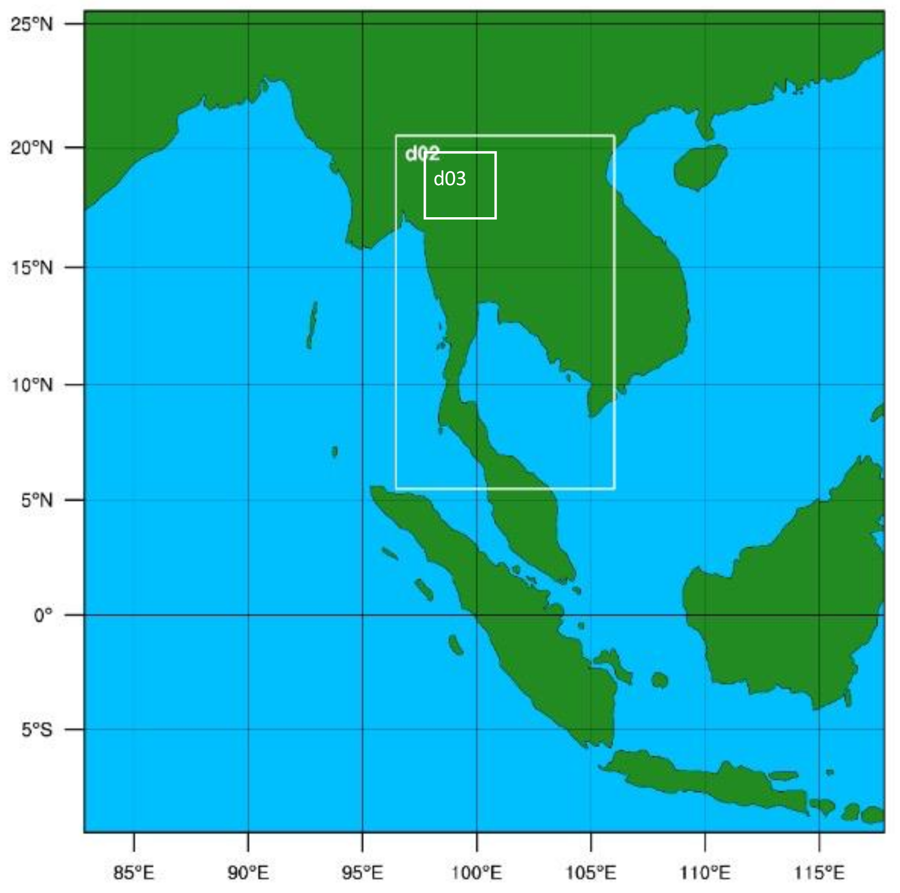
2.1. General Description and Set Up

We used the NRCM-Chem modeling system to simulate both time periods, including 1990–1999 and 2020–2029, with a single climate scenario based on the Representative Concentration Pathway (RCP)8.5. The model uses the CCSM version 4 as the meteorological initial and boundary conditions [29]. The model was coupled with the Price Weller Pinkel (PWP) model, which is an oceanic bulk mixing-layer model that consolidates the convection adjustment and shear instability of the mixing layer. It has now been developed for vertical mixing in the Hybrid Coordinate Ocean Model (HYCOM). The Runge–Kutta integration method [30] integrates several meteorological factors, i.e., wind, temperature, water vapor, and cloud hydrometeors. Additionally, the feedback and evolution of atmospheric aerosols on both short- and long-wave radiation were calculated in the model via the Rapid Radiative Transfer Model (RRTMG) radiation schemes [31]. Simultaneously, the model includes the feedback effects of aerosols on meteorological processes, such as the effects of aerosols on clouds and precipitation, which are computed by the Thompson scheme [32]. The Grell-3 scheme was responsible for subgrid-scale convection in the simulation. The land and atmospheric interactions were calculated via the Noah Land Surface Model [33]. For accurate large-scale meteorology, grid nudging [34] was applied in the outer domain for all vertical levels of the model, with nudging coefficients of 0.0003 s⁻¹ for all variables, including the horizontal wind, temperature, and water vapor every 6 h. An online biogenic emission calculation is performed with the Model of Emissions of Gases and Aerosols from Nature (MEGAN) version 2.04 [35]. In the NRCM-Chem simulations, gas-phase chemistry is represented by the MOZART chemistry mechanism [36] and aerosols by the MOSAIC representation [37]. A kinetic pre-processor and Rosenbrock solver [38] were applied to predict chemical concentrations from the gas-phase mechanism. The photolysis rates were computed using fast-TUV [39], which modifies the photolysis rates based on the presence of aerosols and clouds in each model grid cell. Dry deposition of gases and aerosols followed the Wesely [40] resistance method. Wet deposition of soluble gases was calculated using the method described by Neu and Prather [41]. The chemical variables from the Community Atmospheric Model with Chemistry (CAM-Chem), which is part of CCSM4, are used as chemical initial and boundary conditions for NRCM-Chem. CAM-Chem is a coupled chemistry-climate model that incorporates the Model for Ozone and Related Chemical Tracers (MOZART) chemical mechanism. CAM-Chem results from the Representative Concentration Pathway (RCP)8.5 scenario are implemented in our study.

However, because the simulation in regional climate and chemistry required a lot of computer resources for calculation and storage, especially when downscaled to a finer grid spacing (1 km), we only performed only one single case (the future change in climate and emissions). Furthermore, due to storage constraints, we restricted the model output by selecting some variables such as PM_2.5, precipitation, temperature, and relative humidity, resulting in the absence of some essential PM_2.5 chemical components such as ASOA, SO₄^2−, NH₄⁺, or NO₃⁻ that would be valuable in the analysis.

In this study, we used three domains that cover most of Southeast Asia and some parts of China. The first domain has 60-km grid spacing, the second domain in Thailand has 10-km grid spacing, and the finest domain has 1-km grid spacing that covers the northern peninsular Southeast Asia as shown in Figure 1. The vertical level was set to 53 levels from the surface up to 10 hPa near the tropopause. A one-way nesting technique was applied for forced initial and boundary conditions from the outer domain to the inner domain. The model has been run for two cases: (1) a present-day simulation (1990–1999) and (2) a future simulation (2020–2029). To examine the model’s predictive ability, the present-day model results from the inner domain were compared with several observation datasets, including the APHRODITE, the GPCP, the MERRA products, and ground-based measurements from the Thai Meteorological Department (TMD) and Pollution Control Department (PCD) in Thailand.

2.2. Emission

Emission data from the "Representative Concentration Pathways" (RCPs) databased of both anthropogenic and biomass burning inventories are used in the simulations. For the historical anthropogenic and biomass burning emissions, these are based on gridded emissions of reactive gases and aerosols for use in chemistry model simulations needed by climate models for the Climate Model Intercomparison Program 5 (CMIP5) in support of the Intergovernmental Panel on Climate Change (IPCC) Fifth Assessment report (AR5) [42]. There are 10 major chemical species, CH₄, CO, NO_x, NMVOC, CO₂, SO₂, BC and OC, with a spatial resolution of 0.5° × 0.5° (https://tntcat.iiasa.ac.at/RcpDb/dsd?Action=htmlpage&page=welcome, accessed on 10 February 2021). Anthropogenic emissions of reactive gases in 2000 are defined in terms of a variety of global and regional inventories. The historical emission in the simulation during year 1990 and1999 is computed in RETRO only. The emission inventory is well within the range of published estimates at the regional and global scales. While future emissions are based on RCP8.5 [43,44]. The RCP8.5 radiative forcing scenario generally developed by the MESSAGE modeling team and the International Institute for Applies Systems Analysis (IIASA) Integrated Assessment Framework in Austria. The RCP8.5 scenario is characterized by increasing greenhouse gas emissions over time representative for scenarios in the literature leading to high greenhouse gas concentration levels.

For the preparation of emissions for use with the model simulation, the mass-conserving method which does a better job of preserving integrals of the data, such as flux, between the source and target grids were used for mapping emissions to a given model grid. The key method of this method is the transition of data from one to another while maintaining the regional and local integrations, and this has many grids to another while maintaining the regional and local integrations and has many promising applications in atmospheric science [45].

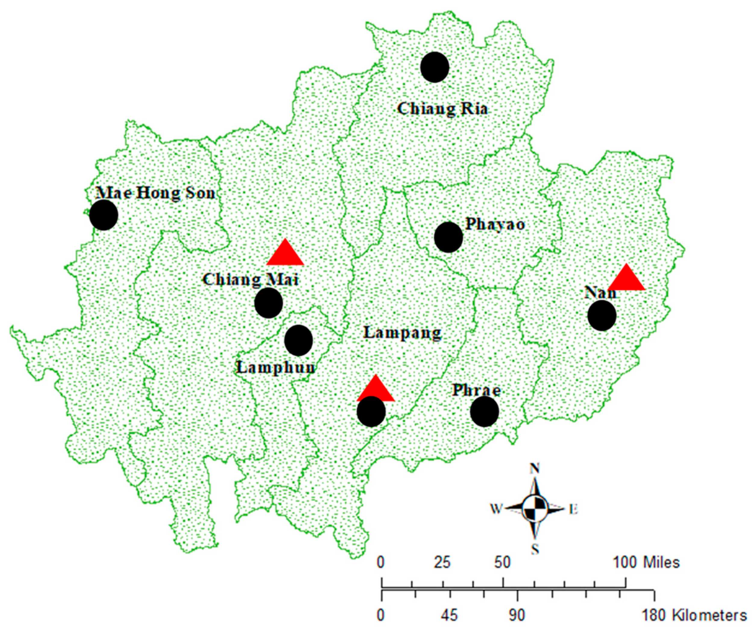
2.3. Observation Data

Ground-based measurements from the Thai Meteorological Department (TMD) were used to estimate PM_2.5 concentrations and evaluate models from 1990 to 1999, and the Pollution Control Department (PCD) was used to validate model performance in 2020. The location of station sites was shown in Figure 2. The site locations of the TMD ground-monitoring stations are located in the Thai Meteorological Department office, which is mostly in urban areas in each province. While the three ground-monitoring stations from PCD in urban areas selected as case studies: the Municipal Office in Nan, the Provincial Government Center in Chiang Mai, and the Meteorological Station in Lampang.

The general information of the quality control of climatology data was following the guidelines on the quality control of surface climatology data as follows: (1) data are coded by following a well-defined set of rules. These same rules can be incorporated into a computer program for checking the data. (2) Within one observation, the parameters are somewhat interrelated, and a simple check makes sure that the observation is consistent within itself. (3) The certain parameters are constrained within absolute limits, i.e., wind speed, and precipitation. (4) The extreme value will be queried and checked fairly soon after it occurs. (5) All the data are checked to see if they are within acceptable limits that is based on a simple method for detecting unrealistic values is to first rank the data then trim off the upper and lower 25%. From the remaining central 50% we determine the mean and the standard deviation from the half range (Abbott, 1986).

The Asian Precipitation—Highly Resolved Observational Data Integration Towards Evaluation of Water Resources (APHRODITE) project combines many datasets, including the Global Telecommunication System (GTS) precompiled dataset and individual collections. The GTS contains two datasets: the Global Summary of the Day (GSOD) and the Global Historical Climatology Network (GHCN) (GHCN). Furthermore, data from the Global Energy and Water Cycle Experiment (GEWEX), the Asian Monsoon Experiment (GAME), and the Association of Southeast Asian Nations (ASEAN) are included in the precompiled dataset. The APHRODITE project’s data came from national meteorological and hydrological services (NMHs) or individuals in Japan, China, Mongolia, Russia, Taiwan, and Nepal. The dataset, with a resolution of 0.5° × 0.5°, covers the Asian continent from 1973 to 2007 [46].

The Global Precipitation Climatology Project (GPCP) data, version 2, is a monthly precipitation dataset for the entire world. The data ranges from 1979 to the present, with a precision of 1° × 1°. The dataset was created by combining satellites from low-orbit satellite microwave data based on Special Sensor Microwave Imager (SSM/I) data from Defense Meteorological Satellite Program (DMSP, Virginia, United States) satellites, geosynchronous-orbit satellite infrared data from Special Sensor Microwave Imager (SSM/I) data from Defense Meteorological Satellite Program (DMSP, United States) satellites, and surface observation data from the Global Telecommunications Network (GTN) [47].

The Modern-Era Retrospective Analysis for Research and Applications, version 2 (MERRA-2) is a reanalysis of atmospheric data generated by NASA’s Global Modeling and Assimilation Office (GMAO) with a resolution of 0.5° × 0.6°. Several aspects, including as stratospheric representation and cryosphere processes, have been updated from limitations in the previous version of MERRA. MEERA-2’s water cycle has also been improved. This dataset has mostly incorporated Integrated Earth System Analysis (IESA) into the future dataset. The data can be accessed via the NASA Goddard Earth Sciences Data Information Services Center (GES DISC) [48].

2.4. Estimation of PM_2.5 for Model Evaluation

Because there were no PM_2.5 observations in Thailand between 1990 and 1999, this study used alternate methodologies to estimate PM_2.5 concentrations. The linear multivariate linear regression model that includes meteorological parameters, i.e., Aerosol Optical Depth (AOD), temperature, relative humidity, and wind speed, was conducted for estimating PM_2.5 concentrations over northern Thailand during 1990 to 1999. The equation was given as follows [49] in Equation (1):

$${\mathrm{PM}}_{2.5}=\left(\mathsf{\alpha }+{\mathsf{\epsilon }}_1\right)+\left({\mathsf{\beta }}_1+{\mathsf{\epsilon }}_1\right)\times \mathrm{AOD}+\left({\mathsf{\beta }}_2+{\mathsf{\epsilon }}_3\right)\times \mathrm{Temp}+\left({\mathsf{\beta }}_3+{\mathsf{\epsilon }}_4\right)\times \mathrm{RH}+\left({\mathsf{\beta }}_4+{\mathsf{\epsilon }}_5\right)\times \mathrm{WSPD}$$

(1)

where PM_2.5 is its mass concentration at ground level (μg/m³), AOD is derived from MODIS (dimensionless), Temp is temperature (°C), RH is relative humidity (%), WSPD is wind velocity (m/s), β₁, β₂, … β₈ are the slopes corresponding to the respective variables, and (α + ε₁) is the intercept.

To estimate PM_2.5 concentration during 1990–1999, here, we used the data including temperature, relative humidity, and wind speed from TMD at eight ground monitoring stations in northern Thailand, including Nan, Chiang Mai, Lampang, Lamphun, Chiang Rai, Phayao, Phrae, and Mae Hong Son (Figure 2).

The temperature, humidity, and wind speed were measured as the following the guide and methods of the World Meteorological Organization (WMO) (https://library.wmo.int/doc_num.php?explnum_id=10616, 10 February 2021). Thermometer readings of air temperature were collected on a continuous basis at various time intervals. The data obtained were derived as the mean of a collection of 1 min measurements. With a sensor time constant of 20 s, the operational measurement uncertainty of temperature was in the range of (−80)–(+60) °C. While a hygrometer is used to measure humidity, it has a performance range of (5)–(100)% and an achievable observing uncertainty of 3–5 % for relative humidity. A wind vane with a cup or propeller anemometer are commonly used to measure surface wind. The output averaging time is 2 or 10 min, with an uncertainty of 0–360° and a sensor time constant of 1 s. Wind speed estimates are based on the effect of the wind on movable objects, with an uncertainty of 0–75 m/s and a sensor time constant of 2–5 m of distance constant.

In addition, AOD product data during 1990–1999 from Multi-angle Imaging SpectroRadiometer (MISR) Level 2 Aerosol Retrieval were also retrieved. This data set is based on a MERRA-2 monthly mean with descriptive short name “instM_2d_gas_Nx” and short name “M2IMNXGAS”. The data product is available through Giovanni at 550 nm from the Moderate Resolution Imaging Spectroradiometer (MODIS); at 865 and 869 nm from the Sea-viewing Wide Field-of-view Sensor (SeaWiFS); at 443, 555, 670, and 865 nm from the Multi-angle Imaging SpectroRadiometer (MISR); and at several wavelengths between 342 and 500 nm from Aura’s Ozone Measuring Instrument (OMI). OMI also provides Aerosol Absorption Optical Depth for near-UV wavelengths [50].

2.5. Statistical Used

In addition, the model was evaluated for reliability using statistical analysis including R-squared, mean bias, standard deviation of residuals, and index of agreement. The mean bias is calculated following Equation (2):

$$\mathit{M}\mathit{e}\mathit{a}\mathit{n} \mathit{B}\mathit{i}\mathit{a}\mathit{s}=\overline{\mathit{M}}-\overline{\mathit{O}}$$

(2)

where $\overline{\mathit{M}}$ is the average of the model data, and $\overline{\mathit{O}}$ is the average of the observed data. The standard deviation of residuals (SDR) is calculated following Equation (3):

$$\mathit{S}\mathit{D}\mathit{R}=\sqrt{\frac{\sum {[\left({\mathit{x}}_{\mathit{O}}-{\mathit{X}}_{\mathit{M}}\right)-\left(\overline{{\mathit{X}}_{\mathit{O}}}-\overline{{\mathit{X}}_{\mathit{M}}}\right)]}^2}{\mathit{n}}}$$

(3)

where ${\mathit{X}}_{\mathit{O}}$ is the observed data, ${\mathit{X}}_{\mathit{M}}$ is the model data, $\overline{{\mathit{X}}_{\mathit{O}}}$ is the mean of the observed data, $\overline{{\mathit{X}}_{\mathit{M}\mathit{O}}}$ is the mean of the model data, and n is the number of values in the model and observed data.

The index of agreement (IOA) is calculated following Equation (4):

$$\mathrm{IOA}=1-\left[\frac{{\displaystyle \sum _1^n{\left(O-M\right)}^2}}{{\displaystyle \sum _1^n{\left(\left|M-\overline{O}\right|+\left|O-\overline{O}\right|\right)}^2}}\right]$$

(4)

where O is the observed data, M is the model data, $\overline{O}$ is the mean of the observed data, and n is the number of values in the model and observed data.

The fraction error is calculated following Equation (5):

$$\mathrm{Fractional} \mathrm{Error}=\frac{1}{n}\left(\frac{{\displaystyle \sum _1^n\left|M-O\right|}}{{\displaystyle \sum _1^n\left(\frac{\left(M+O\right)}{2}\right)}}\right)$$

where M is the model data and O is the observed data.

While the correlation coefficients of Pearson, Spearman, and Kendall as well as Maximal Information Coefficient (MIC) were used for the analysis of the driver PM_2.5 in the future. The equation of the Pearson and Maximal Information Coefficients (MIC) follow Equations (5) and (6) [51,52]:

$$\mathit{r}=\frac{\sum \left({\mathit{x}}_{\mathit{i}}-\overline{\mathit{x}}\right)\left({\mathit{y}}_{\mathit{i}}-\overline{\mathit{y}}\right)}{\sqrt{\sum {\left({\mathit{x}}_{\mathit{i}}-\overline{\mathit{x}}\right)}^2}\sum {\left({\mathit{y}}_{\mathit{i}}-\overline{\mathit{y}}\right)}^2}$$

(5)

where r is correlation coefficient;

${\mathit{x}}_{\mathit{i}}$ and ${\mathit{y}}_{\mathit{i}}$ are variable of any x and y;

$\overline{\mathit{x}} \mathrm{and} \overline{\mathit{y}}$ re averaged of any x and y;

$$\mathit{M}\mathit{I}\mathit{C} \left(\mathit{x},\mathit{y}\right)=\mathit{m}\mathit{a}\mathit{x}\left\{\frac{\mathit{I}\left(\mathit{x},\mathit{y}\right)}{\mathit{l}\mathit{o}{\mathit{g}}_2\mathit{m}\mathit{i}\mathit{n}\left\{{\mathit{n}}_{\mathit{x}},{\mathit{n}}_{\mathit{y}}\right\}}\right\}$$

(6)

where x, y are any variables, and I is the percent of a variable y that can be explained by a variable y.

3. Results and Discussion

This section begins with the model evaluation section to assess the model’s performance. For the 2 m-temperature and precipitation, the model results were compared to the observation data, while the modeled PM_2.5 was compared to both estimation techniques during 1990–1999 and ground-based measurements in 2020. Then, the difference between the PM_2.5’s precursors in the near-future (2020–2029) and the past (1990–1999) was revealed in Section 3.2. The difference in temperature, precipitation, and PM_2.5 between the near-future and the past was shown in Section 3.3. Lastly, the driver of PM_2.5 during 2020–2029 was analyzed using a statistical approach.

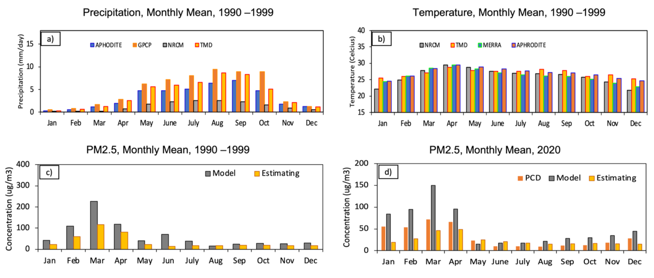
3.1. Model Evaluation

To examine the performance of the multivariate linear regression model, the estimation of PM2.5 was compared to the average of ground-based measurement data at three locations from the Pollution Control Department (PCD) in the year 2020, as shown in

Table 1. The statistical comparisons between model, observation, and estimation in northern Thailand.

Statistical Analysis	Temperature	Precipitation	PM2.5
			Obs. vs. Model (2020)	Obs. vs. Estimate (2020)	Estimate vs. Model (1990–1999)
IOA	0.76	0.63	0.80	0.77	0.79
Mean-Bias	−0.92	−2.68	21.9	−7.3	28.75
Fractional Error	8.81	0.061	0.043	0.039	0.048
SDR	1.87	2.54	30.2	16.7	60.00

. The multivariate linear regression model shows a good result for estimating overall PM_2.5 concentrations as indicated by the IOA value of 0.77, and the mean bias was −7.3 µg/m³, the fractional error was 0.039, and the SDR was 16.7. Moreover, as shown in Table 1, the statistical calculations between the model data and the observed data from PCD are averaged throughout the year 2020 from three PCD station locations. This is demonstrated by IOA values of 0.80, which indicates a good ability to capture PM_2.5 patterns. The modeled PM_2.5 in the year 2020 was overestimated when compared to the PCD data, with a mean bias error of 21.9 µg/m³ and fractional error of 0.043.

The monthly mean 2m-temperature and precipitation from the model’s finer domain averaged from 1990 to 1999 are compared to ground-based observations from TMD, APHRODITE, MERRA, and GPCP based on eight TMD station locations in northern Thailand (Figure 3a,b). The NRCM accurately predicts the monthly and daily temperature and precipitation patterns. The modeled temperature has a cold bias in January to February and November to December, while the total amount of precipitation is anticipated to be lower for the entire year. Figure 3b clearly demonstrates a cold bias and an underestimation of temperature and precipitation. Temperatures are colder in the dry season (November to April), notably from November to February, by 1–2 °C. In general, the modeled precipitation agrees fairly well with the TMD dataset. The amount of precipitation has decreased by 1–5 mm/day. The monthly mean PM_2.5 from the model’s finer domain averaged from 1990 to 1999 is compared to the estimation from ground-based observations from TMD in northern Thailand (Figure 3c). The model accurately represents the monthly PM_2.5 pattern. The modeled PM_2.5 concentration was found to be significantly overestimated from February and March, and underestimated from August to December. The statistical comparisons between model data and observed TMD data are averaged during the period 1990–1999 from eight TMD station locations, as shown in Table 1. The model is highly capable of reproducing both temperature and precipitation, as evidenced by IOA (0.76 for temperature and 0.63 for precipitation). The modeled temperature and precipitation are underestimated in comparison to data, with a mean bias of (−0.92) °C and (−2.68) mm, respectively. The standard deviations of the model’s residuals are 1.87 and 2.54 for temperature and precipitation, respectively. As indicated in

Table 2. The percentage difference in annual, dry season and wet season of total emission of BC, CH₄, CO, NH₃, NO_x, and SO₂ between the time periods of 1990–1999 and 2020–2029.

Chemical Species	Annual	Dry Season	Wet Season
	% Diff.	% Diff.	% Diff.
BC	−5.12	11.86	−0.13
CH4	−1.86	11.74	−4.32
CO	−1.92	11.21	−4.39
NH3	5.22	9.60	−11.90
NOx	−3.47	12.00	−2.87
SO2	3.44	9.75	−10.52

, the statistical calculations between the model data and the estimation are averaged during the period 1990–1999 from three TMD station locations. The model has a high capacity for capturing PM_2.5, as indicated by IOA values of 0.79. The modeled PM_2.5 concentrations are higher than those estimated, with a mean bias of 28.75 µg/m³. For PM_2.5, the standard deviation of the residuals from the model and estimation was 60, while the fractional error was 0.048.

Although, the high-resolution model provides more spatial information compared to the coarse resolution, the regional climate set up in this study was similar to a previous study in Amnuaylojaroen and Chanvichit, 2019 so, the underestimation for precipitation and cold bias for temperature was also found. There are various possibilities that resulted in simulation errors. For example, the model employs grid-nudging to maintain the large-scale meteorology from the Global climate model, therefore the error from initial and boundary conditions should be addressed. To begin, describing the Intertropical Convergence Zone (ITCZ) is complicated. Low precipitation and sea surface temperatures are found across the Indian Ocean in the CCSM4, as mentioned in Gent et al. [29], Danabasoglu et al. [53], Yuan et al. [54], and Yang et al. [55] and have a substantial influence on the Asian monsoon. Another possibility, as noted in Trenberth [56], Koster et al. [57], and Hong et al. [58], is the absence of a soil moisture routine in the model calculation which is dominated by local evaporation from the moisture recycling process in the tropical region.

The overestimation of the PM_2.5 concentrations, particularly, in March and April also similar to an early study by Nguyen et al. [59] who examined the simulated PM_2.5 and O₃ in Southeast Asia using the Weather Research and Forecasting (WRF) model and the Community Multiscale Air Quality (CMAQ) model. They suggest that there were several factors that could affect the model performance such as emission input data accuracy and spatial resolution. The observations were point-based at individual observation sites and might be affected by local emissions nearby, whereas the modeled concentrations were grid average values. However, to clearly address these discrepancies between simulations and observations, further studies on the emissions, mechanisms, and meteorology in the region are required. Both the observations and simulations mostly showed high PM_2.5 concentrations during the dry season compared to those during the wet season. Furthermore, Georgiou et al. [60] postulated that the MOSAIC aerosol process overestimates PM_2.5 concentrations due to a larger dust component. MOSAIC, for example, slightly underestimates nitrate aerosols. These changes are due to the different handling of gas-to-particle partitioning from nitric acid to ammonium nitrate as a function of humidity [61], which MOSAIC employs using the Zaveri et al. [62] method that the diurnal cycle of relevant chemical component such as NO₃ and N₂O₅ are crucial during nighttime. Furthermore, the MOSAIC mechanism drastically underestimates elemental carbon (EC) concentrations due to the lack of anthropogenic emissions in this mechanism, which were attributed to chemical processes that act as H₂SO₄ sources/sink. The discrepancy from biomass burning emission for simulation of PM_2.5 was revealed by Pimonsree et al. [63], who conducted the coupled WRF-CMAQ modeling system in northern Thailand. Their results shows that the improved biomass burning emission could improve IOA from 0.24 to 0.55.

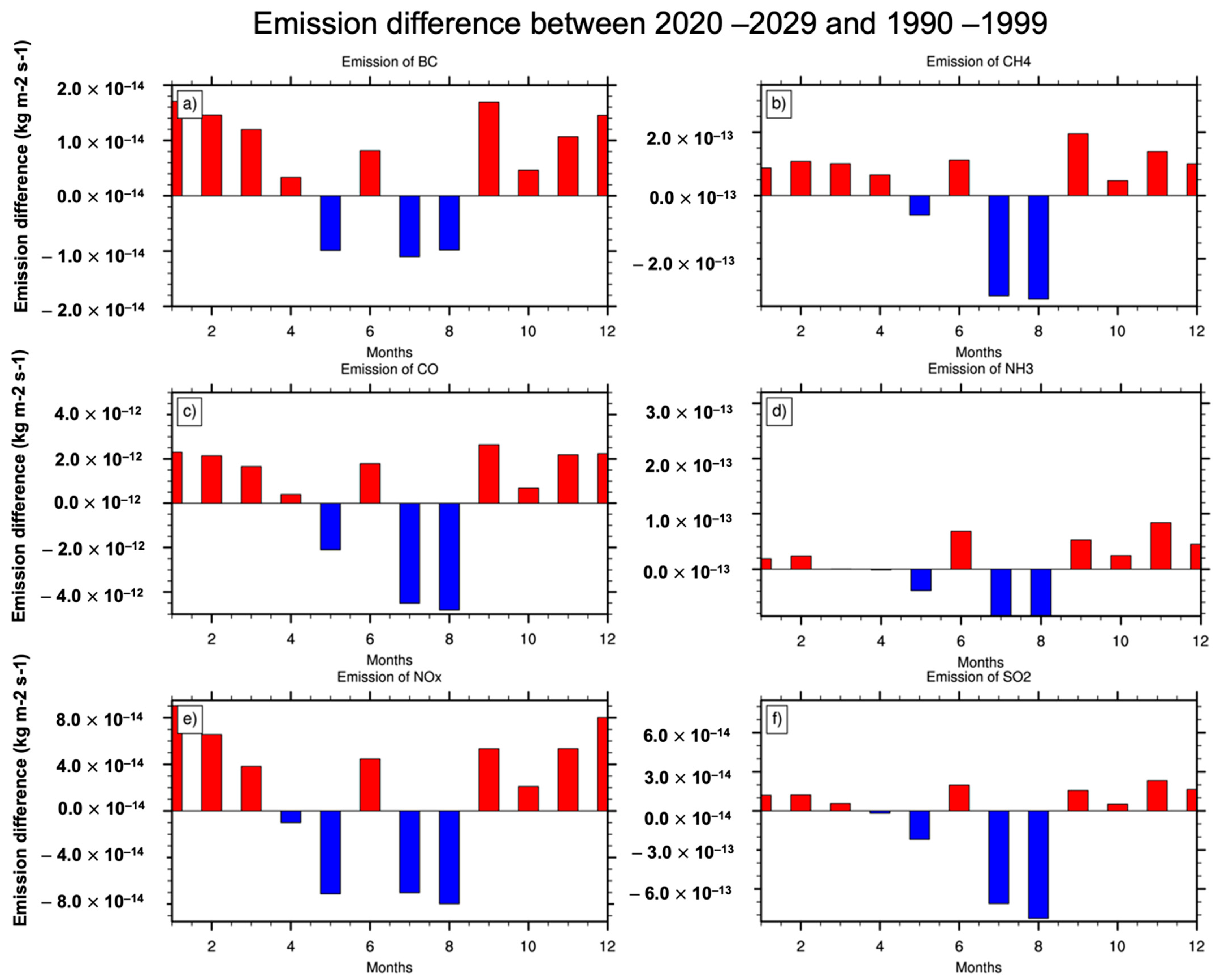
3.2. Emission of PM_2.5′s Precursors during 2020–2029

PM_2.5 particles are complex because they can be made up of numerous types of chemicals and particles. It comes from a variety of sources, making it a very complex type of pollution. There were many of the major components of the precursors of PM_2.5 that form secondary PM_2.5 through the reactive process, including black carbon, nitrate, sulfate, ammonia, and organic carbon. Black carbon, which is essentially soot, and soil are the main sources of primary PM_2.5 [64]. The other components that are listed as secondary components of PM_2.5 are not emitted from sources directly, but contribute to PM_2.5 through chemical reaction, coagulation, and other mechanisms. Secondarily formed PM_2.5 particles typically are derived from the formation of either ammonium sulfate or ammonium nitrate, through the chemical reaction of ammonia and SO₂ (in the presence of water) or ammonia and NO_x. In addition, secondary particles are developed via the chemical reaction of ozone and organic gases (organic carbon) in the atmosphere.

Here, we focused on the emissions of BC, CH₄, CO, NH₃, NO_x, and SO₂ over northern Thailand. The emissions were derived from the combination between anthropogenic and biomass burning emissions for the years 1990–1999 and 2020–2029. Figure 4 shows the monthly emission difference of BC, CH₄, CO, NH₃, NO_x, and SO₂ between year 2020–2029 and 1990–1999 over northern Thailand. All six chemical species tend to increase in the dry season (November to April) and decrease in the wet season (May to October). Table 2 presents the past emissions, the future anthropogenic emissions, and the percentages of emission changes in the future period compared with the past period of major PM_2.5 precursors. In general, there was not much difference in emissions among the whole year, while the emissions during the dry season tend to increase. In contrast, the wet season tend to decrease all of six chemical species considered as PM_2.5 precursors. The seasonal difference in emissions in this region is likely dominated by biomass burning. As reported in previous studies, fire from biomass burning is an important source that releases several chemical species such as NO_x, CO, and VOCs in the dry season, especially during the peak of biomass burning, which is typically in February and March [65,66]. In the present period, among six chemical species, emissions of CO were higher than other chemical species. In the future period, all six chemical species, BC, CH₄, CO, NH₃, NO_x, and SO₂, show increasing trends in their emissions during the dry season and decreasing trends during the wet season. Over six chemical species, emissions in the future period were estimated to increase by 11.86 % for BC, 11.74% for CH₄, 11.21% for CO, 9.60% for NH₃, 12% for NO, and 9.75 % for SO₂ during the dry season, while decreasing in the wet season by −0.13 for BC, −4.32 for CH₄, −4.39 for CO, −11.90 for NH₃, −2.87 for NO_x, and −10.52 for SO₂.

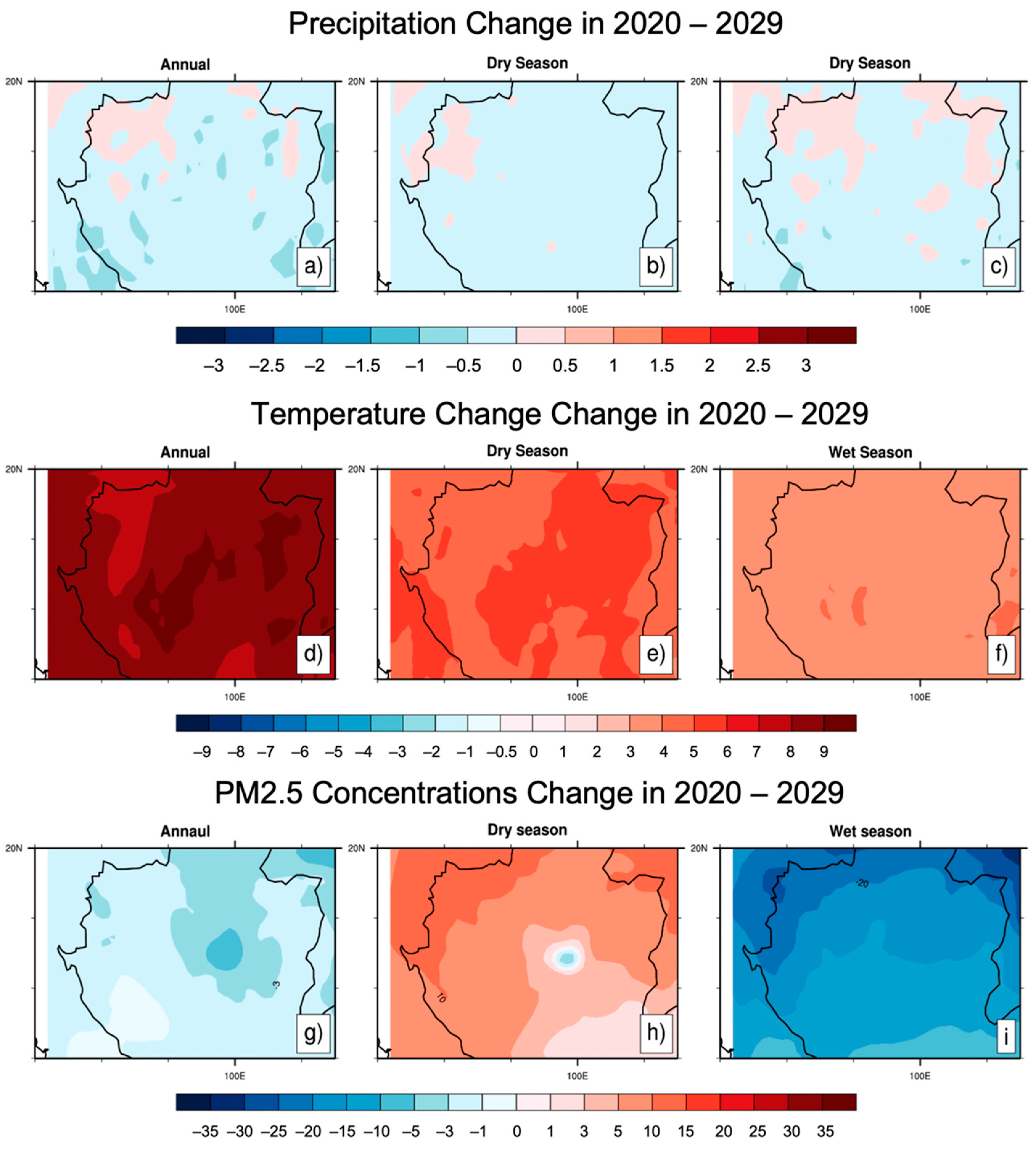
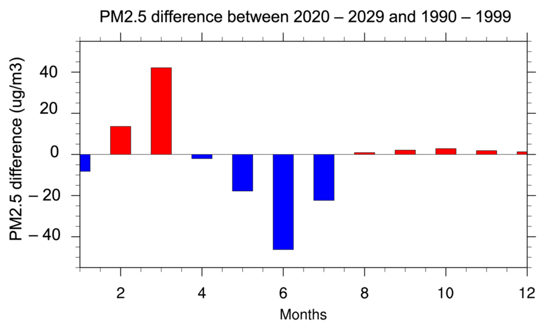
3.3. Projection of Precipitation, Temperature, and PM_2.5

Figure 5a–f display changes in seasonal spatial precipitation and 2m-temperature over northern Thailand. Future precipitation generally tends to decrease in ranges of (0.5)–(−1) mm/day throughout northern Thailand during the dry season, wet season, and for the whole year. In contrast, the 2m-temperature tends to increase throughout northern Thailand in ranges of (+1)–(+9) °C. There is much more change in temperature for the whole year compared with the dry season and the wet season over all of the study area. The combined changes in climatic factors and emissions in the previous section will likely affect air quality in northern Thailand in the future. The projected change in PM_2.5 concentrations between the years 2020–2029 and 1990–1999 over northern Thailand are shown in Figure 5g–h. In general, the annual PM_2.5 concentration tend to decrease across the region in the future. Between the dry season and the wet season, there is a difference in the contribution of emission concentration, especially from biomass burning emissions [67,68]. However, the projected emission change mostly brings about increases in PM_2.5 concentration on average and in the range of (+1) to (+35) μg/m³ during the dry season (November to April), and decreases on average and in range of (−3) to (−30) μg/m³ during the wet season (May to October). The maximum increase in PM_2.5 concentrations found in February and March were 10 ug/m³ and 40 ug/m³, respectively (Figure 6). For March, the PM_2.5 extremely increased compared to other months by more than 40 ug/m³. While the strongly decreasing PM_2.5 was found in June by more than (−40) ug/m³. In addition, the difference is induced by the meteorological condition difference between these two seasons. During the wet season, the PM_2.5 concentration is slightly lower than that during the dry season in terms of the magnitude because precipitation during the wet season is higher than that during the dry season [26].

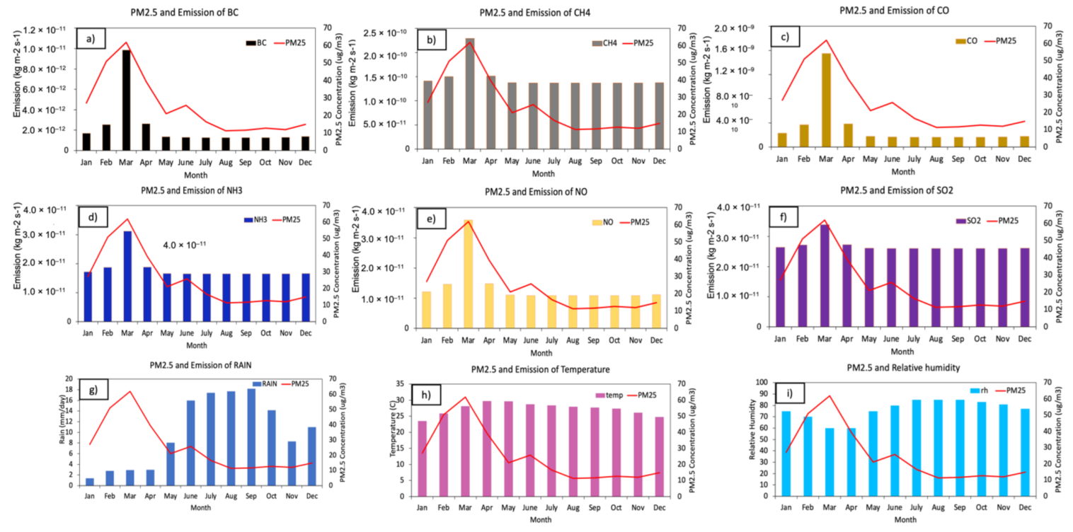
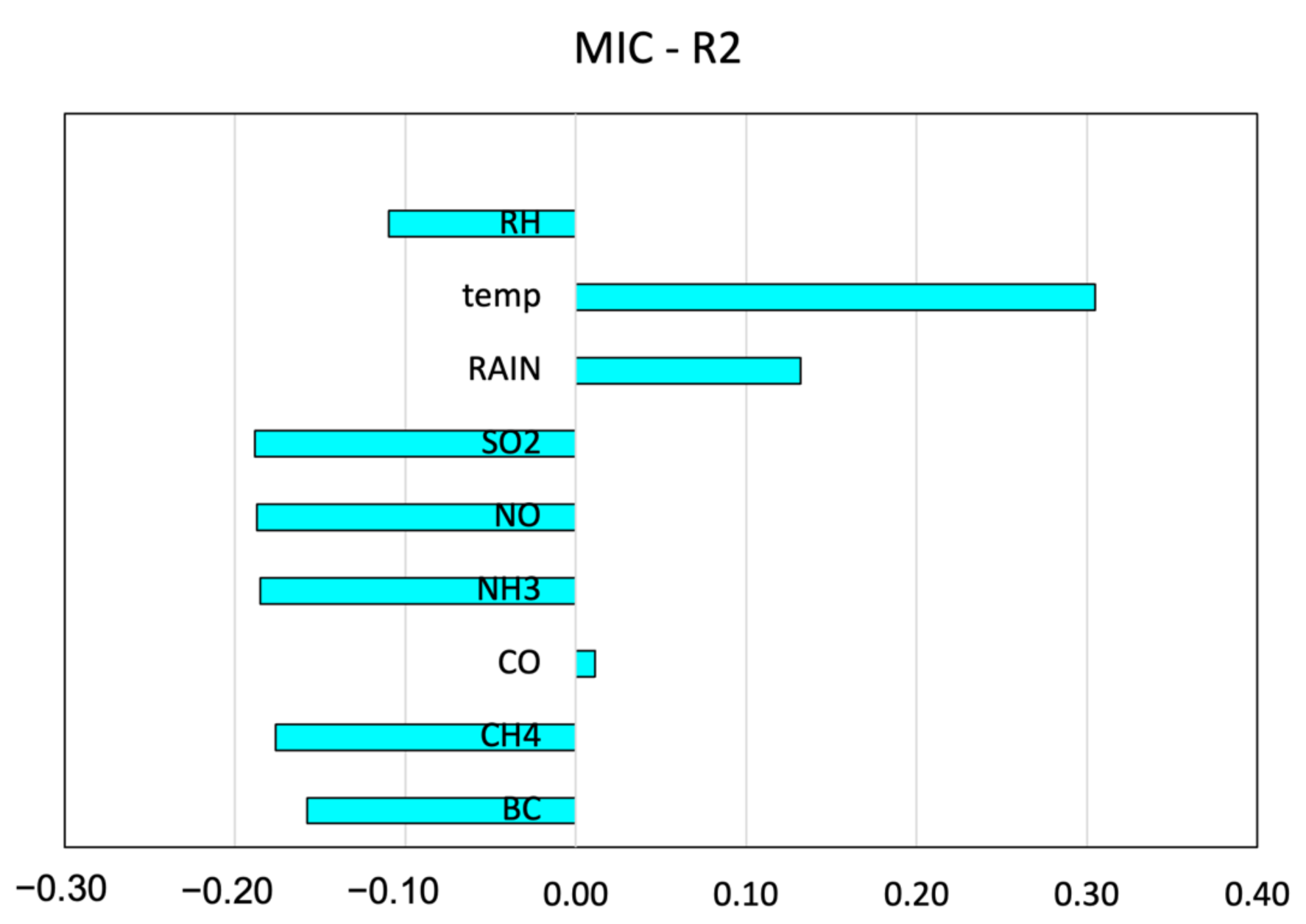
3.4. The Drivers of PM_2.5 during 2020–2029 over Northern Thailand

The plot of correlation of the averaged future PM_2.5 concentration and its chemical components BC, CH₄, CO, NH₃, NO, and SO₂ and meteorological factors precipitation, temperature, and relative humidity over northern Thailand is displayed in Figure 7. In addition, the relationships between the concentrations of PM_2.5 chemical components including BC, CH₄, CO, NH₃, NO, and SO₂ and some meteorological factors including precipitation, temperature, and relative humidity were examined using Pearson correlation coefficient, Kendall correlation coefficient, Spearman’s rank correlation, and Maximal Information Coefficient. A non-parametric correlation matrix was constructed separately for the averaged data during 2020–2029 as listed in

Table 3. Correlation between PM_2.5 and emission data and climate parameter during 2020–2029.

	PM2.5
	Pearson	MIC
BC	0.79	0.46
CH4	0.80	0.46
CO	0.80	0.65
NH3	0.80	0.46
NO	0.80	0.46
SO2	0.80	0.46
Precipitation	−0.72	0.65
temp	0.08	0.31
RH	−0.88	0.65

It can be seen that all of the chemical components’ emissions are related to PM_2.5 concentrations. It has a gradual increase steadily from January to March and is the highest emission value in March in all chemical species, especially carbon monoxide (CO) emissions by 1.5 × 10⁻⁹. The precipitation was found to be relevant as well. It will find the amount of rain that falls less than other months. The average precipitation was 1–3 mm/day during the months of January to March.

The correlation between PM_2.5 and emission data and climate parameter during 2020–2029 is shown in Table 3. PM_2.5 concentrations showed a strong positive correlation with all of chemical species, 0.79–0.80 for Pearson coefficient, and showed a moderate positive correlation with all of chemical species for MIC values in the ranges of (+0.46)–(+0.65). Meanwhile, some meteorological parameters such as precipitation and relative humidity showed a strong negative correlation with the PM_2.5 concentration by (−0.72) and (−0.88) for the Pearson coefficient. Furthermore, the strong positive correlation was found for MIC value by 0.31 for temperature and 0.65 for both precipitation and relative humidity. When considering the difference of the coefficient MIC − R² ≈ 0 (Figure 8), that is, the closer the difference is to 0 indicates that the two variables are linearly correlated, but if the relationship between the two variables is non-linear, the difference between the MIC value and the R-squared value will be higher. In addition, CO emissions likely tend to contribute to PM_2.5 concentrations in northern Thailand in the future, indicated by the high correlation and lower difference of the coefficient MIC − R². Even though sulfate (SO₄²⁻) and nitrate (NO₃⁻) are widely recognized as the two most sensitive factors contributing to PM_2.5 [69], they are produced by the oxidation of SO₂, NO_x, and volatile organic molecules (VOCs). SO₄²⁻ can be produced by oxidizing SO₂ in the gas phase with OH or by oxidizing SO₂ in water with dissolved H₂O₂ or O₂ [70]. During the day, nitrate synthesis is dominated by NO₂ with hydroxyl radical (OH) followed by condensation, whereas, at night, nitrate radical (NO₃) or dinitrogen pentoxide (N₂O₅) heterogeneous processes predominate [71]. However, carbon monoxide (CO) has an indirect effect. When it reacts with the hydroxyl radical, the hydrogen atom immediately interacts with O₂ to generate the hydroperoxyl radical HO₂. The most important atmospheric reaction that HO₂ undertakes when NO is present is that with NO [14].

However, there were some shortcomings in this work. As suggested by Nguyen et al., 2019, the emission is very sensitive in Southeast Asia, so additional cases, such as future climate change with constant emissions, future climate change with different types of emissions including anthropogenic, biomass burning, and biogenic emissions should be conducted for the future work. This study simulates both climatic and chemical factors over a 10-year period, which is insufficient to construct an average climatology and thus eliminates interdecadal variability. Given the actual restrictions of available resources, this was a necessary constraint, and an improvement over previous work that concentrated exclusively on one-year durations (e.g., Adachi et al., 2014; Yang et al., 2016). We believe the findings are still useful since they demonstrate how climate and emissions changes can affect the PM_2.5 concentration. Future research should look at a longer time span, such as 30 years, to capture more variability in the atmosphere.

4. Conclusions

In this study, we evaluate the influence of climate and emission changes on PM_2.5 concentrations on the northern peninsula of Southeast Asia, which is located in the northern part of Thailand. The Nested Regional Climate with Chemistry Model (NRCM-Chem) was performed from 1990 to 1999 as the past and 2020 to 2029 as the near-future under RCP8.5. In the simulations, the emission data from the "Representative Concentration Pathways" (RCPs) database of both anthropogenic and biomass burning inventories are employed. The CCSM version 4 is utilized as the meteorological initial and boundary conditions, while the chemical variables from the Community Atmospheric Model with Chemistry (CAM-Chem) are used as the chemical initial and boundary conditions for NRCM-Chem.

The monthly mean 2 m-temperature and precipitation from the model’s finer domain averaged from 1990 to 1999 are compared to ground-based measurements from TMD, APHRODITE, MERRA, and GPCP based on 8 TMD station locations in northern Thailand. While the PM_2.5 comparison was used both the estimation from the linear multivariate linear regression model, which includes meteorological parameters such as Aerosol Optical Depth (AOD), temperature, relative humidity, and wind speed, was used to estimate PM2.5 concentrations over northern Thailand from 1990 to 1999, and the ground-based measurement data from three PCD station location in northern Thailand in the year 2020. As demonstrated by IOA, the model is very capable of recreating temperature, precipitation and PM_2.5 concentration (0.76 for temperature, 0.63 for precipitation, and 0.79 and 0.80 for PM_2.5 concentration). The modeled temperature and precipitation are both underestimated when compared to the observation data, with a mean bias of (−0.92) °C and (−2.68) mm, respectively. While a modeled PM_2.5 values are overestimated, with a mean bias of 28.75 µg/m³ and 21.9 µg /m³, when compared to the estimation technique and PCD data.

Climate change increasing temperatures and decreasing precipitation will most certainly have an impact on northern Thailand’s air quality. As a result of changes in the climatic parameters and emissions of PM_2.5′s precursors, PM_2.5 concentrations increase across the region in the range of (+1) to (+35) µg/m³ during the dry season (November to April) and decrease on average in the range of (−3) to (+3) µg/m³ during the wet season (May to October) and in the range of (−1) to (−10) µg/m³ for the entire year. In particular, PM_2.5 levels for a complete domain increased by more than 40 µg/m³ in March when compared to other months.

References

1. Jacob, D.J.; Winner, D.A. Effect of climate change on air quality. Atmos. Environ. 2009, 43, 51–63. [Google Scholar] [CrossRef] [Green Version]
2. Dawson, J.P.; Racherla, P.N.; Lynn, B.H.; Adams, P.J.; Pandis, S.N. Impacts of climate change on regional and urban air quality in the eastern United States: Role of meteorology. J. Geophys. Res. Atmos. 2009, 11. [Google Scholar] [CrossRef] [Green Version]
3. Kleeman, M.J. A preliminary assessment of the sensitivity of air quality in California to global change. Clim. Chang. 2008, 87, 273–292. [Google Scholar] [CrossRef]
4. Hedegaard, G.B.; Brandt, J.; Christensen, J.H.; Frohn, L.M.; Geels, C.; Hansen, K.M.; Stendel, M. Impacts of climate change on air pollution levels in the Northern Hemisphere with special focus on Europe and the Arctic. Atmos. Chem. Phys. 2008, 8, 3337–3367. [Google Scholar] [CrossRef] [Green Version]
5. Steiner, A.L.; Tonse, S.; Cohen, R.C.; Goldstein, A.H.; Harley, R.A. Influence of future climate and emissions on regional air quality in California. J. Geophys. Res. Atmos. 2006, 111. [Google Scholar] [CrossRef]
6. Yin, S.; Wang, X.; Zhang, X.; Guo, M.; Miura, M.; Xiao, Y. Influence of biomass burning on local air pollution in mainland Southeast Asia from 2001 to 2016. Environ. Pollut. 2019, 254, 112949. [Google Scholar] [CrossRef]
7. Lee, H.-H.; Iraqui, O.; Gu, Y.; Yim, S.H.-L.; Chulakadabba, A.; Tonks, A.Y.-M.; Yang, Z.; Wang, C. Impacts of air pollutants from fire and non-fire emissions on the regional air quality in Southeast Asia. Atmos. Chem. Phys. 2018, 18, 6141–6156. [Google Scholar] [CrossRef] [Green Version]
8. Lee, H.-H.; Iraqui, O.; Wang, C. The impact of future fuel consumption on regional air quality in Southeast Asia. Sci. Rep. 2019, 9, 2648. [Google Scholar] [CrossRef]
9. Colette, A.; Bessagnet, B.; Vautard, R.; Szopa, S.; Rao, S.; Schucht, S.; Klimont, Z.; Menut, L.; Clain, G.; Meleux, F. European atmosphere in 2050, a regional air quality and climate perspective under CMIP5 scenarios. Atmos. Chem. Phys. 2013, 13, 7451–7471. [Google Scholar] [CrossRef] [Green Version]
10. Zhang, Y.; Wang, K.; Jena, C. Impact of projected emission and climate changes on air quality in the US: From national to state level. Procedia Comput. Sci. 2017, 110, 167–173. [Google Scholar] [CrossRef]
11. Amann, M.; Klimont, Z.; Wagner, F. Regional and global emissions of air pollutants: Recent trends and future scenarios. Annu. Rev. Environ. Resour. 2013, 38, 31–55. [Google Scholar] [CrossRef]
12. Fiore, A.M.; Naik, V.; Leibensperger, E.M. Air quality and climate connections. J. Air Waste Manag. Assoc. 2015, 65, 645–685. [Google Scholar] [CrossRef]
13. Choi, D.H.; Kang, D.H. Infiltration of ambient PM2. 5 through building envelope in apartment housing units in Korea. Aerosol Air Qual. Res. 2017, 17, 598–607. [Google Scholar] [CrossRef] [Green Version]
14. Amnuaylojaroen, T.; Macatangay, R.C.; Khodmanee, S. Modeling the effect of VOCs from biomass burning emissions on ozone pollution in upper Southeast Asia. Heliyon 2019, 5, e02661. [Google Scholar] [CrossRef] [Green Version]
15. Lelieveld, J.; Barlas, C.; Giannadaki, D.; Pozzer, A. Model calculated global, regional and megacity premature mortality due to air pollution. Atmos. Chem. Phys. 2013, 13, 7023–7037. [Google Scholar] [CrossRef] [Green Version]
16. Vichit-Vadakan, N.; Ostro, B.D.; Chestnut, L.G.; Mills, D.M.; Aekplakorn, W.; Wangwongwatana, S.; Panich, N. Air pollution and respiratory symptoms: Results from three panel studies in Bangkok, Thailand. Environ. Health Perspect. 2001, 109, 381–387. [Google Scholar]
17. Tsai, F.C.; Smith, K.R.; Vichit-Vadakan, N.; D OSTRO, B.; Chestnut, L.G.; Kungskulniti, N. Indoor/outdoor PM 10 and PM 2.5 in Bangkok, Thailand. J. Expo. Sci. Environ. Epidemiol. 2000, 10, 15–26. [Google Scholar] [CrossRef] [Green Version]
18. Jinsart, W.; Tamura, K.; Loetkamonwit, S.; Thepanondh, S.; Karita, K.; Yano, E. Roadside particulate air pollution in Bangkok. J. Air Waste Manag. Assoc. 2002, 52, 1102–1110. [Google Scholar] [CrossRef] [Green Version]
19. Chueinta, W.; Bunprapob, S. Elemental Quantification and Source Identification of Airborne Particulate Matter in Pathumwan District. In Proceedings of the Congress on Science and Technology of Thailand, Khon Kaen, Thailand, 20–22 October 2003. [Google Scholar]
20. Leenanupan, V.; Harnvong, T.; Sritusnee, U.; Bovornkitti, S. Elemental composition of atmospheric particulates in Mae Hong Son province. J. Health Sci. 2002, 11, 525–533. [Google Scholar]
21. Oanh, N.K.; Upadhyay, N.; Zhuang, Y.-H.; Hao, Z.-P.; Murthy, D.; Lestari, P.; Villarin, J.; Chengchua, K.; Co, H.; Dung, N. Particulate air pollution in six Asian cities: Spatial and temporal distributions, and associated sources. Atmos. Environ. 2006, 40, 3367–3380. [Google Scholar] [CrossRef]
22. Oanh, N.T.K.; Leelasakultum, K. Analysis of meteorology and emission in haze episode prevalence over mountain-bounded region for early warning. Sci. Total Environ. 2011, 409, 2261–2271. [Google Scholar] [CrossRef]
23. Ebihara, M.; Chung, Y.; Chueinta, W.; Ni, B.-F.; Otoshi, T.; Oura, Y.; Santos, F.; Sasajima, F.; Wood, A. Collaborative monitoring study of airborne particulate matters among seven Asian countries. J. Radioanal. Nucl. Chem. 2006, 269, 259–266. [Google Scholar] [CrossRef]
24. Ebihara, M.; Chung, Y.; Dung, H.; Moon, J.; Ni, B.-F.; Otoshi, T.; Oura, Y.; Santos, F.; Sasajima, F.; Wee, B. Application of NAA to air particulate matter collected at thirteen sampling sites in eight Asian countries: A collaborative study. J. Radioanal. Nucl. Chem. 2008, 278, 463–467. [Google Scholar] [CrossRef]
25. Hopke, P.K.; Cohen, D.D.; Begum, B.A.; Biswas, S.K.; Ni, B.; Pandit, G.G.; Santoso, M.; Chung, Y.-S.; Davy, P.; Markwitz, A. Urban air quality in the Asian region. Sci. Total Environ. 2008, 404, 103–112. [Google Scholar] [CrossRef]
26. Kumar, R.; Barth, M.C.; Pfister, G.G.; Delle Monache, L.; Lamarque, J.F.; Archer-Nicholls, S.; Tilmes, S.; Ghude, S.D.; Wiedinmyer, C.; Naja, M.; et al. How will air quality change in South Asia by 2050? J. Geophys. Res. Atmos. 2018, 123, 1840–1864. [Google Scholar] [CrossRef]
27. Nguyen, G.T.H.; Shimadera, H.; Uranishi, K.; Matsuo, T.; Kondo, A. Numerical assessment of PM2.5 and O3 air quality in Continental Southeast Asia: Impacts of potential future climate change. Atmos. Environ. 2019, 215, 116901. [Google Scholar] [CrossRef]
28. Racherla, P.N.; Adams, P.J. Sensitivity of global tropospheric ozone and fine particulate matter concentrations to climate change. J. Geophys. Res. Atmos. 2006, 111. [Google Scholar] [CrossRef]
29. Gent, P.R.; Danabasoglu, G.; Donner, L.J.; Holland, M.M.; Hunke, E.C.; Jayne, S.R.; Lawrence, D.M.; Neale, R.B.; Rasch, P.J.; Vertenstein, M. The community climate system model version 4. J. Clim. 2011, 24, 4973–4991. [Google Scholar] [CrossRef]
30. Skamarock, W.C.; Klemp, J.B.; Dudhia, J.; Gill, D.O.; Barker, D.M.; Wang, W.; Powers, J.G. A Description of the Advanced Research WRF Version 3; NCAR Technical Note-475+ STR; University Corporation for Atmospheric Research: Boulder, CO, USA, 2008. [Google Scholar]
31. Iacono, M.J.; Delamere, J.S.; Mlawer, E.J.; Shephard, M.W.; Clough, S.A.; Collins, W.D. Radiative forcing by long-lived greenhouse gases: Calculations with the AER radiative transfer models. J. Geophys. Res. Atmos. 2008, 113. [Google Scholar] [CrossRef]
32. Thompson, G.; Rasmussen, R.M.; Manning, K. Explicit forecasts of winter precipitation using an improved bulk microphysics scheme. Part I: Description and sensitivity analysis. Mon. Weather Rev. 2004, 132, 519–542. [Google Scholar]
33. Chen, F.; Dudhia, J. Coupling an advanced land surface–hydrology model with the Penn State–NCAR MM5 modeling system. Part I: Model implementation and sensitivity. Mon. Weather Rev. 2001, 129, 569–585. [Google Scholar] [CrossRef] [Green Version]
34. Stauffer, D.R.; Seaman, N.L. Use of four-dimensional data assimilation in a limited-area mesoscale model. Part I: Experiments with synoptic-scale data. Mon. Weather Rev. 1990, 118, 1250–1277. [Google Scholar] [CrossRef] [Green Version]
35. Guenther, A.; Karl, T.; Harley, P.; Wiedinmyer, C.; Palmer, P.I.; Geron, C. Estimates of global terrestrial isoprene emissions using MEGAN (Model of Emissions of Gases and Aerosols from Nature). Atmos. Chem. Phys. 2006, 6, 3181–3210. [Google Scholar] [CrossRef] [Green Version]
36. Emmons, L.K.; Walters, S.; Hess, P.G.; Lamarque, J.-F.; Pfister, G.G.; Fillmore, D.; Granier, C.; Guenther, A.; Kinnison, D.; Laepple, T. Description and evaluation of the Model for Ozone and Related chemical Tracers, version 4 (MOZART-4). Geosci. Model Dev. 2010, 3, 43–67. [Google Scholar] [CrossRef] [Green Version]
37. Hodzic, A.; Jimenez, J. Modeling anthropogenically controlled secondary organic aerosols in a megacity: A simplified framework for global and climate models. Geosci. Model Dev. 2011, 4, 901–917. [Google Scholar] [CrossRef] [Green Version]
38. Sandu, A.; Sander, R. Simulating chemical systems in Fortran90 and Matlab with the Kinetic PreProcessor KPP-2.1. Atmos. Chem. Phys. 2006, 6, 187–195. [Google Scholar] [CrossRef] [Green Version]
39. Tie, X.; Madronich, S.; Walters, S.; Zhang, R.; Rasch, P.; Collins, W. Effect of clouds on photolysis and oxidants in the troposphere. J. Geophys. Res. Atmos. 2003, 108. [Google Scholar] [CrossRef]
40. Wesely, M. Parameterization of surface resistances to gaseous dry deposition in regional-scale numerical models. Atmos. Environ. 2007, 41, 52–63. [Google Scholar] [CrossRef]
41. Neu, J.; Prather, M. Toward a more physical representation of precipitation scavenging in global chemistry models: Cloud overlap and ice physics and their impact on tropospheric ozone. Atmos. Chem. Phys. 2012, 12, 3289–3310. [Google Scholar] [CrossRef] [Green Version]
42. Lamarque, J.-F.; Bond, T.C.; Eyring, V.; Granier, C.; Heil, A.; Klimont, Z.; Lee, D.; Liousse, C.; Mieville, A.; Owen, B. Historical (1850–2000) gridded anthropogenic and biomass burning emissions of reactive gases and aerosols: Methodology and application. Atmos. Chem. Phys. 2010, 10, 7017–7039. [Google Scholar] [CrossRef] [Green Version]
43. Lamarque, J.-F.; Kyle, G.P.; Meinshausen, M.; Riahi, K.; Smith, S.J.; van Vuuren, D.P.; Conley, A.J.; Vitt, F. Global and regional evolution of short-lived radiatively-active gases and aerosols in the Representative Concentration Pathways. Clim. Chang. 2011, 109, 191–212. [Google Scholar] [CrossRef]
44. Riahi, K.; Krey, V.; Rao, S.; Chirkov, V.; Fischer, G.; Kolp, P.; Kindermann, G.; Nakicenovic, N.; Rafai, P. RCP-8.5: Exploring the consequence of high emission trajectories. Clim. Chang. 2011, 109, 33–57. [Google Scholar] [CrossRef] [Green Version]
45. Jones, P.W. First-and second-order conservative remapping schemes for grids in spherical coordinates. Mon. Weather Rev. 1999, 127, 2204–2210. [Google Scholar] [CrossRef]
46. Yasutomi, N.; Hamada, A.; Yatagai, A. Development of a long-term daily gridded temperature dataset and its application to rain/snow discrimination of daily precipitation. Glob. Environ. Res. 2011, 15, 165–172. [Google Scholar]
47. Adler, R.F.; Huffman, G.J.; Chang, A.; Ferraro, R.; Xie, P.-P.; Janowiak, J.; Rudolf, B.; Schneider, U.; Curtis, S.; Bolvin, D. The version-2 global precipitation climatology project (GPCP) monthly precipitation analysis (1979–present). J. Hydrometeorol. 2003, 4, 1147–1167. [Google Scholar] [CrossRef]
48. Rienecker, M.M.; Suarez, M.J.; Gelaro, R.; Todling, R.; Bacmeister, J.; Liu, E.; Bosilovich, M.G.; Schubert, S.D.; Takacs, L.; Kim, G.-K. MERRA: NASA’s modern-era retrospective analysis for research and applications. J. Clim. 2011, 24, 3624–3648. [Google Scholar] [CrossRef]
49. Song, W.; Jia, H.; Huang, J.; Zhang, Y. A satellite-based geographically weighted regression model for regional PM2.5 estimation over the Pearl River Delta region in China. Remote Sens. Environ. 2014, 154, 1–7. [Google Scholar] [CrossRef]
50. Diner, D.; Abdou, W.; Ackerman, T.; Crean, K.; Gordon, H.; Kahn, R.; Martonchik, J.; McMuldroch, S.; Paradise, S. Level 2 Aerosol Retrieval Algorithm Theoretical Basis; Jet Propulsion Laboratory, California Institute of Technology: Pasadena, CA, USA, 1999. Available online: https://eospso.gsfc.nasa.gov/sites/default/files/atbd/atbd-misr-09.pdf, (accessed on 10 February 2021).
51. Pearson, K. VII. Mathematical contributions to the theory of evolution—III. Regression, heredity, and panmixia. In Philosophical Transactions of the Royal Society of London; Series A, containing papers of a mathematical or physical character; Royal Society: London, UK, 1896; pp. 253–318. [Google Scholar]
52. Reshef, D.N.; Reshef, Y.A.; Finucane, H.K.; Grossman, S.R.; McVean, G.; Turnbaugh, P.J.; Lander, E.S.; Mitzenmacher, M.; Sabeti, P.C. Detecting novel associations in large data sets. Science 2011, 334, 1518–1524. [Google Scholar] [CrossRef] [Green Version]
53. Danabasoglu, G.; Large, W.G.; Briegleb, B.P. Climate impacts of parameterized Nordic Sea overflows. J. Geophys. Res. Ocean. 2010, 115. [Google Scholar] [CrossRef] [Green Version]
54. Yuan, Y.; Yang, H.; Zhou, W.; Li, C. Influences of the Indian Ocean dipole on the Asian summer monsoon in the following year. Int. J. Climatol. A J. R. Meteorol. Soc. 2008, 28, 1849–1859. [Google Scholar] [CrossRef]
55. Yang, J.; Liu, Q.; Liu, Z. Linking observations of the Asian monsoon to the Indian Ocean SST: Possible roles of Indian Ocean basin mode and dipole mode. J. Clim. 2010, 23, 5889–5902. [Google Scholar] [CrossRef]
56. Trenberth, K.E. Atmospheric moisture recycling: Role of advection and local evaporation. J. Clim. 1999, 12, 1368–1381. [Google Scholar] [CrossRef]
57. Koster, R.D.; Dirmeyer, P.A.; Guo, Z.; Bonan, G.; Chan, E.; Cox, P.; Gordon, C.; Kanae, S.; Kowalczyk, E.; Lawrence, D. Regions of strong coupling between soil moisture and precipitation. Science 2004, 305, 1138–1140. [Google Scholar] [CrossRef] [Green Version]
58. Hong, S.; Lakshmi, V.; Small, E.E.; Chen, F.; Tewari, M.; Manning, K.W. Effects of vegetation and soil moisture on the simulated land surface processes from the coupled WRF/Noah model. J. Geophys. Res. Atmos. 2009, 114. [Google Scholar] [CrossRef]
59. Nguyen, G.T.H.; Shimadera, H.; Uranishi, K.; Matsuo, T.; Kondo, A.; Thepanondh, S. Numerical assessment of PM2.5 and O3 air quality in continental Southeast Asia: Baseline simulation and aerosol direct effects investigation. Atmos. Environ. 2019, 219, 117054. [Google Scholar] [CrossRef]
60. Georgiou, G.K.; Christoudias, T.; Proestos, Y.; Kushta, J.; Hadjinicolaou, P.; Lelieveld, J. Air quality modelling in the summer over the eastern Mediterranean using WRF-Chem: Chemistry and aerosol mechanism intercomparison. Atmos. Chem. Phys. 2018, 18, 1555–1571. [Google Scholar] [CrossRef] [Green Version]
61. Balzarini, A.; Pirovano, G.; Honzak, L.; Žabkar, R.; Curci, G.; Forkel, R.; Hirtl, M.; San José, R.; Tuccella, P.; Grell, G. WRF-Chem model sensitivity to chemical mechanisms choice in reconstructing aerosol optical properties. Atmos. Environ. 2015, 115, 604–619. [Google Scholar] [CrossRef]
62. Zaveri, R.A.; Easter, R.C.; Fast, J.D.; Peters, L.K. Model for simulating aerosol interactions and chemistry (MOSAIC). J. Geophys. Res. Atmos. 2008, 113. [Google Scholar] [CrossRef]
63. Hodan, W.M.; Barnard, W.R. Evaluating the Contribution of PM2.5 Precursor Gases and Re-Entrained Road Emissions to Mobile Source PM2. 5 Particulate Matter Emissions; MACTEC Federal Programs: Research Triangle Park, NC, USA, 2004. [Google Scholar]
64. Pimonsree, S.; Vongruang, P.; Sumitsawan, S. Modified biomass burning emission in modeling system with fire radiative power: Simulation of particulate matter in Mainland Southeast Asia during smog episode. Atmos. Pollut. Res. 2018, 9, 133–145. [Google Scholar] [CrossRef]
65. Chang, D.; Song, Y. Estimates of biomass burning emissions in tropical Asia based on satellite-derived data. Atmos. Chem. Phys. 2010, 10, 2335–2351. [Google Scholar] [CrossRef] [Green Version]
66. Sonkaew, T.; Macatangay, R. Determining relationships and mechanisms between tropospheric ozone column concentrations and tropical biomass burning in Thailand and its surrounding regions. Environ. Res. Lett. 2015, 10, 065009. [Google Scholar] [CrossRef] [Green Version]
67. Amnuaylojaroen, T.; Inkom, J.; Janta, R.; Surapipith, V. Long Range Transport of Southeast Asian PM2.5 Pollution to Northern Thailand during High Biomass Burning Episodes. Sustainability 2020, 12, 10049. [Google Scholar] [CrossRef]
68. Khodmanee, S.; Amnuaylojaroen, T. Impact of biomass burning on Ozone, Carbon monoxide and Nitrogen dioxide in northern Thailand. Front. Environ. Sci. 2021, 9, 27. [Google Scholar] [CrossRef]
69. Shi, Z.; Huang, L.; Li, J.; Ying, Q.; Zhang, H.; Hu, J. Sensitivity analysis of the surface ozone and fine particulate matter to meteorological parameters in China. Atmos. Chem. Phys. 2020, 20, 13455–13466. [Google Scholar] [CrossRef]
70. Steinfeld, J.I. Atmospheric chemistry and physics: From air pollution to climate change. Environ. Sci. Policy Sustain. Dev. 1998, 40, 26. [Google Scholar] [CrossRef]
71. Jiang, F.; Liu, F.; Lin, Q.; Fu, Y.; Yang, Y.; Peng, L.; Lian, X.; Zhang, G.; Bi, X.; Wang, X. Characteristics and formation mechanisms of sulfate and nitrate in size-segregated atmospheric particles from urban Guangzhou, China. Aerosol Air Qual. Res. 2019, 19, 1284–1293. [Google Scholar] [CrossRef] [Green Version]
Figure 1. Study domain.
Atmosphere 13 00305 g001
Figure 2. Location of meteorological station (black dot) from the Thai Meteorological Department and Pollution Control Department (red triangle) in Thailand.
Atmosphere 13 00305 g002
Figure 3. Monthly mean, (a) precipitation (mm/day), (b) temperature (°C), (c) PM2.5 concentration averaged over 1990–1999 based on eight station location of TMD, and (d) PM2.5 concentration in year 2020 based on three stations location of PCD in northern Thailand.
Atmosphere 13 00305 g003
Figure 4. Monthly emission difference of (a) BC, (b) CH4, (c) CO, (d) NH3, (e) NOx, (f) SO2 between year 2020–2029 and 1990–1999 over northern Thailand.
Atmosphere 13 00305 g004
Figure 5. The difference of (a) annual precipitation, (b) dry season precipitation, and (c) wet season precipitation, (d) annual temperature, (e) dry season temperature, (f) wet season temperature, (g) annual PM2.5, (h) dry season PM2.5, and (i) wet season PM2.5 concentration between year 2020–2029 and 1990–1999 over northern Thailand.
Atmosphere 13 00305 g005
Figure 6. The difference of monthly PM2.5 concentrations between year 2020–2029 and 1990–1999 over northern Thailand.
Atmosphere 13 00305 g006
Figure 7. The plot of relationship between PM2.5 and (a) emission of BC, (b) emission of CH4, (c) emission of CO, (d) emission of NH3, (e) emission of NO, (f) emission of SO2, (g) RAIN, (h) temperature, and (i) Relative Humidity over the northern Thailand in 2020–2029.
Atmosphere 13 00305 g007
Figure 8. The difference between MIC—R2 of emission and climate parameter and PM2.5 during 2020–2029.
Atmosphere 13 00305 g008