Abstract
In the atmospheric boundary layer that is affected by turbulent motions and inhomogeneous surface chemical emissions, short-lived reactive species may not be completely mixed within any given airmass. Coarse atmospheric models, which assume complete mixing within each grid-box, may overestimate the rates at which chemical species react. We used a large eddy simulation (LES) model embedded in the Weather Research and Forecasting (WRF) model to assess the influence of species segregation on the photochemistry in the convective boundary layer. We implemented our model in the vicinity of Hong Kong Island, which is subject to strong turbulent flow and spatially inhomogeneous anthropogenic and biogenic emissions. We conclude that under heavy pollution conditions, segregation reduces the rate of the reaction between anthropogenic hydrocarbons and hydroxyl radical (OH) by 25% near the surface in urban areas. Furthermore, under polluted conditions, segregation reduces the ozone production rate in the urbanized areas by 50% at about 100 m above the surface. The reduction is only equal to 20% near the surface in the forested mountain area. This highlights the need to develop grid refinement approaches in regional and global models in the vicinity of large urban areas with high pollution levels. Under clean conditions, our large eddy simulations suggest that the role of segregation is small and can be ignored in regional and global modelling approaches.
1. Introduction
Several short-lived chemical species present in the atmosphere affect air quality as well as the level of climate forcing. For example, the hydroxyl radical (OH) reacts with methane (CH4), carbon monoxide (CO), and non-methane volatile organic compounds (NMVOCs), and therefore controls the lifetime of these species in the atmosphere [1]. Because the reaction rates between OH and some of those chemical compounds, such as isoprene, are fast, these reactions can be affected by turbulence in the boundary layer [2,3]. It is also the case of ozone (O3), which is a secondary air pollutant and a radiatively active trace constituent. Ozone is produced by nonlinear photochemical processes involving the emission of primary species including nitrogen oxides (NOX) and volatile organic compounds (VOCs). Emissions of different ozone precursors are often not co-located, and turbulent motions in the atmosphere may not completely mix in the same air masses as the molecules that potentially react with each other.
Turbulent flows play a key role in the planetary boundary layer (PBL) and are particularly complex in urban environments; in these areas, the calculation of the rates by which partly separated species react together is particularly challenging. Low resolution (e.g., global and regional) models assume complete mixing of chemical species inside each grid mesh, the dimensions of which correspond to the spatial resolution adopted in the model (often 10 to 100 km). Sub-grid processes must therefore be parameterized, usually by adding a diffusion term in the transport equations. An alternative approach is to use a high-resolution model that resolves turbulent motions at all scales and accounts for the related chemistry–turbulence interactions. Direct numerical simulations (DNS), however, are usually impractical for atmospheric problems because they require excessive computational resources. In large eddy simulations (LES), only the largest eddies, which contribute most to tracer and energy transport, are explicitly represented, while the smallest eddies, whose contribution to transport is limited, are parameterized by adding a closure expression [4,5,6]. Other approaches have been adopted to simulate the small-scale behavior of reactive species in urban settings, including the off-line multi-box model applied to street canyons [7] or the Model of Urban Network of Intersecting Canyons and Highways (MUNICH) as described by Kim et al. [8]. The study presented here is conceptual and aimed at highlighting the importance of chemical segregation affecting fast-reacting species specifically in highly polluted areas. The analysis is based on a LES approach formulated at medium spatial resolution and without detailed representation of the urban canopy.
2. Mathematical Expression of Segregation
LES models are appropriate for quantifying to what extent chemical species are segregated in complex environments with spatially inhomogeneous surface emissions, and for investigating the impact of segregation on the effective reaction rates between these species. For example, the rate R at which a primary hydrocarbon (RH) is oxidized by the OH radical is expressed by:
where k represents the corresponding rate constant of the reaction as measured in the laboratory. Here, the brackets [ ] denote the number density of the species under consideration.
Applying a Reynolds decomposition, we express all variables X by , with the average value noted by an overbar and the deviation from the mean by a prime sign. Thus, we have = 0. The mean reaction rate can therefore be expressed as:
with
representing the variation of the rate constant associated with the temperature fluctuation T’. Assuming here for simplicity that the rate constant k is not strongly temperature dependent ( we can express the mean reaction rate by the simple expression:
in which we define an effective rate constant [9] by:
where factor I represents the segregation intensity [10] for this particular reaction, which is proportional to the chemical covariance between the two reactants RH and OH:
Another example in which segregation is expected to play a significant role is provided by the formation of ozone, which is limited by the rate of conversion of NO to NO2 by peroxy radicals [11]. Following the approach presented above, the ozone production can be expressed as:
where HO2 and RO2 stand for the hydrogen and organic peroxy radicals that are produced as a result of the oxidation of primary hydrocarbons by the OH radical. Here, k1 and k2 represent the rate constants for the two reactions and I1 and I2 are the respective segregation intensities, which are a function of the correlation coefficients of the reactants.
The covariance and therefore the intensity of segregation between two reacting species depend on the rate at which these two species react and are mixed. The ratio between the turbulence timescale (τturb; typically 10–30 min during daytime, considerably longer during nighttime) and the chemical timescale (τchem) with a value depending on the reaction under consideration defines the Damköhler number (Da) [12]:
If the chemical time constant is larger than the turbulent mixing time scale (Da ≪ 1), the chemical covariance and hence the segregation intensity are small. In this case referred to as slow chemistry limit, the reaction is controlled by chemistry, and its rate is proportional to the product of the mean concentrations (keff . If the chemical time constant is smaller than the turbulent mixing time scale (Da > 1), the values of the covariance between the two fluctuating components and of the segregation intensity are high. Such a situation, referred to the fast chemistry limit, is observed when the reaction rate constant k is large or in areas with large spatially or temporarily inhomogeneous emissions (see Wang et al. [13] for more details). In this case, the effective rate constant keff is generally smaller than the rate constant k.
3. Objectives of This Study
In a previous paper (Wang et al. [13]), we discussed the impact of inhomogeneous emissions and complex topography, such as those encountered in Hong Kong, on the photochemistry of ozone and related species. In this follow-up paper, we use our LES model to investigate the effect of chemical segregation on the oxidation by the hydroxyl radical of anthropogenic and biogenic hydrocarbons. We also derive the effect of segregation on the photochemical production of ozone. We limit ourselves to the study of the photo-oxidation of two primary hydrocarbons. The first one, referred to as RH-A, is assumed to be of anthropogenic origin (surrogate of propane with a local chemical lifetime of 1–2 days) and is released in the urbanized areas along the coasts. The second one, called RH-B, is assumed to be of biogenic origin (surrogate of isoprene with a local lifetime of 15–30 min) and is released on the forested hills of the island. The hydroxyl radical is produced by photochemical processes involving the presence of water vapor, ozone, nitrogen oxides, and volatile organic species. We also show to what degree segregation effects impact the mean photochemical production rate of ozone.
4. Model Setup
To perform our analysis, we consider an idealized model setting with a simple chemical mechanism that includes only 15 gas-phase species and 18 chemical reactions. These provide a conceptual model of ozone formation under the presence of nitrogen oxides, carbon monoxide, and volatile organic compounds. The primary species that are included in this scheme (species emitted at the surface) are nitric oxide (NO), carbon monoxide (CO), anthropogenic hydrocarbon RH-A emitted primarily in urbanized areas with dense automobile traffic, and biogenic hydrocarbon RH-B emitted in the mountainous areas covered by forests in the center of the island. The emission map for urban and forest areas is the same as in Figure 2b in Wang et al. [13]. Both hydrocarbons are assumed to be oxidized by OH during daytime The adopted chemical mechanism is provided as Table 1 in the paper by Wang et al. [13].

Table 1.
Emissions of NO, CO, and RH-A for different model cases.
In order to assess the behavior of the system under different chemical regimes, two configurations are considered: a highly polluted case (referred to as POLLUTED) with high NO, VOC, and CO emissions, and a very clean situation (referred to as CLEAN) in which these anthropogenic emissions are uniformly reduced by two orders of magnitude. The anthropogenic emission rates of NO, CO, and RH-A in the urban area for the polluted case are 4.9 × 10¹³ molecules cm−2 s−1, 3.2 × 10¹⁴ molecules cm−2 s−1, and 2.8 × 10¹³ molecules cm−2 s−1, respectively. The biogenic RH-B emissions are the same in both cases with the emission rate chosen to be 5.2 × 10¹² molecules cm−2 s−1 over forest area. Additionally, in order to estimate the factors that control the ozone formation, we consider two intermediate cases in which the emissions of selected species (NO as well as RH-A and CO) are reduced by a factor of 100, while the emissions of the other species remain as in the POLLUTED case. Table 1 summarizes the different cases under consideration.
The idealized LES module is embedded in the Weather Research and Forecasting (WRF) model (version 4.0.2) [14]. In the adopted idealized mode, the initial conditions are assumed to be uniform over the entire domain, and turbulent motions are triggered by imposing an artificial perturbation [15]. The choice of the initial profiles and the validation of LES are based on the observations at King’s Park station in Hong Kong (see Figure 1 in Wang et al. [13]). The surface sensible heat flux is set to a fixed value of 230 W m−2, while the surface latent heat flux is derived by the model itself. In the idealized LES, some physical parameters used in standard WRF configurations, including radiation, land processes, microphysics, and cumulus, are turned off. The PBL parameterization is turned off and full diffusion is on, so that the large eddies are directly resolved. We adopt the subgrid turbulence kinetic energy (TKE) closure proposed by Deardorff [16] and included in the subgrid-scale (SGS) module of the LES. More details can be found in Wang et al. [13].
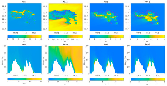
Figure 1.
Top panel: horizontal distribution of the surface mixing ratio of primary hydrocarbons RH-A and RH-B and of the corresponding organic peroxy radicals RO2-A and RO2-B calculated by the LES model for POLLUTED conditions. Lower panel: same as for the top panels, but vertical cross section at latitude 22.275 °N.
To represent the chemical fields in and around Hong Kong Island, we adopted a nested two-domain setup. The size of the outer domain is 45 km × 45 km, and the corresponding spatial resolution is 300 m. For the inner domain, whose size is 24 km × 24 km, the adopted horizontal resolution is 100 m. The height of the model top is set to 4 km altitude with 100 vertical layers for both domains. Periodic boundary conditions are used at the edge of the outer domain, which provides turbulence-inclusive boundary conditions for the inner domain [15,17].
In our simulations, the background winds are assumed to be easterlies, consistently with the prevailing winds observed in Hong Kong (about 80% of the time; see Shu et al. [18]). The initial horizontal wind velocity is equal to 10 m s−1. The topography of Hong Kong Island is added only in the inner domain, as shown in Figure 2a of the paper by Wang et al. [13]. The outer domain is assumed to be a flat area that ignores the influence of the topography and land use type.
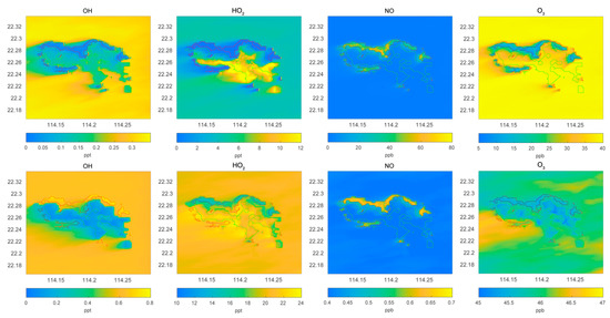
Figure 2.
Horizontal distribution of the surface mixing ratio of the hydroxyl radical OH (pptv), the peroxy radical HO2 (pptv), and the ozone molecule (ppbv). Upper panel: POLLUTED conditions; lower panel: CLEAN conditions.
5. Simulated Distribution of Chemical Species
We first show the calculated distributions of key chemical species above and around Hong Kong Island. In Figure 1, we display the surface mixing ratio calculated under polluted conditions for the anthropogenic and biogenic hydrocarbon, RH-A and RH-B, as well as their related peroxy radicals, RO2-A and RO2-B. The concentrations for RH-A are largest along the coasts, particularly in the north of the island where urban activities are most intense. In these coastal areas, the concentrations of RO2-A are the lowest, which may be because peroxy radicals are destroyed by the very abundant nitric oxide produced primarily by the intense road traffic. In the case of RH-B, the surface mixing ratios are highest near the biogenic sources in the middle of the island. The same is true for the peroxy radical RO2-B since NO concentrations are rather low in the forested areas on the mountains. When considering a cross section across the island at a specified latitude of 22.275° N, we note that the concentrations of RH-A are highest in the valleys and along the coasts, while the concentrations of RH-B are highest along the mountains. For all species, vertical mixing associated with convection in the boundary layer is intense.
We compare in Figure 2 the surface distribution of OH, HO2, NO, and ozone calculated for polluted and for clean conditions. In both simulations, NO concentrations are largest along the northern and western coasts of the island with typical mixing ratios of 50 and 0.6 ppbv for the polluted and clean cases, respectively. For both conditions, the concentrations of NO over the sea and mountains are very low. In the case of OH, the mixing ratio over the sea is of the order of 0.3 pptv in the polluted case and 0.6 pptv in the clean case. Over the mountains, the numbers are about 0.15 pptv in both cases, and along the northern coast, they are 0.05 and 0.5 pptv, respectively. In this last case, the high concentrations of RH-A and CO tend to destroy OH. In the case of HO2, the mixing ratios over the sea are higher in the clean case than in the polluted case. Along the northern coast of the island, the values are close to 1 pptv in the polluted case and 15 pptv in the clean case. Finally, the ozone concentration over the sea is in the order of 40 ppbv in the polluted case and 46 ppbv in the clean case. Near the northern coast of the island, the concentrations are about 15 ppbv in the polluted case and 45 ppbv in the clean case. Clearly, along the busy coast lines of the island, ozone is severally depleted (factor 5) due to its titration by nitric oxide. Reductions of about a factor 10 are found in the case of HO2 and OH.
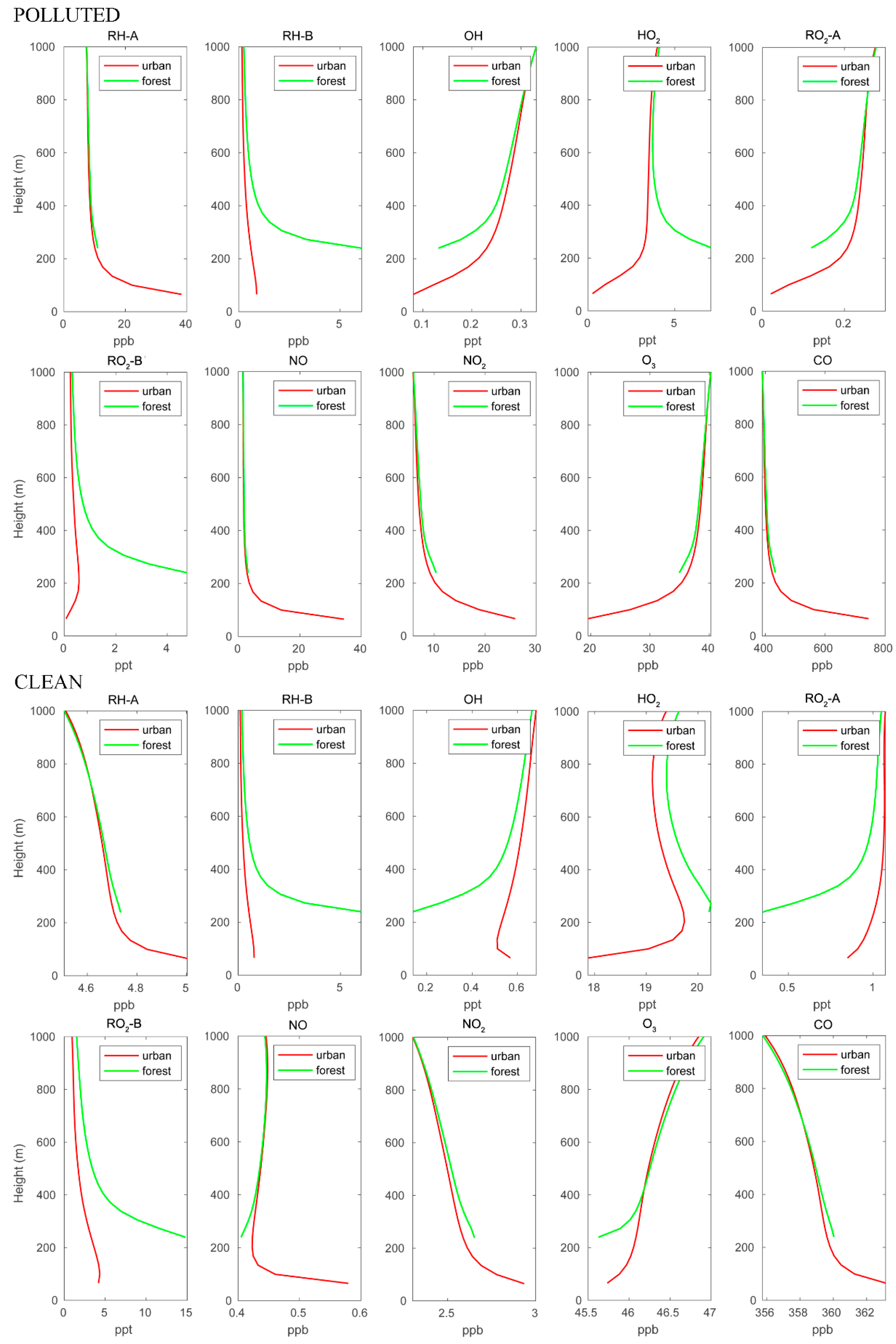
The mean vertical profiles of the different chemical species in the first kilometer of the boundary layer are shown in Figure 3. In this figure, we separate the mean profiles in the forested areas over the mountains (green curves) and over the urban settlements characterized by heavy road traffic (red curves). The graphs refer to polluted and clean situations, respectively. The vertical profiles of the anthropogenic species (RH-A, NO, and CO) are similar for both cases, with highest concentrations near the surface in the urban area. The lowest point of the profiles over the forest is located higher than that of the urban profiles because the forest is located in the mountains. The NO2 profiles share the same patterns as those of the anthropogenic species since NO2 is directly produced by conversion of NO. The biogenic compound RH-B is characterized by high concentrations at low altitudes over the mountain region, where it is emitted by the vegetation. The concentrations of RH-B are similar for the polluted and clean conditions since the biogenic emissions are assumed to be identical for both cases. The OH concentrations are lower near the surface and increase with altitude since this radical is consumed by the primary hydrocarbons (RH-A and RH-B) and by CO. These primary species are most abundant near the surface. In the polluted case, OH is depleted more effectively by RH-A and CO, and therefore, the OH concentration is lower near the urban surface, while OH is lowest at the forest ground level for the clean case. The HO2 profile in the urban area is similar to that of OH for the polluted case, but in the clean case, it exhibits a peak at about 200 m above the surface. In both cases, the HO2 vertical pattern over the forest shows a behavior opposite that of OH. The two peroxy radicals RO2-A and RO2-B, which are produced by the reaction between hydrocarbons and OH, exhibit different vertical patterns: RO2-A follows the pattern of OH, while RO2-B follows the pattern of RH-B. This is because the reaction of RH-B with OH is considerably faster than that of RH-A with OH. Ozone concentrations increase with altitudes in both cases; however, the urban surface O3 concentrations are much lower in the polluted case.
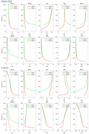
Figure 3.
Vertical distribution of different chemical species calculated over the urban and forested areas for POLLUTED and CLEAN conditions.
6. Segregation of Chemical Species
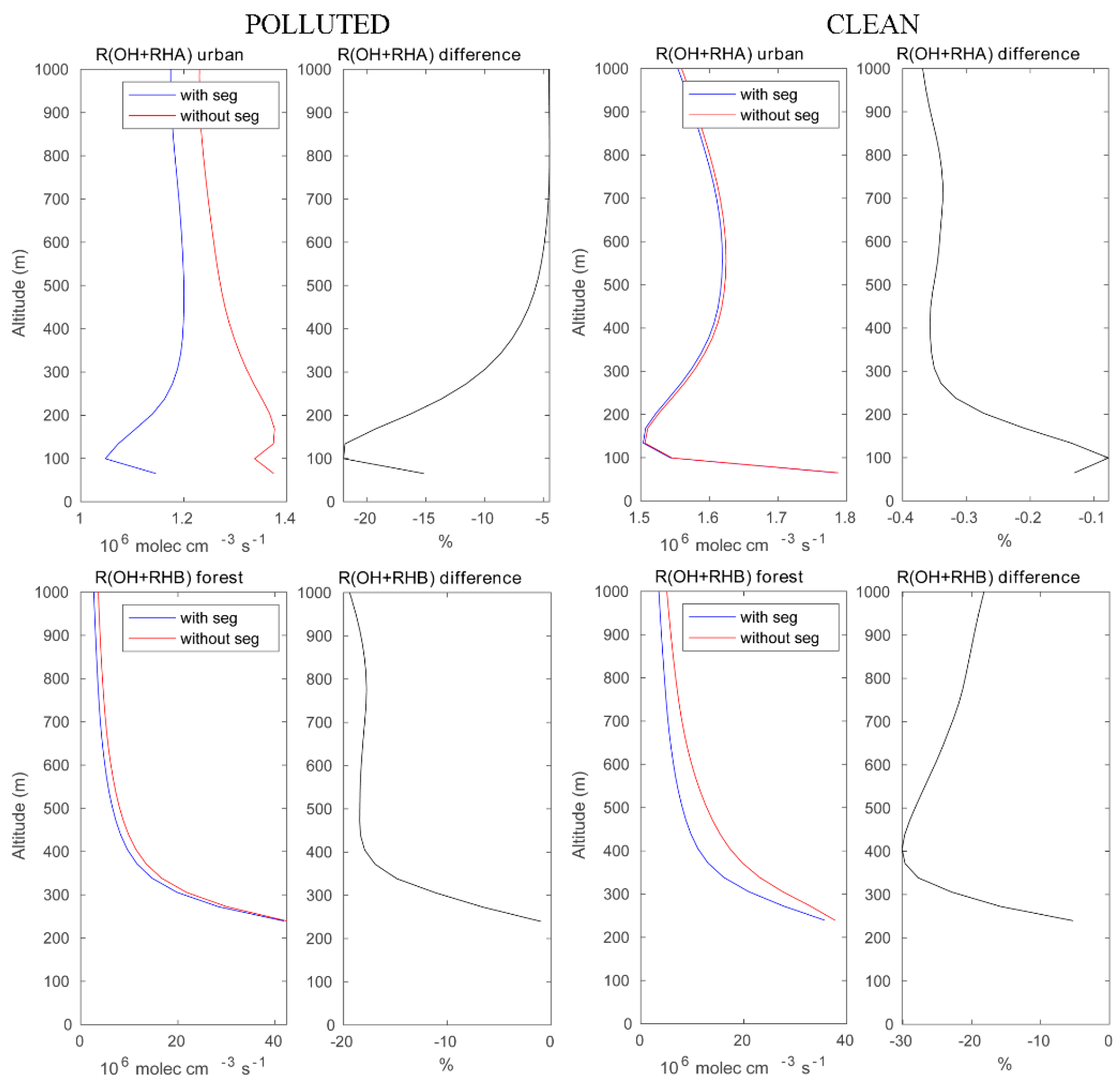
We now assess the role of segregation between chemical species in the convective boundary layer, and we discuss specifically the importance of segregation for (1) the oxidation of primary hydrocarbons by the OH radical and for (2) the photochemical formation of ozone under different chemical background environments. Figure 4 highlights the effect of segregation on the destruction rate of anthropogenic (RH-A) and biogenic (RH-B) hydrocarbons under high and low pollution conditions. The LES model shows, for example, that in urban areas with high localized NO emissions, the rate at which the reaction of RH-A by OH is substantially reduced by the segregation effect. This reduction reaches 25% at 100 m above the surface and is close to 5% above 500 m altitude. The total amount of OH destroyed by reaction with RH-A above the urban area in the boundary layer (here, we use 0–800 m to represent a large fraction of the PBL) during the selected hour is found to be 69.94 mole with segregation included and 76.77 mole with segregation ignored (see Table 2). Under assumed clean conditions, the intensity of segregation is considerably smaller (less than 1%). The OH loss by reaction with RH-A integrated over the urban area is 93.84 mole and 94.11 mole with and without segregation, respectively. The difference in the segregation intensity for RH-A and OH between polluted and clean conditions can be attributed to (1) a change in the Damköhler number resulting from the change in the emission intensities and hence in the chemical lifetime of the reactants [19,20]; and (2) a change in the primary production and loss reactions of OH associated with the different NOX regime [3]. The depletion of OH under the clean condition is higher than that in the polluted case, because the OH concentration is high. When considering the oxidation of biogenic RH-B over the forest near the mountain peaks, the segregation reduces the corresponding destruction rate by about 20–30% under both polluted and clean conditions. In the polluted case, the OH loss by RH-B integrated over the forest area is 1.26 × 10³ mole when segregation is taken into account and 1.44 × 10³ mole when segregation is ignored. In the clean case, the corresponding values are 1.37 × 10³ mole and 1.90 × 10³ mole, respectively. This is expected in a region of the island that is remote from the areas where traffic and domestic emissions are intense.
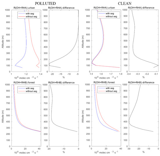
Figure 4.
Upper panels: reaction rates of OH with RH-A in the urban area with and without segregation. Lower panels: same but for the reaction of OH and with RH-B in the forested area. Left panels: polluted conditions; right panels: clean condition. The relative difference between the cases with and without segregation is equivalent to the segregation intensity.
Table 2.
Number of moles of RH-A/RH-B destroyed by OH integrated during a time period of 1 h over the lowest 20 model levels (below ~800 m) in the urban area, the forested area, and the entire domain, respectively. The results are provided for the POLLUTED and CLEAN cases. “seg” represents segregation.
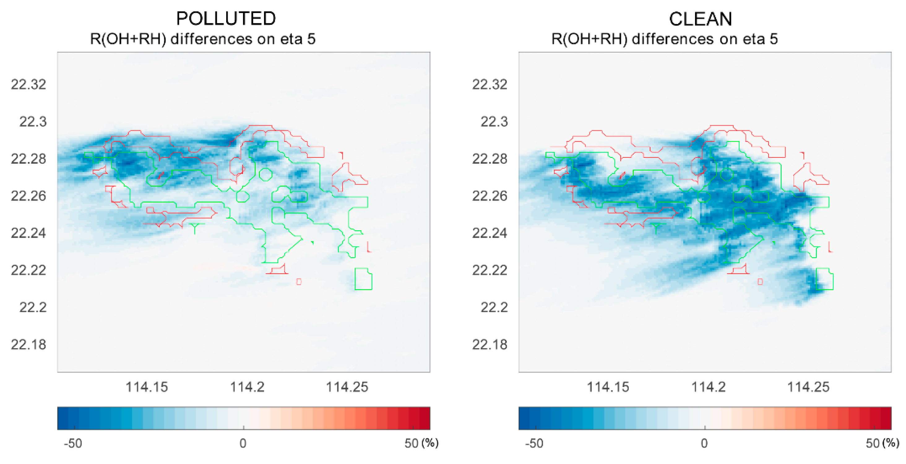
We show in Figure 5 the differences in the rate of the OH – RH reaction between cases with and without segregation. This figure combines the destruction rate of OH by RH-A and RH-B. We can see that under the polluted conditions, segregation has a larger impact at the north coast of the island where the anthropogenic emissions are the largest. However, under clean conditions, the segregation-induced differences become smaller in the urban region; in this case, the impact is even stronger over the forest area than that for the polluted case. Previous studies show large discrepancies in OH concentrations in the tropics between observations and models, and attribute these discrepancies to the fact that the effect of segregation has been ignored in the coarse models [21]. Subsequent studies such as those of Ouwersloot et al. point out that segregation only changes the calculated OH budget within a limited range [22]. However, our simulations suggest that segregation plays a significant role in the OH – RH-B reaction. Additionally, segregation has a large impact on the OH – RH-A reaction in the polluted region, even though the reaction rate between OH and RH-A is much slower than that of OH and RH-B. In our case, the NO levels did not affect the OH – RH-B reaction much, because the urban and forest regions are separated by the mountains, and the NO concentrations are low over the forest in both polluted and clean cases.
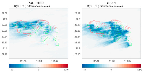
Figure 5.
The differences in the reaction rates of OH with hydrocarbons (RH-A and RH-B) at model level 5 (approximately 200 m above ground) with and without segregation. Left panel: polluted conditions; right panel: clean conditions.
Finally, we examine the role of segregation in the production rate of ozone. As we retain in our simple chemical mechanism two hydrocarbons (RH-A and RH-B), and thus two peroxy radicals (RO2-A and RO2-B), the ozone production rate from Equation (7) becomes:
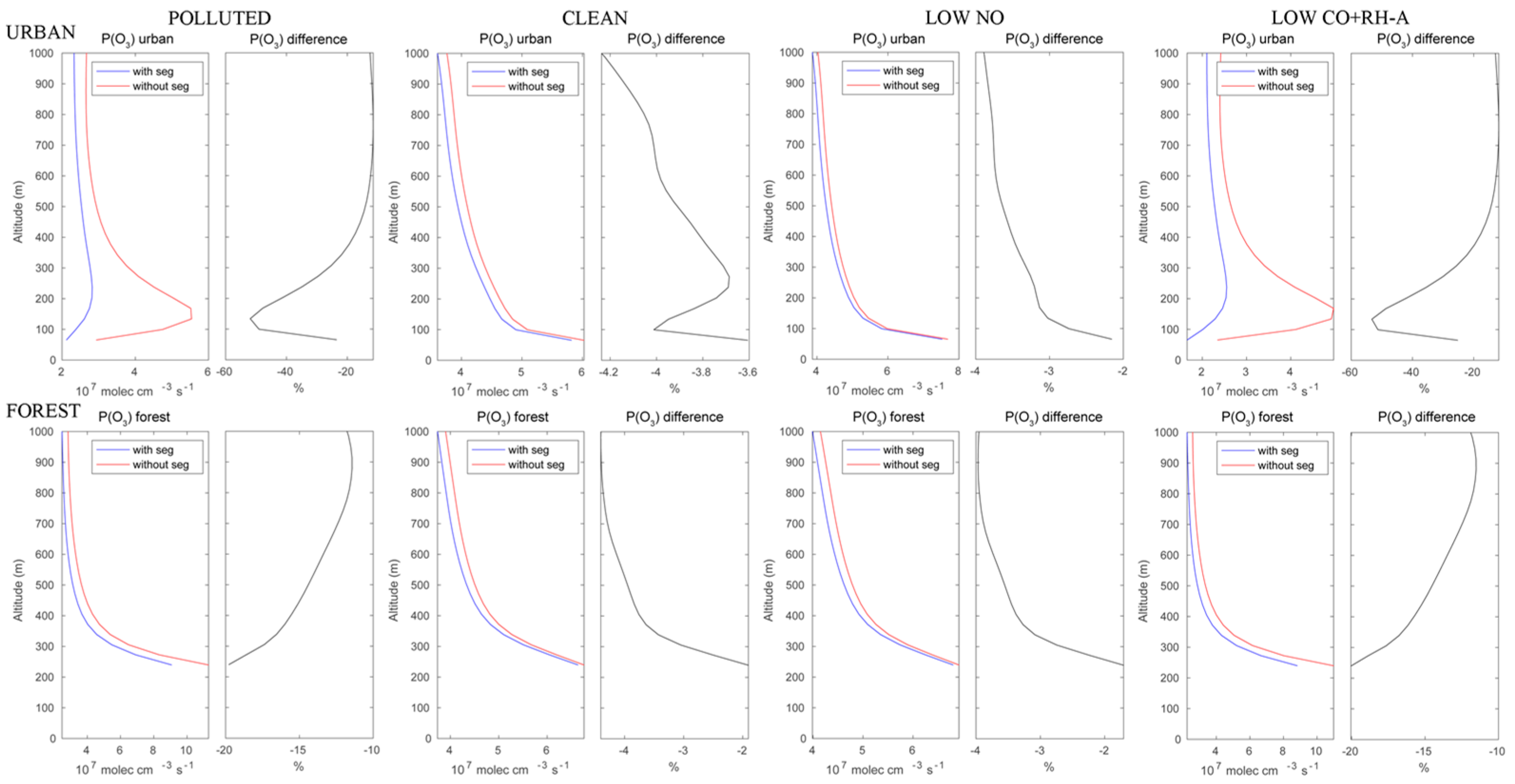
The calculated ozone production rates are shown in Figure 6. In the urban area under polluted conditions, the reduction in the ozone formation rate reaches 50% at about 150 m above the surface and decreases to less than 20% above the height of 500 m. Under assumed clean conditions, this reduction due to segregation would be only of the order of 4% in the boundary layer. In the forested areas of the Hong Kong Island mountains, the reduction in the ozone production rate would decrease from about 20% near the surface to 12% at 1000 m altitude. Under clean conditions, the reduction is considerably smaller and increases from 2% to 4% with height.

Figure 6.
Upper panels: production rate of ozone in the urban area with and without segregation. Lower panels: same but for the forested areas. First columns: polluted conditions; second columns: clean conditions; third columns: low NO conditions; fourth columns: low CO+RH-A conditions. The relative difference is a measure of the effect of segregation.
Besides the polluted and clean cases discussed above, two additional simulations were performed to provide sensitivity tests. One assumes low NO emissions corresponding to the CLEAN case, while the emissions of CO and RH-A remained as in the POLLUTED case. In the second case, CO and RH-A emissions were set at the values of the CLEAN case, while the emission of NO remained high at the POLLUTED levels. The ozone production rates resulting from these two cases are shown in Figure 6.
The ozone production patterns for the low NO case are very similar to those of the clean case. The case with high NO but low CO and RH-A shows patterns similar to those found in the polluted case. This suggests that in our simple model conditions, the ozone production is limited by the NO levels rather than the other anthropogenic species.
7. Conclusions
We have shown that turbulent motions affect the rate at which chemical species react together and hence their mean concentration in the planetary boundary layer. Segregation effects can only be captured in high-resolution models and quantified, for example, through large eddy simulations. The effect of segregation is best quantified by the so-called segregation intensity, which is equivalent to the relative change due to segregation of the reaction rate. The methodological approach summarized in the first section of this paper was applied to Hong Kong Island. This area is subject to strong turbulent motions and is characterized by inhomogeneous emissions of chemical species. To avoid excessive computational burden in a conceptual study, the adopted chemical mechanism was idealized with two primary hydrocarbons, one of anthropogenic origin emitted in the urbanized areas, mostly along the coasts, and the second one of biogenic origin emitted by the vegetation on the mountains. We also considered a polluted case, intended to mimic the current situation, and a clean case, intended to be representative of the city that has taken drastic action to improve air quality.
The numerical simulations show that the concentrations of the chemical compounds are quite different along the coast of the island and over the mountains, which are dominated by urban and forest emissions, respectively. The reduction in the anthropogenic emissions modifies not only the concentrations of the emitted chemical species but also the distribution patterns of some compounds such as OH and O3.
The reduction in the reaction rate of OH and RH-A by segregation reaches 25% near the surface in urban areas under heavy pollution conditions; however, the influence of segregation becomes considerably smaller under clean conditions. The segregation effect reduces by 20–30% the rate of the reaction between OH and RH-B in both polluted and clean cases. If we combine the effects of anthropogenic and biogenic hydrocarbons, the impact of segregation is greater in urban areas under high pollution, and under clean conditions, it is greater in forested areas.
The ozone production rate is also influenced by segregation. Under polluted conditions, segregation reduces the ozone production rate by as much as 50% at about 100 m above the urban region, and by 20% near the surface of the forested mountain area. The effect of segregation is considerably smaller under clean conditions. When the sources of anthropogenic species are reduced by a factor of 100, the reduction in the ozone production rate is only of the order of 2–4% in both urban and forest regions. Two addition sensitive runs with low NO or low RH-A and CO were conducted to estimate the factors that affect ozone production. The results show that with our setup, the NO source strength is the dominant factor that controls ozone production as well as the segregation impact level on the ozone production rate.
We conclude that in urban areas with inhomogeneous emissions of pollutants affected by turbulent flows, segregation between fast-reacting species can be substantial and affects the rate at which photochemistry operates. This seems the case, particularly for the rate at which primary hydrocarbons are oxidized and the rate at which boundary layer ozone is produced. It is therefore advisable, when considering urban chemistry in a multi-scale global and regional modelling environment, to implement a zooming capability to address segregated processes in urban areas. The new generation of models such as the MUSICA (the Multi-Scale Infrastructure for Chemistry and Aerosols) platform currently under development that includes an unstructured grid with regional refinement is an important step in this direction [23]. It could be complemented in the future by considering additional zooming capabilities that would resolve turbulent-scale processes at tens of meters resolution in urban settings.
Author Contributions
Conceptualization, G.P.B.; methodology, Y.W. and G.P.B.; software, Y.W.; validation, Y.W.; formal analysis, Y.W.; investigation, Y.W. and G.P.B.; resources, Y.W.; data curation, Y.W.; writing—original draft preparation, Y.W.; writing—review and editing, G.P.B. and T.W.; visualization, Y.W.; supervision, G.P.B. and T.W.; project administration, T.W.; funding acquisition, T.W. All authors have read and agreed to the published version of the manuscript.
Funding
This research was funded by the Hong Kong Research Grants Council (grant no. T24-504/17-N) and the National Natural Science Foundation of China (NSFC award no. 42075078).
Institutional Review Board Statement
Not applicable.
Informed Consent Statement
Not applicable.
Data Availability Statement
The data presented in this study are available on request from the corresponding author.
Acknowledgments
We would like to acknowledge Domingo Muñoz-Esparza and Mary Barth from NCAR for the constructive discussions and technical help. High-performance computing support was provided by the NCAR Cheyenne cluster.
Conflicts of Interest
The authors declare no conflict of interest.
References
- Stevenson, D.S.; Zhao, A.; Naik, V.; O’Connor, F.M.; Tilmes, S.; Zeng, G.; Murray, L.T.; Collins, W.J.; Griffiths, P.T.; Shim, S.; et al. Trends in global tropospheric hydroxyl radical and methane lifetime since 1850 from AerChemMIP. Atmos. Chem. Phys. 2020, 20, 12905–12920. [Google Scholar] [CrossRef]
- Kim, S.W.; Barth, M.C.; Trainer, M. Influence of fair-weather cumulus clouds on isoprene chemistry. J. Geophys. Res. Atmos. 2012, 117, D10302. [Google Scholar] [CrossRef] [Green Version]
- Kim, S.W.; Barth, M.C.; Trainer, M. Impact of turbulent mixing on isoprene chemistry. Geophys. Res. Lett. 2016, 43, 7701–7708. [Google Scholar] [CrossRef] [Green Version]
- Deardorff, J.W. A numerical study of three-dimensional turbulent channel flow at large Reynolds numbers. J. Fluid Mech. 1970, 41, 453–480. [Google Scholar] [CrossRef]
- Smagorinsky, J. General circulation experiments with the primitive equations: I. The basic experiment. Mon. Weather Rev. 1963, 91, 99–164. [Google Scholar] [CrossRef]
- Wyngaard, J.C. Turbulence in the Atmosphere; Cambridge University Press: Cambridge, UK, 2010; p. 405. [Google Scholar]
- Dai, Y.; Cai, X.; Zhong, J.; MacKenzie, A.R. Modelling chemistry and transport in urban street canyons: Comparing offline multi-box models with large-eddy simulation. Atmos. Environ. 2021, 264, 118709. [Google Scholar] [CrossRef]
- Kim, Y.; Wu, Y.; Seigneur, C.; Roustan, Y. Multi-scale modeling of urban air pollution: Development and application of a Street-in-Grid model (v1.0) by coupling MUNICH (v1.0) and Polair3D (v1.8.1). Geosci. Model Dev. 2018, 11, 611–629. [Google Scholar] [CrossRef] [Green Version]
- Vinuesa, J.F.; Vilà-Guerau de Arellano, J. Introducing effective reaction rates to account for the inefficient mixing of the convective boundary layer. Atmos. Environ. 2005, 39, 445–461. [Google Scholar] [CrossRef]
- Danckwerts, P.V. The definition and measurement of some characteristics of mixtures. Appl. Sci. Res. 1952, 3, 279–296. [Google Scholar] [CrossRef]
- Wang, T.; Xue, L.; Brimblecombe, P.; Lam, Y.F.; Li, L.; Zhang, L. Ozone pollution in China: A review of concentrations, meteorological influences, chemical precursors, and effects. Sci. Total Environ. 2017, 575, 1582–1596. [Google Scholar] [CrossRef]
- Damköhler, G. Der Einfluss der Turbulenz auf die Flammengeschwindigkeit in Gasgemischen (Influence of turbulence on the velocity of flames in gas mixtures). Z. Elektrochem. Angew. Phys. Chem. 1940, 46, 601–626. [Google Scholar]
- Wang, Y.; Ma, Y.-F.; Muñoz-Esparza, D.; Li, C.W.Y.; Barth, M.; Wang, T.; Brasseur, G.P. The impact of inhomogeneous emissions and topography on ozone photochemistry in the vicinity of Hong Kong Island. Atmos. Chem. Phys. 2021, 21, 3531–3553. [Google Scholar] [CrossRef]
- Skamarock, W.C.; Klemp, J.B.; Dudhia, J.; Gill, D.O.; Liu, Z.; Berner, J.; Wang, W.; Powers, J.G.; Duda, M.G.; Barker, D.M.; et al. A Description of the Advanced Research WRF Model Version 4; NCAR: Boulder, CO, USA, 2019; p. 145. [Google Scholar]
- Moeng, C.H.; Dudhia, J.; Klemp, J.; Sullivan, P. Examining two-way grid nesting for large eddy simulation of the PBL using the WRF model. Mon. Weather Rev. 2007, 135, 2295–2311. [Google Scholar] [CrossRef]
- Deardorff, J.W. Stratocumulus-capped mixed layers derived from a three-dimensional model. Bound.-Layer Meteorol. 1980, 18, 495–527. [Google Scholar] [CrossRef]
- Muñoz-Esparza, D.; Kosović, B.; García-Sánchez, C.; van Beeck, J. Nesting turbulence in an offshore convective boundary layer using large-eddy simulations. Bound.-Layer Meteorol. 2014, 151, 453–478. [Google Scholar] [CrossRef]
- Shu, Z.R.; Li, Q.S.; Chan, P.W. Statistical analysis of wind characteristics and wind energy potential in Hong Kong. Energy Convers. Manag. 2015, 101, 644–657. [Google Scholar] [CrossRef]
- Molemaker, M.J.; Vilà-Guerau de Arellano, J. Control of chemical reactions by convective turbulence in the boundary layer. J. Atmos. Sci. 1998, 55, 568–579. [Google Scholar] [CrossRef]
- Li, C.W.Y.; Brasseur, G.P.; Schmidt, H.; Mellado, J.P. Error induced by neglecting subgrid chemical segregation due to inefficient turbulent mixing in regional chemical-transport models in urban environments. Atmos. Chem. Phys. 2021, 21, 483–503. [Google Scholar] [CrossRef]
- Butler, T.M.; Taraborrelli, D.; Brühl, C.; Fischer, H.; Harder, H.; Martinez, M.; Williams, J.; Lawrence, M.G.; Lelieveld, J. Improved simulation of isoprene oxidation chemistry with the ECHAM5/MESSy chemistry-climate model: Lessons from the GABRIEL airborne field campaign. Atmos. Chem. Phys. 2008, 8, 4529–4546. [Google Scholar] [CrossRef] [Green Version]
- Ouwersloot, H.G.; Vilà-Guerau de Arellano, J.; van Heerwaarden, C.C.; Ganzeveld, L.N.; Krol, M.C.; Lelieveld, J. On the segregation of chemical species in a clear boundary layer over heterogeneous land surfaces. Atmos. Chem. Phys. 2011, 11, 10681–10704. [Google Scholar] [CrossRef] [Green Version]
- Pfister, G.G.; Eastham, S.D.; Arellano, A.F.; Aumont, B.; Barsanti, K.C.; Barth, M.C.; Conley, A.; Davis, N.A.; Emmons, L.K.; Fast, J.D.; et al. The multi-scale infrastructure for chemistry and aerosols (MUSICA). Bull. Am. Meteorol. Soc. 2020, 101, E1743–E1760. [Google Scholar] [CrossRef]


Publisher’s Note: MDPI stays neutral with regard to jurisdictional claims in published maps and institutional affiliations. |
© 2022 by the authors. Licensee MDPI, Basel, Switzerland. This article is an open access article distributed under the terms and conditions of the Creative Commons Attribution (CC BY) license (https://creativecommons.org/licenses/by/4.0/).