Abstract
As global warming produces dramatic climate changes, water management is facing increasingly serious challenges. Given to the process of climate change and its complex effects on watershed hydrology, this paper investigates the spatial and temporal variation characteristics of major climatic factors (i.e., precipitation and temperature) over the upper Yangtze River basin (UYRB), China. The statistical analyses are based on annual and seasonal scales during 1951–2020 with a recorded period of seven decades. The Mann–Kendall nonparametric test and R/S analysis are used to record the temporal trends (past and future) of climate variables; the Pettitt test, standard normal homogeneity test and Buishand test are used to detect the homogeneity in climate series. The sensitivities of the streamflow to climatic parameters are assessed at the watershed scale, especially considering the Three Gorges Dam’s (TGD) effect on changing runoff. The results of the study indicate that the annual precipitation of 29 out of 34 series indicate homogeneity, while 31 out of 34 annual mean temperature series show heterogeneity, with jump points around 1997 in the mean temperature of 20 sites. Detectable changes in precipitation were not observed during 1951–2020; however, the temperature increased significantly in the whole basin on annual and seasonal scales, except for several stations in the eastern part. The magnitude of increase in air temperature in high altitudes (Tibet Plateau) is higher than that in low altitudes (Sichuan Plain) over the last seven decades, and future temperatures continue to sharply increase in high altitudes. The TGD plays an important role in explaining the seasonal variations in streamflow at Yichang station, with streamflow experiencing a sharp increase in winter and spring (dry season) and a decrease in summer and autumn (rainy season) compared to the pre-TGD period. The streamflow variation at an annual scale is mainly regulated by climate fluctuation (variation in precipitation). During the last seven decades, increasing air temperature and decreases in rainfall and runoff signify reduced water resources availability, and the climate tends to be warmer and drier over the basin. The sensitivity of the streamflow to watershed precipitation is higher than that to temperature, with variation in annual rainfall explaining 71% of annual runoff variability.
1. Introduction
Unprecedented changes in the global climate system have occurred since the 1950s [1]. According to the fifth assessment report of the Intergovernmental Panel on Climate Change (IPCC), the annual mean temperature from 2003 to 2012 increased by 0.78 °C compared with that from 1850 to 1900 [2]. Climate Change is no doubt one of the major challenges facing the human race today [3]. The most obvious impacts of climate change have resulted in the rise in global temperatures and altered precipitation patterns [4,5]. Due to the inseparable linkage between the climatic and hydrological cycle, global warming is reported to accelerate water circulation, which will lead to spatio-temporal redistribution of water resources at global and regional scales [6,7,8,9,10,11].
Temperature and precipitation are fundamental components of climate, and the analysis of changes in these variables characterizes key task in detecting climate changes [12]. Rising global surface temperatures are likely to cause changes in atmospheric circulation, accelerate the hydrological cycle and increase the water holding capacity throughout the atmosphere [13,14,15]. Spatial and temporal patterns of water availability are also influenced by rainfall as the critical component of hydrologic cycle [7,16]. Variation in precipitation directly or indirectly affects water resources management, fresh water availability and both droughts and floods events [6,7,17,18]. One of the challenges posed by climate change is the ascertainment, identification and quantification of trends in these climatic variables and their implications on river flows so as to assist in the formulation of adaptation measures through appropriate strategies for water resources planning and management [19,20]. Information regarding hydroclimatic issues is crucial within the context of water cycles, global warming and increasing demand for water as a result of urbanization and economic growth [21]. Accordingly, understanding variations and trends of historical hydroclimatic variables are relevant to the future development and sustainable water resources management of a given region.
The intensive research in recent years on climate change has led to the strong conclusion that climate has always, throughout the Earth’s history, changed irregularly on all time scales [22]. Global climate change affects precipitation and temperature differently in different parts of the world [18]. IPCC has indicated the necessity of trend analysis for the assessment of climate change [23]. The climate variability, anthropogenic or natural, increases the uncertainty of hydrological processes [22]. Climate change impacts are bound to cause unexpected modifications on the hydrological system components in the forms of increasing (decreasing) trends, intensification in the occurrence frequency and magnitude variations [24]. Understanding the variations of rainfall, temperature and runoff at the basin scale provides an opportunity to evaluate the changing climate’s impact on the hydrological cycle [12], while realizing possible hydrological behavior under climate variability is of utmost importance for effectively addressing water resources issues [3]. In addition, the detection and attribution of past trends, changes and variability in hydroclimatic variables are favorable for understanding potential future changes resulting from anthropogenic activities [25].
Under the combined impacts of climate change and human activities, the stability of hydrological sequences has already been changed [3]. The hydrologic regime of a stream under specific geomorphic conditions represents the integrated basin response to various climatic inputs, with precipitation and temperature being very important [25]. Milly et al. defines stationarity as the idea that natural systems fluctuate within an unchanging envelope of variability [26]. There is an implicit assumption of stationarity, implying time-invariant statistical characteristics of the time series under consideration in virtually all water resources engineering works. Such an assumption will no longer be valid if the global climate changes as a result of the increase in greenhouse gases in the atmosphere [27]. It has been documented that quasi-periodic climate behavior and systematic trends of key climate variables attribute to climate change [28]. An important element of the research on the impacts of climatic change is the analysis of trends in hydrological variables providing insights into the characteristics and magnitude of regional climatic variations [29,30]. Given this in mind, the trend characteristics of hydrological variables might be used as indicators to monitor climate change and evidences of climate variability [31].
Understanding the spatial and temporal variability of rainfall and temperature is challenging and requires high-quality observed datasets [12]. Many types of disturbances can cause apparent changes in long-term climatological time series, which may distort the true climatic signal [32]. One of the most important characteristics of a climatic time series is homogeneity [18]. A homogeneous climate data series is defined as one where variations are caused only by variations in weather and climate [33]. Breaks in the homogeneity of time series may be caused by nonclimatic factors, such as changes in instruments, observation methods, station locations, environments, etc., during the history of meteorological stations that make climate data unrepresentative of temporal climate variability [20,32,34]. Recently developed statistical techniques are available for detecting the presence of long-term movements in recorded time series so as to test the homogeneity problems [35]. As mentioned by Hall [36], even when the timing and duration of an apparent trend have been quantified, a decision is required on its authenticity: Could the movement be a reflection of long-term climate variability, or is it an artifact of the instrumentation or its environment?
It is known that the Yangtze River is the largest river in China and the third-largest river in the world [37]. With its rich natural resources, diverse economic culture and important location advantages, the Yangtze River Basin (YRB) has occupied an extremely important position in China’s social and economic development [38]. The YRB is home to one-third of the country’s population, and the largest capacity hydropower project in the world to date is the Three Gorges Dam (TGD) located at the end of the upper reaches [39]. The Yangtze River is extraordinarily vulnerable to climate warming due to its dense population and the rapidly developed economy [33]. A majority of extreme temperature indices appear as abrupt changes since the last decades, with the main cold indices changing abruptly in the 1980s and the main warm indices changing abruptly in the late 1990s and early 2000s [40]. The maximum and minimum temperatures have increased significantly at rates of 0.19 °C and 0.37 °C per decade, respectively [41]. A recent study has reported that the magnitude of the changes in extreme climate events in the Yangtze River basin is projected to increase with the increasingly warming climate [42]. These variations have exerted a considerable influence on society and the ecosystem, making climate change one of the most urgent challenges facing the YRB [40].
According to the Fifth Assessment Report (FAR5) of the IPCC, numerous evidences have corroborated shifts in weather and hydrologic events toward the extreme side since the 1950s [43]. Rainfall is the most vital climatic variable, owing to its manifestation as a deficient resource (droughts) or a catastrophic agent (floods) [44]. A recent study has indicated that the upper Yangtze River basin is facing increasing droughts [3]. Coupled with this, since the 21st century, several regional extreme events have occurred in the Yangtze River Basin, resulting in a large number of deaths and economic losses [45]. These losses helped to raise the alarm over the possibility that the extreme events were caused by climate change [44]. However, one of the most important necessities of research into climate change is to analyze and detect historical changes in the climatic system [44]. In addition, the spatial and temporal distribution of precipitation governs the ecohydrological processes [46]. Changes in temperature and precipitation caused by climate change will affect vegetation growth and the temporal and spatial distribution of water resources [47]. An unbalanced distribution of precipitation implies the emergence of drought, while a low soil humidity results in the devastation of vegetation cover [48]. In this context, human living environments and natural ecosystems will be notably altered by vegetation change. The variability and availability of water resources also have direct influences on local eco-environmental conservation and sustainable socioeconomic development [49]. Reduced water availability and drought are identified as the main factors limiting tree growth in a region [50]. The Yangtze River Basin (YRB) is rich in vegetation types and has functions such as water and soil conservation and regulation of river runoff [38]. There are alpine meadows and alpine grasslands in the upper reaches, and subtropical evergreen broad-leaf forests in both the eastern and western parts of the basin [51]. The assessment of climate change is therefore important, especially considering that the unique ecosystems of the basin may be highly affected by extreme climate events such as droughts [50].
A substantial number of long hydroclimatic time series exhibit Hurst phenomena. Simple scaling processes offer a stochastic basis for dealing with these shifts and trends, and such processes are consistent with the assumption of hydroclimatic fluctuations on multiple time scales, a behavior that is called the Hurst phenomenon [22]. As stated by Koutsoyiannis [22], in time series with short length, the classical statistics can hide the scaling behavior. That is to say, the short time series classified as random noise without scaling behavior may actually exhibit the Hurst phenomenon. A statement consistent with this is that the ability of nonparametric tests to detect existing trends is significantly influenced by sample size or record length [52]. The larger the sample size, the more powerful the test. These descriptions emphasize the significance of a sufficient length of time series to understand the features and magnitudes of recent climatic changes [53]. Observational findings based on relatively short periods cannot be considered as a sufficient evidence of climate change [33]. As proposed by Kundzewicz and Robson [54], given the climate variability, at least 50 years of records are necessary for climate change detection. Here, we investigate a 70-year window (1951–2020) of observations from a network of 34 meteorological stations and the hydrologic control station of the UYRB. The statistical period of datasets forms an excellent foundation for the trend detection studies.
Spatial variability in the long-term behavior of climate is dependent on regional and local characteristics [16]. Climate trends at the regional scale are by no means easy to detect, since regional climate has relatively greater variability associated with natural climatic processes [35]. Autocorrelation is recognized to be quite common in temperature and precipitation time series and may affect the computation of linear trends [55]. This study attempts to produce more reliable estimates of trend magnitude and the statistical significance by taking into account the autocorrelation detected in climate time series. Sequentially to this, conducting relatively small-scale analyses and a check for inhomogeneity are of great importance to avoid biases, spurious trends and erroneous interpretations from the data series used for such analyses [16]. In view of this, this paper focuses on investigating the trends and homogeneities in hydroclimate series in the UYRB to analyze whether there are significant trends and long-term movements (i.e., jumps in the mean) in precipitation and temperature as previous studies of this basin did not focus on this. This study also focuses on whether there is a Hurst phenomenon in watershed-scale climate variables to estimate the persistence of future trends. In addition, the sensitivities of runoff as a vital hydrological variable to long-term climatic parameters are also focused in this study. This study is necessary since the enormous importance of the basin to sustaining the livelihood of the inhabitants and also its general water resources contribution to the well-known Three Gorges Dam.
The present study aims to detect the long-term variations in hydroclimatic variables over the UYRB. The main objectives are: (i) to examine temporal trends in rainfall and temperature with their spatial patterns on annual and seasonal scales; (ii) to detect the possible long-term movements and step-changes in climatic and hydroclimatic parameters in the UYRB; and (iii) to analyze the relationships between streamflow and climatic variables so as to initially clarify the impacts of climatic changes on water resources. This study will provide a baseline to which future analyses of variability and trends in hydroclimatic variables over the UYRB can be compared. The findings of this paper can provide insights and guidance to the effects of variations in rainfall and temperature on surface-water resources and provide useful information for the long-term planning and management of water resources in the upper Yangtze River.
2. Study Site and Climatic Data
2.1. Study Site
The Yangtze River originates from the Qinghai–Tibet Plateau and runs through the Mainland of China to the East China Sea [56]. With a total length of 6300 km, it is the longest river in Asia and the third longest river in the world [57]. The Upper Yangtze River Basin (UYRB, Figure 1) covers the area of 24.30–35.45 N and 90.33–112.04 E, originating from headwaters to Yichang gauging station located just downstream of the TGD [58]. The UYRB has a length of 4529 km and a controlled drainage area of 1,000,000 km [59], accounting for 58.9% of the total basin area of the Yangtze River [60]. The upper catchment contains four major tributaries, i.e., Jinshajiang, Mintuojiang, Jialingjiang and Wujiang, and the main stream of the upper reaches [61]. The climate is characterized by complex regional sub-basin-scale patterns of precipitation and temperature in terrain ranging from plateaus to plains [39]. The watershed climate is mainly influenced by the Indian Summer Monsoon, and the climate is drier and colder at the western end of the upstream [58]. With a typical subtropical monsoon climate, most of the areas in the UYRB are warm and humid [57]. The mean annual rainfall ranges from 800 mm to 1000 mm over the basin, although the annual rainfall may reach up to 1560 mm in some local regions, such as the middle Sichuan Basin, and lower than 500mm in some regions in the west [59]. The spatial distribution of rainfall is extremely uneven; in general, the rainfall decreases from the southeast to the northwest of the catchment [62]. The watershed has a vast territory, diverse landform types and high western and low eastern elevations [63]. The topographic difference across the basin exerts great influence on climate, e.g., the annual mean temperature is in the range from 0 to 17 C between the Tibetan Plateau and the Sichuan Basin [62], leading to the diversity of hydroclimatic conditions in UYRB [56]. More than 60% of annual rainfall is concentrated in summer, which causes flooding frequently, as well as droughts sometimes, in the basin [61]. The upper reaches of Yangtze River, as the freshwater source for the middle and lower Yangtze, is extremely vulnerable to climate variation [60]. Understanding the spatio-temporal variability of hydroclimatic parameters in UYRB can provide helpful information to creating appropriate water resource adaptation policies and strategies under a changing climate.
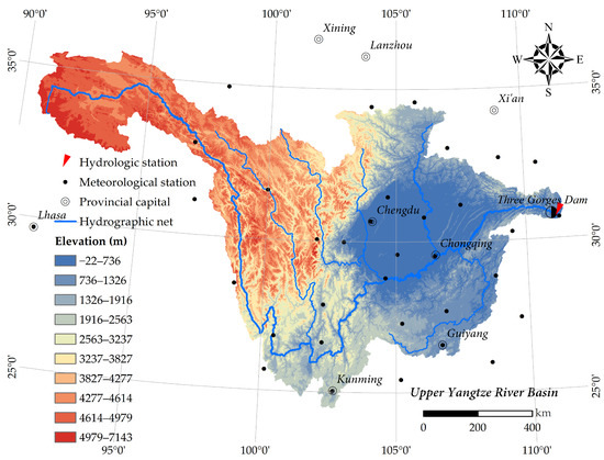
Figure 1.
Topographic map of the upper Yangzte River basin (UYRB) and distribution of gauging stations.
2.2. Climatic Data
Monthly precipitation and temperature time series were derived from the National Climate Center of the China Meteorological Administration (http://cmdp.ncc-cma.net/cn/download.htm, accessed on 21 October 2021). The 34 meteorological stations used in this study are located in and around the upstream Yangtze river, with continuous observations spanning the period of 1951 to 2020. As the longest records that were made available, no missing values exist in the seven decades. Datasets were processed following strict quality-control procedures conducted by the National Climatic Center of China’s Meteorological Administration that could ensure completeness and accuracy. Annual series were prepared for each station, and trend analysis was performed on the annual scale. The monthly rainfall and temperature data were divided into winter (December, January and February), spring (March, April and May), summer (June, July and August) and autumn (September, October and November) for seasonal analysis. The daily runoff records of Yichang station, the exit control hydrologic station of the UYRB, were collected from the Hydrological Year Book published by the Hydrology Bureau of Yangtze River Water Resources Commission. Data series cover the period of 1951–2020 without any gaps or missing values. The monthly averaged flow data were obtained by averaging the daily flow rates within each month. The annual and seasonal series were prepared from monthly datasets, with runoff in monsoon summer (June, July and August) dominated [39]. The runoff data were converted to millimeter units by using the catchment area of Yichang station for subsequent analysis.
The geographic distribution of the selected gauging stations is presented in Figure 1. The meteorological stations are unevenly distributed across the UYRB, with a slightly lower concentration on the eastern Tibetan Plateau. These descriptions highlight the potential uncertainty of the study results, especially for areas with few meteorological stations. The management of water resources has been subject to a variety of sources of uncertainty, not least of which has been the natural variability of the climate [36]. Precipitation patterns in most cases dictate the hydrological regime of river basins [16]. However, such considerations are compounded by the possible effect of anthropogenically related hydrological processes. Climate change and human activities jointly affect the hydrological variations of watershed [64]. Due to the nonlinear behavior of hydrological processes and the effects of dam construction, it is difficult to adequately relate hydrological changes to climate signals by analyzing observed changes in precipitation and runoff alone, especially for the main stream [61]. The Yichang station is known as Gateway to the Three Gorges and is located approximately 40 km downstream of the dam [39]. Hydraulic structures on rivers, such as the Three Gorges Dam (TGD), can alter the river flow to a large extent [61], signifying changes in precipitation cannot easily be converted into amounts of observed streamflow change. Given this in mind, this study considers the hydrological effects in the upper Yangtze River under natural climate change, particularly in the context of the intense impact of the TGD.
The investigation of climate change places a premium on long and homogeneous instrumental records of both hydrological and hydrometeorological variables [36]. A sufficient length of time series is crucial to be able to distinguish between natural climate variability and signals of climate change [11,54]. The statistical period is an important factor in hydrologic and climatic investigations [65]. Climate variability can easily give rise to apparent trends when statistical periods are short; these are trends that would be expected to disappear once more data had been collected [54]. The greater the statistical period, i.e., the longer the period data of one parameter are available, the more precise and reliable the analysis [65]. In this instance, the period of seven decades from 1951 to 2020 provides the most reliable time to compare rainfall, temperature and runoff trends. Meanwhile, a high quality of time series is required to prevent non-climatic factors, such as changes in observation practices or site relocation, from affecting the determination of trends [32]. Inhomogeneities in climatic series may be introduced by an abrupt change (or jump), by a gradual trend or by a jump superimposed on a trend [20,54]. That is to say, the inhomogeneity in the data produces either sharp discontinuities or gradual deviations [20]. Available literature documented that heterogeneous precipitation and temperature series would have been systematically biased, and inhomogneities of individual time series may be as great as the decadal variations of climate [32]. Unfortunately, long time series normally exhibit inconsistencies and non-homogeneities due to a wide variety of causes [36]. When adopting strict criteria regarding data length and data quality, the number of stations suitable for analysis strongly decreases. However, a small database limits the significance of attained results [11]. Homogeneity tests can be used to detect the presence of long-term movements in recorded time series, but the interpretation of the results from such tests is often conducted in the absence of sufficient station metadata [36]. Various changes during the history of meteorological stations can be the cause of loss of climate series homogeneity [34]. Such information is not readily available; however, even if a station history is available, the adjustment of suspect records generally requires the deployment of more sophisticated algorithms, as stated by Peterson et al. [66]. As indicated by Hall [36], the results of statistical testing for inconsistency and non-homogeneity should also be interpreted in the context of prevailing weather systems. In this regard, it is important to objectively consider and attribute the results of these tests, especially in the broader context of regional weather systems and their variability.
3. Methodology
To carry out the purpose of this paper, the following methods were used: (1) Significance of autocorrelation was detected by using Student’s t-test at lag 1 for annual and seasonal series. (2) Mann–Kendall (MK) and Modified Mann–Kendall (MMK) tests were applied to non-autocorrelated and autocorrelated series to detect the trends and significance, respectively. (3) Trend magnitudes were estimated by Theil–Sen’s slope estimator. (4) Homogeneity in annual series was tested by Pettitt’s test, SNHT test and Buishand’s test. (5) The R/S analysis was used to identify the persistence of future changes in hydroclimatic parameters. (6) Cumulative Sum Charts (CUSUM) was applied to confirm the most probable change points in annual hydroclimatic series. (7) Spearman’s rank correlation coefficient (SRC) test was employed to signify the regional correlation between streamflow and climate variables. The methodological framework in this study for detecting spatiotemporal variations in hydroclimate is shown in Figure 2. The brief description and calculation process of the main methods are shown in Appendix A.

Figure 2.
The methodological framework used in this study.
4. Results and Discussion
4.1. Preliminary Analysis
Preliminary analysis of the rainfall data shows that the mean annual rainfall varies from 327 mm in the northwestern part to 1711 mm in the southeastern part. The standard deviation varies from 65.45 mm to 277.87 mm. The skewness varies between −0.25 and 0.80, with apredominantly positive skewness with an average around 0.27, indicating that the annual rainfall is asymmetric during the recorded period, and it lies to the right of the mean over all stations. The kurtosis varies from −0.99 to 1.16 with an average around −0.06. The coefficient of variation (C), which is the measure of dispersion around the mean, can be used to analyze the spatial variability of annual precipitation for each station [19]. The coefficient of variation varies between 12.51% and 25.44%, with an average coefficient of variation of 18.06% over the entire basin. It has been documented that the zones of heavy rainfall are normally the zones of least variability, and zones of lower rainfall are the zone of higher variability [19,20]. The preliminary analysis of the temperature data finds that mean annual temperature varies from −3.52 C in the northwestern part to 18.36 C in the southeastern part. The standard deviation varies between 0.43 and 0.91 C, and the skewness and kurtosis vary from −0.20 to 0.74 and −1.25 to 0.65, respectively. For the time series to be considered normally distributed, the coefficient of skewness and kurtosis must be equal to 0 and 3, respectively [20]. An average skewness of 0.31 indicates that the temperature data used for this study are positively skewed and not normally distributed.
The latitude and longitude of the selected meteorological stations and their codes are provided in Table A1. The spatial mean annual rainfall and air temperature variation across the UYRB is shown in Figure 3. The difference in rainfall between the northwest and southeast of the watershed seems to be considerable, as seen in Figure 3a, which is in accordance with the analysis of [62,67]. As reported by [62], the spatial distribution of precipitation over the UYRB is extremely heterogeneous, and in general, the rainfall decreases from the southeastern to the northwestern part of the basin. The mean annual temperature has almost the same spatial changing pattern as rainfall, increasing from the northwest (Tibet Plateau) to the southeast (Sichuan Plain) of the watershed. Due to the impact of the complex topography in the UYRB on climate [62], the climate in the basin shows some differences in space, providing a premise for this study.
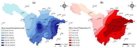
Figure 3.
The spatial patterns in mean annual rainfall (a) and temperature (b) over the UYRB.
4.2. Temporal and Spatial Patterns of Precipitation Variability
4.2.1. Rainfall Trends on Annual and Seasonal Scales
The results of autocorrelation analysis in precipitation series during the period of 1951–2020 are shown in Table A2, along with the Z statistics of the MK/MMK tests. Statistically, there are only two annual series and four seasonal rainfall series that autocorrelate at the 5% significance level. The annual precipitation series of the Yichang and Youyang stations are autocorrelated. The Mianyang and Maduo stations are autocorrelated in winter precipitation, Rongjiang station is autocorrelated in spring precipitation and Chongqing station is autocorrelated in autumn precipitation. Among 34 stations, the annual precipitation series of 22 stations show decreasing trends, with only two significant decreasing trends occurring. The annual series of the other 12 stations show increasing trends, with 4 showing significant increasing trends. On the basis of the seasonal time scale, the number of stations in uptrend is almost the same as the downtrend in the winter, spring and summer scales, accompanied by several significant increases and decreases. However, 23 out of 34 stations show decreasing trends in autumn precipitation, with significant downtrends occurring in two stations at the 5% significant level. The slope magnitudes of rainfall trends over the seven decades are shown in Table A2, with units given in millimeters per decade. The magnitude of statistically long-term trends is determined using Theil–Sen’s slope estimator. The trend slope in annual rainfall varies from −44.67 mm (Yibin station) to 18.00 mm per decade (Chongqing station), with an average magnitude of −3.92 mm per decade over the entire basin. The trend magnitude in winter rainfall is the lowest among the four seasons (0.09 mm per decade in mean), with an increasing trend on the whole. The average slope of precipitation at 34 stations show downtrends in other seasons. In addition, the trend magnitude in autumn precipitation is the highest, with a mean slope of −2.01 mm per decade and a downward trend in general. All stations show non-significant increases in the magnitude of change in autumn precipitation.
The spatial patterns of the trend slope and Hurst exponent in precipitation on annual and seasonal scales are shown in Figure 4. On the annual scale, the spatial pattern verifies the preceding results that most of the basin shows a decreasing trend in rainfall. Rainfall trends in the northern part of the basin appear to be persistent, that is, the changing trend in the future will be the same as the trend in the past. This Hurst phenomenon indicates a decreasing trend similar to the last 70 years in annual rainfall for the area in the future. On the basis of seasonal scales, the winter rainfall exhibited an increasing trend in the southern basin during 1951–2020, while, from the Hurst exponent, an anti-persistent trend occurs in this area. This means that winter rainfall may show a decreasing trend in the southern basin in the future. A persistent trend with a Hurst value around 0.8 appears in the winter rainfall in the northern basin and a slight downtrend during the last seven decades. Hence, winter precipitation in the northern part of the basin may decrease slightly in the future. The spring precipitation in the western part of the basin has an increasing trend, while that in the eastern part has a decreasing trend over the last 70 years. Combined with the spatial distribution maps, summer and autumn rainfall in the middle of the basin (Sichuan Plain) decreased in the past seven decades, and the decreasing trend is likely to continue in the future. The rainfall in Sichuan Plain significantly decreased (at 5% significance level) on all time scales except for winter. Generally, Figure 4 shows a positive magnitude of change (uptrend) in rainfall at higher elevations (Tibet Plateau) and a negative magnitude of change (downtrend) in rainfall at lower elevations (Sichuan Plain), which is in accordance with the discussion of [20].
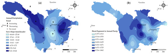

Figure 4.
Spatial distribution of (a) trend magnitude and significance and (b) Hurst exponent in annual and seasonal precipitation over the UYRB during 1951–2020.
4.2.2. Homogeneity Test
Pettitt’s test, SNHT test and Buishand’s test were applied for testing the homogeneity of annual rainfall series. The results of possible change points in annual rainfall are shown in Table A3. The SNHT test tends to find change points towards the beginning and end of the time series, whereas Pettitt’s and Buishand’s tests are sensitive to the changes in the middle of a series [16,19,20]. From the Table A3, it is concluded that most of rainfall series are homogeneous, even though the rainfall of several stations (i.e., Mianyang, Kangding, Yibin, Bijie and Maduo) show heterogeneity. Moreover, all four abrupt change points appear in the 1980s or early 1990s. The homogeneity tests show that four annual rainfall series show heterogeneity around the 1980s, meaning that there is a significant change in the mean before and after the detected change point [20].
4.3. Temporal and Spatial Patterns of Temperature Variability
4.3.1. Temperature Trends on Annual and Seasonal Scales
The results of the autocorrelation analysis for annual and seasonal temperature series are presented in Table A5 along with the Z statistics of the MK/MMK tests during the period from 1951 to 2020. Most of the time series show a lag first-order autocorrelation at a 95% confidence level. Among 34 stations, 33 stations show significant serial correlation on an annual scale, and 13, 17, 19 and 19 stations show significant autocorrelation for winter, spring, summer and autumn seasons, respectively. A majority of the temperature series exhibit an increasing trend on both annual and seasonal scales. For instance, there are 32 annual temperature series showing upward trends, among which 24 series have a significant uptrend at 95% confidence level. Similarly, 33 temperature series (26 significant at 5% level), 33 series (22 at 5% level), 27 series (22 at 5% level) and 30 series (23 at 5% level) show increasing trends in winter, spring, summer and autumn seasons, respectively. During the period of 70 years, only the series of 1 station in winter, 3 stations in summer and 1 station in autumn exhibit a significant decreasing trend. Table A5 further shows the trend slopes in annual and seasonal temperature over the seven decades. The units are calculated in C per decade. The result of Sen’s slope indicates that majority of the stations exhibits upward trends in temperature series on annual and seasonal scales, which is in good accordance with the Z-value of the MK(MMK) test. It should be noticed that the trend magnitude of change in temperature is the most dominant for the winter season, with a mean slope of 0.18 C per decade, which is in line with the analysis of [58]. An average slope of 0.10 C for the summer season is found as the lowest uptrend compared to other seasons. The annual temperature series of the stations in and around the basin increases by an average trend slope of 0.13 C per decade. In general, the estimation of magnitude of the trend slope in temperature series depicts that both annual and seasonal temperatures have been increasing on the basin scale.
On the annual scale, Figure 5 shows significant increasing trends (at 95% confidence interval) in mean temperature for almost the entire basin, except for Guiyang station, over the period of record. On the basis of the seasonal scales, the magnitude of the mean air temperature in the winter, summer and autumn seasons change (increase trend) has decreased from the western part to the eastern part of the whole basin. The highest slope of temperature increases occurred at high altitudes (Tibetan Plateau). In contrast, temperature increases at lower elevations such as the eastern part of the basin were smaller. With the exception of a few stations in the eastern basin, no downward trend in temperature was observed, and significant temperature increases were observed almost throughout the basin. As can be seen from the Hurst exponent charts, the winter mean temperature in the western basin will continue to increase in a high range in the future, with a Hurst value of around 0.75. The trend of the spring mean temperature in the northern and central parts of the basin will continue, that is, the spring temperature in the northern part seems to increase significantly in the future. The mean autumn temperature in the central part of the catchment (Sichuan Plain) will continue the trend of the past 70 years, with the Hurst exponent of about 0.85. Overall, the Hurst value of the mean air temperature is almost in range of 0.50–1, indicating that the temperature in the whole basin may continue to increase significantly in the future, especially in the high altitude area (Qinghai–Tibet Plateau).
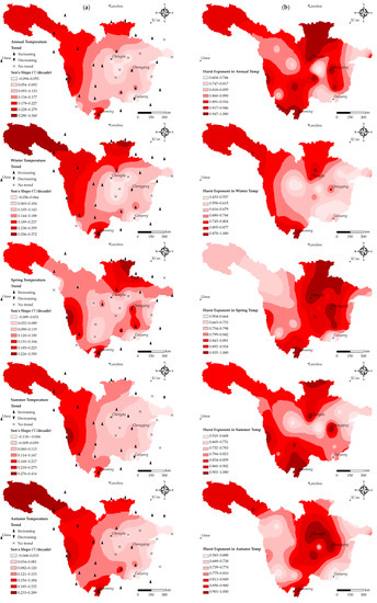
Figure 5.
Spatial distribution of (a) trend magnitude and significance and (b) Hurst exponent in annual and seasonal temperature over the UYRB during 1951–2020.
4.3.2. Homogeneity Test
Pettitt’s test, the SNHT test and Buishand’s test were used to detect the homogeneity of temperature series. Table A5 shows the probable step-change points in annual temperature. Statistical result indicates that majority of series were heterogeneous, with abrupt change points detected in the time series. Among 34 gauging stations, only 3 stations (Neijiang, Youyang and Yunxian) show homogeneity in the annual mean temperature. The homogeneity tests indicate that 20 out of 34 annual temperature series are heterogeneous with abrupt-change around the year 1997, which means a significant change in the mean temperature before and after the change point (1997) [19]. In addition, five stations show heterogeneity with change points around 1993. Hence, the mean annual temperature over the basin changed significantly in the 1990s, with the most probable year being 1997.
4.4. Temporal Variations in Hydroclimatic Variables
4.4.1. Long-Term Pattern on Annual and Seasonal Scales
The time series of watershed rainfall, temperature and runoff on annual and seasonal scales were used to identify the long-term pattern of hydro-climatic factors at different time scales. By means of comparing the long-term patterns (trend and changing time) of the three variables at annual and seasonal time scales, we attempt to initially assess the impact of climate factors (i.e., precipitation and temperature) on streamflow. Since rainfall can only contribute to downstream streamflow [39], the time series of climatic variables were calculated by the spatially averaged value over the basin. The total precipitation and mean temperature series over the basin were calculated by using the Thiessen Polygon method [68] (e.g., [39,58]). While using a weighted average of the data results in a reduction in variance, this reduction is akin to the natural spatial aggregation represented in the runoff [39]. Since the running mean is not resistant to local fluctuations, it is pertinent to reduce local fluctuations by fitting the time series with locally weighted scatterplot smoothing (LOWESS) regression curves [16,19,20]. LOWESS regression curves were fitted over time based on the annual and seasonal series of three variables. It should be noticed that the LOWESS regression lines shown in Figure 6 were used to show patterns over time and did not explain statistically significant trends in the time series [16,20].
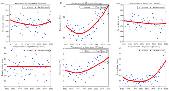
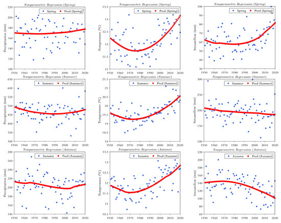
Figure 6.
LOWESS regression line for (a) precipitation, (b) temperature, and (c) streamflow on annual and seasonal scales over the UYRB. Pred means prediction.
The LOWESS regression curves for precipitation, as seen in Figure 6a, indicates decreasing pattern in the rainfall up to 1990 in annual series and an increasing trend thereafter. The LOWESS regression curve for seasonal rainfall in winter depicts no trend and remains almost smooth during the 1951–2020 period. The spring rainfall has shown no obvious trend, increasing slightly throughout the seven decades. From Figure 6a it can be seen that summer rainfall has followed a similar trend to the annual rainfall. This may be related to the dominance of summer precipitation in terms of annual precipitation. The rainfall in autumn indicates a decreasing trend up to 2000, after which it increases gradually.
The LOWESS regression curves of temperature shown in Figure 6b indicate a decreasing trend up to 1972, while a steep increasing trend in mean temperature is evident from 1973 on the annual scale. Figure 6b also shows the LOWESS regression curves for seasonal temperature series depicting similar patterns. A downward trend before the 1970s and a steep upward trend thereafter occur on all time scales. Generally, the LOWESS regression curve based on the annual and seasonal data suggests an increase in temperature over the entire basin during the last 50 years (from the 1970s to 2020).
The LOWESS regression curves of Figure 6c indicate a decreasing pattern of the annual streamflow over the recorded period. The trend starts sharply increasing for the winter and spring seasons in the 1990s and a gradual decreasing pattern in streamflow before then. Moreover, the LOWESS curve indicates a slight downtrend in summer streamflow over the period of 70 years. For the autumn streamflow, a steep downward trend starts in the 1990s, whereas trend increased gradually before then. The observed mode of the summer streamflow is similar to the annual streamflow, since the summer runoff dominates the annual flow.
Variations in the streanflow on a majority of seasonal scales are sharp. Changes in the seasonal precipitation are not sufficient to explain the long-term patterns in the streamflow on the same scale. It has been documented that a substantial increase in air temperature may explain some of the observed increases in winter and spring seasons’ runoff [69]. The upper Yangtze basin has been remarkably affected by human activities, especially in dam construction [57]. This has undoubtedly affected hydrological regimes to an unknown degree. The damming effect on runoff has been a topic of considerable research interest [70]. As reported by [70], the discharge of the Lancang–Mekong River, in the dry season, is obviously lower in the post-dam period than in the pre-dam period, while that in the rainy season is marginally lower in the post-dam period. Rottler et al. [11] has reported that runoff in central European rivers increase in winter and spring and decrease in summer and at the beginning of autumn, but this redistribution of annual flow is mainly attributed to reservoir constructions in the Alpine ridge. Seasonal rainfall over the catchment has almost remained constant in the last seven decades, except for a slight upward trend shown in spring precipitation. However, seasonal streamflow has changed significantly. The different trends in seasonal runoff variations are likely due to the construction and operation of Three Georges Dam (TGD). Construction of the TGD began in 1993 with flow regulation and water impoundment commencing in 2003 [39]. It has been reported that Three Gorges Dam likely mitigated the occurrence of high-flow events at Yichang station located near the dam [39]. As reported by [58], it is possible that storage delays in dams in the Yangtze catchment affect the monthly distribution of discharge. The findings of this study indicate a sharp decreasing trend in autumn (dry season) streamflow and steep increasing trends in winter and spring (rainy season) in the last 20–30 years, which is in accordance with the work of [39,58]. The changes can be explained by operation of hydroelectric and flood control dams [58]. Reservoirs store rainy season streamflows while increasing dry season water supplies and providing a source to supplement of dry season streamflow. Hence, the dam’s regulation appeared to exert a strong influence on trends in streamflow and precipitation-adjusted streamflow on a seasonal scale. Our results confirm the effectiveness of the TGD in providing seasonal flow regulation (for Yichang station) to some degree. In view of this, the operation of the TGD reduced the impacts of floods in spring and summer, while the water stored is released over the winter and autumn seasons to maintain downstream flows for water supply and to facilitate navigation. However, nothing can be detected at the annual scale that indicates a response by the river to the development caused by human activities such as dam construction in the basin. The reason for this may be the context that individual dams in the Yangtze system are small in hydrological terms; the largest is the TGD, yet its storage capacity is only 9% of the mean annual flow of the upper basin [71]. Preceding research found that human activities, especially large dam construction such as the TGD, in the river basin mainly effect the relocation of seasonal runoff and have little influence on annual flow regime [72], which is in accordance with this study.
4.4.2. Change Point Detection
The abrupt-change points in watershed hydroclimatic parameters on annual and seasonal scales were detected by means of Cumulative Sum Charts (CUSUM) analysis. The step change year correspond to the point furthest from 0 in the CUSUM chart, which estimates the last point before the change point occurred [12]. The results of the CUCUM analysis performed for hydroclimatic variables during 1951–2020 are shown in Figure 7. In general, the CUSUM charts of the precipitation series show irregular fluctuations on both the annual and seasonal scales, among which, a change from upward direction to downward direction (decreasing) is shown in the CUSUM chart of annual rainfall during 1951 to 2020. The CUCUM charts of temperature show a change from a downward direction to an upward direction (increasing) on both the annual and seasonal scales. Moreover, the CUSUM charts of streamflow show a variation from an upward direction to a downward direction (decreasing), except for the winter and spring seasons, while an increasing trend in shown in winter and spring streamflows.
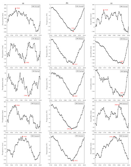
Figure 7.
CUSUM charts of (a) precipitation, (b) temperature and (c) streamflow on annual and seasonal scales over the UYRB during 1951–2020.
As shown in Figure 7, the abrupt change point of each time series was marked by a dot with the change year noted in red. For annual time series, the abrupt-change year of both precipitation and streamflow is shown in 1968. Previous research has reported that the intensity of human activities in the Yangtze River basin has increased dramatically since the reforms and opening of the Chinese economy starting in 1978 [71]. Changes in the annual precipitation and runoff appear to be almost consistent before then. No correlation was observed from the CUSUM analysis between the exploitation dates of dams and the detected trends or the changing points of the annual time series of streamflow. Previous study has indicated that despite the intensive dam building, population growth and economic development in the Yangtze catchment, annual discharge has not been affected in any significant way [58]. The change point of temperature is shown in the year 1997 on all time scales except for the summer season (change in 1993), which coincides with the former analysis. It is worth noting that the change points in both winter and spring streamflows are shown in 2007, and an abrupt change is shown in the year 2000 for the summer season. There have been major programs of dam construction in the Yangtze basin over the period 1955–2014, which do not seem to have affected annual discharge in the Yangtze; yet, it is possible that storage delays in dams affect the monthly distribution of discharge, as reported by [58].
4.4.3. Linear Regression Analysis
Based on the results of the CUSUM analysis, the annual series of three factors were divided to calculate the mean value before and after change years. The annual hydroclimatic series and their linear trends are given in Figure 8. From the linear trend in Figure 8, the time series of precipitation and streamflow exhibit decreasing trends, while a significant increasing trend in air temperature (p < 0.05) is shown with an R value of 0.445 (e.g., [71]). Over the last seven decades, there is an almost consistent variation between rainfall and runoff, especially extreme rainfall years such as the year 1954, which is the highest rainfall and runoff year during the period of 1951 to 2020. Similarly, the year 2006 is both the lowest rainfall and runoff year and the highest year in temperature over the 70-year period. There is a corresponding relationship shown between extreme annual rainfall years and extreme annual runoff years. From the mean values before and after the change year in Figure 8, the magnitude of change in the mean annual precipitation and streamflow seem to be coincide before and after 1968 and both reduce by 30 mm or so. However, the annual mean temperature has an increase of 0.83 C after 1997 compared to before then.
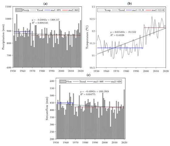
Figure 8.
Time series of annual (a) precipitation, (b) temperature and (c) streamflow and linear trend over the UYRB during 1951–2020. Mu1 denotes mean before mutation; mu2 denotes mean after mutation.
Generally, the increase in temperature promotes the decrease in runoff by speeding up the evaporation of water [3]. The warmer surroundings accelerate evaporation, including the evaporation from open channels of the river, soil, shallow groundwater and water stored in vegetation, and extend the thickness and area of the dried soil layer [45]. Part of the streamflow will return directly to the atmosphere because of evaporation, plant transpiration, dried soil layer and so on, the land surface with depleted water storage can become a larger container to absorb precipitation. It has been reported that temperature increases are generally accompanied by decreases in rainfall in the northern hemisphere [65]. The findings of this study show increasing temperatures and decreasing rainfall and runoff on an annual scale over the UYRB during 1951–2020, indicating a decrease in water availability and the possibility of drought events. The variations in rainfall, temperature and runoff indicate the possibility of the occurrence of drier climate events. These hydrologic changes result from the collective effects of temperature and rainfall variations.
4.5. Sensibility of Streamflow to Climatic Variables
To identify the sensitivity of runoff to climatic factors (precipitation and temperature) at different time scales, the Spearman’s rank correlation test (SRC) was performed for monthly, seasonal and annual time series. The results of the Spearman coefficient between precipitation and streamflow (temperature and streamflow) are shown in Figure 9a,b, among which DJF means winter, MAM means spring, JJA means summer and SON means autumn.
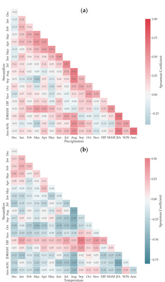
Figure 9.
The Spearman correlation coefficient between (a) precipitation and streamflow and (b) temperature and streamflow at different time scales over the UYRB during 1951–2020.
The correlation is approximately 0.5 for streamflow response to the precipitation of the current month and the previous month. The fluctuation in summer precipitation can explain 68% of summer runoff variability. On the annual scale, the Spearman correlation coefficient between rainfall and runoff is 0.71, indicating that annual precipitation explained 71% of annual runoff. The streamflow variability is found to be strongly related to the rainfall variability over the UYRB, as reported by [39]. The variation in annual runoff is mainly controlled by climate fluctuation (i.e., precipitation variations) in the YRB [72]. Previous research has reported that [71], in multiple correlation analyses of discharge, precipitation, dam volume, population and GDP over the UYRB, only precipitation is significantly correlated with discharge, explaining 80% of the variance. It has been proved that natural drivers (mainly precipitation) can explain runoff variations in the Yangtze catchment, which is the main driver of changes in runoff [71]. Su et al. [39] also stated that the Yangtze basin streamflow is strongly related to rainfall, particularly at coarser (seasonal to annual) timescales. From Figure 9b, a negative correlation between runoff and temperature is shown in most of the time scales, since the increasing temperatures will increase evapotranspiration and decrease runoff [73]. It is worth noting that the temperature in August show a Spearman correlation of −0.51 with August runoff, and the correlation between the summer temperature and autumn streamflow is −0.54. Hence, the temperature in August may have profound effects on the current and the subsequent runoff. However, the correlation between temperature and streamflow is only −0.22 on an annual scale. Increasing temperature corresponds to the gradual decrease in water quantity [14]. It can be expected that temperature increase would lead to more evaporation and transpiration and therefore to less river discharge [58]. The available literature indicated that significant increasing trends in temperature have occurred widely across the UYRB, but there is no indication that the temperature increases have had a detectable impact on runoff, which is in line with the findings of this study [58,71].
5. Conclusions
This paper investigates the long-term variability of hydroclimatic parameters across the UYRB during from 1951 to 2020. The sensitivities of streamflow to climatic factors are tested at the basin scale. The main conclusions are drawn as follows:
- (i).
- The annual rainfall series of 29 out of 34 stations appear homogeneous, while only 3 out of 34 stations are homogeneous in temperature, indicating that 31 series of annual mean temperature have long-term movement during the recorded period, among which the change years (jump points in the mean value) of 20 series occur around the year 1997; that is, the multi-year average value in annual mean temperature has changed thereafter.
- (ii).
- Annual precipitation in the central basin shows a significant decreasing trend, decreasing mainly in summer, while the annual precipitation in the eastern and western parts of the basin show a significant increasing trend. However, for annual and seasonal scales, there are few detectable trends and consistent significant changes in precipitation at most stations. However, mean air temperature shows a significant upward trend on both annual and seasonal scales throughout the basin, except for a minority of sites in the eastern catchment.
- (iii).
- In general, the increasing magnitude in temperature in high altitudes (Tibetan Plateau) is higher than that in low altitudes (Sichuan Plain). The mean air temperature exhibit a Hurst phenomenon on annual and seasonal scales, i.e., the (positive) persistence of temperature. The significant uptrend in high-altitude (such as Tibetan Plateau) temperatures in the future may be comparable with that of the last seven decades in this region.
- (iv).
- The Three Gorges Dam (TGD) provides an effective water-storage and regulation effect on seasonal runoff of Yichang station. Since the TGD was put into operation in 2003, runoff has increased sharply in winter and spring (dry season) and decreased in summer and autumn (rainy season), especially in autumn, while there is no consistent change in precipitation in the basin on the corresponding scale. Hence, the seasonal streamflow variation in the basin can be attributed to high-intensity anthropogenic activities, mainly the intra-annual regulation of the Three Gorges Reservoir (TGR). The TGR releases water during the dry season and stores water during the rainy season to provide water for the dry season.
- (v).
- The watershed precipitation and streamflow from 1951 to 2020 both changed abruptly in 1968, and the mean temperature changed significantly abruptly in 1997 (with a p-value of <0.001 by the Pettitt test). The significant upward trend in annual mean temperature combined with the downward trend in annual precipitation and runoff indicate the amount of available water resources in the basin decreased and the climate tended to be warmer and drier.
- (vi).
- Although the runoff at Yichang station has been strongly impacted by the TGD, the response of annual runoff to dam operation cannot be detected. The annual streamflow is mainly controlled by climatic fluctuation (i.e., variations in precipitation). Changes in post-dam runoff are governed by changing rainfall and dam regulation [39]. The variations in post-dam runoff can be interpreted by considering the probable effects of rainfall variability and dam regulation.
- (vii).
- Runoff in the UYRB is more sensitive to changes in precipitation than changes in temperature. The variation in annual precipitation can explain 71% of annual runoff variability. In contrast, the mean annual temperature has a smaller effect on annual runoff, explaining only −22% of the variability. Overall, runoff is positively correlated with precipitation and negatively correlated with temperature, with increased temperature promoting increased evapotranspiration over the watershed, which leads to a decrease in runoff.
As reported by Zhang et al. [62], the spatial distribution of precipitation and temperature trends is different over the Yangtze basin. In general, the upper Yangtze basin is dominated by a downward precipitation trend and an upward temperature trend. Previous research suggests that the average temperatures are projected to increase in the upper Yangtze basin during the 21st century, and annual rainfall is likely to decrease with the greatest reduction occurring in the summer [59]. In addition, the precipitation variability will be smaller in high-elevation regions, while the fluctuations in temperature in high elevations is expected to be larger than fluctuations in low elevations [59]. As reported by Niu et al. [42], warming extremes were projected to increase while cold events were projected to decrease on the eastern Tibetan Plateau. The above descriptions support a portion of results from this study. The analyses of precipitation trends for this region and of runoff trends for Yichang station indicate that runoff trends respond well to the precipitation trends [62]. As documented by Sun et al. [59], climate change could reduce runoff in the UYRB and exacerbate water supply problems in the region. A decrease in temperature may offset the impact of decreasing rainfall on runoff [72], which means that increasing temperature and decreasing rainfall may intensify the reduction in runoff. As indicated by Xiao et al. [72], the response of runoff to precipitation is more sensitive than that to temperature, with the response to temperature being only one-third of that to precipitation, which is consistent with the findings of this study.
This study provides a vulnerability picture of climate change in the UYRB at annual and seasonal scales, offering important information for future risk decisions and sustainable management of water resources in the basin. The spatial representation of detected precipitation and temperature trends enables a better understanding of climate change in the UYRB over the last 70 years, particularly in terms of spatial patterns of these changes [69]. Reasonable interpretation of these test results require caution. The results of homogeneity tests are generally regarded as the more mundane problems of data quality control. In the absence of a satisfactory explanation of non-homogeneity in the station history, however, the test results should be examined in the context of the broader variations in atmospheric circulation and climate variability [36]. Previous researches revealed that North Atlantic Oscillation (NAO) is the predominantly governing factor affecting climatic parameters, particularly in precipitation patterns [29,36]. There is a strong correlation between precipitation and the NAO index, with precipitation tending to decrease in the positive NAO epochs and increase in the negative NAO epochs [29,74]. It is therefore a high possibility that the NAO could explain a portion of the variance in annual and seasonal rainfall totals, and that its inter-annual variations could result in trend behaviour in rainfall time series [36]. Hence, the change points detected in precipitation records of stations in the UYRB may be attribute to the intensification of the positive phases of NAO, particularly since the 1980s [29]. An important finding of this study is the abrupt increase in the mean temperature over the UYRB at the end of the 1990s. It would be of critical importance to include the issue of trend change in the year 1997 within the new scenarios investigated in the future studies of climate change. It has been documented that the increase in the global temperature is especially evident after 1990s [13,15,33]. The greenhouse gases existed in the atmosphere during the 1990s were greater than at any time during the last half-million years [14]. Moreover, the prolonged positive phase of El Niño Southern Oscillation (ENSO) dominated the 1991–1994 and warmed the global mean surface temperatures, especially in Northern Hemisphere [75]. These may explain the changing trend and abrupt-change behavior of the mean air temperature in the UYRB. Further analysis should be conducted to unequivocally attribute the observed trends to climate change and/or variability. Whether the observed changes are in response to greenhouse gas forcing, or that are part of a natural decadal time scale variation, is a highly controversial issue and difficult to assess, as discussed by Hurrell and van Loon [76]. Whatever the outcome of this debate, the trend features displayed in some of the climatic records could be attribute to changes in atmospheric circulation patterns and should not be removed for the sake of producing homogeneous records [36]. The causes of the different spatial and temporal trends such as increasing atmospheric greenhouse gases or natural climate variability [35] or just a oscillation of multi-interdecadal cycles [16] cannot be adequately explained by a study of this nature. Notwithstanding, the results presented in this study seem to indicate clear past and future trends and pave the way for future hydroclimatic investigations concerning the UYRB.
This paper provides first knowledge on the assessment of possible effects of climate change on the upper Yangtze River. The combined effect of decrease in precipitation and increase in temperature is predicted/expected to contribute to the decrease in streamflow of UYRB. A statistically significant correlation was found between the streamflow and precipitation. The adverse impacts of climate change could be one of the reason for reduction in the amounts of available water resources. However, it is necessary to emphasize the importance of trend analysis of hydrologic variables within a watershed assumed to be free of anthropogenic disturbances. Under certain geomorphic conditions, the nature of river reflects the integrated watershed response to climatic forcing. Since the geomorphologic evolution of a watershed is rather slow compared to climate change, detectable changes in the hydrological regime of a stable, unregulated watershed can be considered as a reflection of climate change [31]. In addition to understanding the effects of climate change on hydrological processes, such analyses may provide independent evidence to confirm and/or validate the results of trend detection for climate variables [25]. With that in mind, future research should directed at the causal aspects of streamflow changes in these environments (undisturbed/natural watersheds). The upper Yangtze River is abundant in hydropower potential, and intensive hydropower development is underway. With the construction of the Three Gorges Dam and other large-scale hydraulic structures on the mainstream and tributaries, river discharge may have been highly disturbed [61]. Changes in surface properties caused by accelerated urbanization after 1980s may have resulted in increased water storage area [71]. Anthropogenic impacts such as the construction of large reservoirs and land use changes hinder the capacity for understanding the possible impacts of climate change on water resource systems [77]. Intensive human activity and watershed surface properties also contribute to the apparent complexity of interpreting changes in runoff. Our results show some connections between streamflow behavior and changes in atmospheric variables, but do not adequately explain the observed runoff variability. What remains unexplained are variations in streamflow due to continuous changes in other watershed attributes (e.g., land use/cover change, natural and anthropogenic changes in river systems, etc.) [78]. We acknowledge the need for further study to more fully understand these results, however it should be recognized that they do contribute to streamflow variability.
Author Contributions
Conceptualization, B.X. and R.Y.; methodology, B.X. and R.Y.; resources and data curation, B.X.; software and visualization, R.Y.; writing—original draft preparation, R.Y.; writing—review and editing, B.X. and R.Y. All authors have read and agreed to the published version of the manuscript.
Funding
This research was funded by the Science and Technology Research Project of Chongqing Municipal Education Commission upon the grant number of KJQN201800711.
Institutional Review Board Statement
Not applicable.
Informed Consent Statement
Not applicable.
Data Availability Statement
The monthly precipitation and temperature time series were obtained from the National Climate Center (NCC) of the China Meteorological Administration (CMA) (http://cmdp.ncc-cma.net/cn/download.htm, accessed on 21 October 2021).
Acknowledgments
The study is financially supported by the Science and Technology Research Project of Chongqing Municipal Education Commission (KJQN201800711). We appreciate the National Climate Center (NCC) of the China Meteorological Administration (CMA) for providing the precipitation and temperature data. The authors wish to thank the anonymous reviewers for their careful review and also for their insightful suggestions and comments that improved the original manuscript to a great extent.
Conflicts of Interest
The authors declare no conflict of interest.
Appendix A. Methodology
Appendix A.1. Autocorrelation Test
The Mann–Kendall test requires tested time series to be serially independent [5]. The existence of serial correlation affects the power of trend tests to identify trends correctly in the time series data [78,79]. Positive serial correlation can overestimate the likelihood of a trend, whereas negative correlation may result in underestimation. Hence, it is essential to evaluate the serial correlation to check randomness and periodicity in a time series prior to conducting trend analysis [5,12]. To this end, the significance of serial correlation was detected in this paper using Student’s t test at lag-1 for rainfall and temperature series, with the formula given below:
where the test statistic t has a Student’s t distribution with () degrees of freedom. If , the null hypothesis about serial independence is rejected at significance level , i.e., significant autocorrelation.
Appendix A.2. Trend Detection
Appendix A.2.1. Mann–Kendall Test
Trend analysis is one of effective tools for detecting changes in hydrologic and climatic series [78]. Numerous parametric and non-parametric tests have been applied for trend detection [80]. Parametric trend tests are more powerful than non-parametric ones, but they require data to be independent and normally distributed [13]. Non-parametric trend tests require only that the data be independent and can tolerate outliers in the data [78,81]. The most common nonparametric test for working with time series trends is the Mann–Kendall (MK) [82,83] test, which is recommended by the World Meteorological Organization (WMO) [84]. The MK test is the rank based non-parametric test which applied by numerous researchers to detect temporal trends and its significant in hydro-climate series [85,86,87].
Test statistic S is defined as:
where and are the annual data values in years j and i, respectively, n is the length of the data, such that , and where the function is given as:
when , the statistic S is approximately normally distributed with the mean and variance as:
where m is the number of tied groups, and denotes size of the th tied group. The standardized test statistic Z is computed using:
The trend results in this study were evaluated at the 5% significant level (the corresponding threshold value is ± 1.96). This implies that the null hypothesis is rejected when in Equation (A4) at level of significance. The alternate hypothesis is that a trend exists in the data. A positive Z value indicates an increasing trend, while a negative Z value indicates a decreasing trend. The significance levels (p-values) for each trend test can be obtained from the relationship given as:
where denotes the cumulative distribution function (CDF) of a standard normal variate. At a significance level of 5%, if , then the existing trend is considered to be statistically significant.
Appendix A.2.2. Modified Mann–Kendall Test
Hydroclimatic series normally display statistically significant serial correlation, which affects the power of trend tests to identify trends correctly in time series data [79,88]. The existence of positive serial correlation increases the probability that the MK test detects a trend when no trend exists. Prewhitening is a procedure for the reduction of serial correlation within a given time series by adding white noise (serially independent) series to the original series. It has been documented that removal of positive serial correlation by prewhitening removes a portion of trend [73], then reduces the detection rate of significant trend in MK test [19,20]. Hence, the Modified Mann–Kendall (MMK) test proposed by Hamed and Rao [78] is employed for trend detection of an autocorrelated series in this study. The calculation process is as follows:
Only significant values of are used to calculate variance correlation factor , as the variance of S is underestimated when data are positively auto-correlated:
where n is the actual number of observations, is considered as an ‘effective’ number of observations to account for autocorrelation in data, and is the autocorrelation function of ranks of the observations. The correlated variance is then computed as:
where
The standardized test statistic is computed by:
where
As confirmed by Hamed and Rao [78], the modification does not influence the power of the MK test, offering more accurate significance levels. However, the MK test is still advocated for detection of trends for time series that do not have significant serial correlation [88].
Appendix A.3. Trend Slope
The Mann–Kendall (MK) test shows the trend existence and trend direction, however, it is not available to show the trend magnitude [18]. For this purpose, the slope of n pairs of data points was estimated using the Theil–Sen’s estimator, as an unbiased median based slope estimator [12], the calculation is given by:
where and are observed values at times j and , respectively. The median of these N values of is Sen’s estimator of slope. If there is only one datum in each time period, then:
where n is the number of time periods. The median of the N estimated slopes is obtained in the usual way, i.e., the N values of are ranked by and:
The reflects direction of trend in the data, while the value indicates steepness of the trend. By obtaining the confidence interval of at specific probability, ones determine whether the median slope is statistically different than zero. The confidence interval about the time slope can be computed as [12]:
where is defined in Equation (A3), and is obtained from the standard normal distribution table.
Appendix A.4. Test for Homogeneity
Appendix A.4.1. Pettitt’s Test
The Pettitt’s test is a nonparametric test that requires no assumption about the distribution of data [79]. The Pettitt’s test is an adaptation of the rank-based Mann–Whitney test that allows identifying the time at which the shift occurs. The null hypothesis H0 indicates that the T variables follow one or more distributions that have the same location parameter, with alternative hypotheses reestablished as below:
Two-tailed test: Ha: There exists a time t from which the variables change location parameters.
Left-tailed test: Ha: There exists a time t from which the variable’s location is reduced by D.
Right-tailed test: Ha: There exists a time t from which the variables location is augmented by D.
The statistic used for the Pettitt’s test is computed as follows:
Let:
The Pettitt’s statistic for the various alternative hypotheses is given by:
Appendix A.4.2. Alexandersson’s SNHT Test
The Standerd Normal Homogeneity Test (SNHT) was developed by Alexandersson [89] and Moberg [90] to detect a change in a series of rainfall data. The test is applied to a series of ratios that compare the observations of a measuring station with the average of several stations [19,20]. The ratios are then standardized. The series of corresponds here to the standardized ratios. The null and alternative hypotheses are determined by:
H0: The T variables follow an distribution.
Ha: Between times 1 and n the variables follow an distribution, and between and T, they follow an distribution.
The statistic is defined by:
with
The statistic derives from a calculation comparing the likelihood of the two alternative models. The model corresponding to Ha implies that and are estimated while determining the n parameter maximizing the likelihood.
Appendix A.4.3. Buishand’s Q Test
The Buishand’s test [91] can be used on variables following any type of distribution. However, its properties have been particularly studied for the normal case. It has been reported that Buishand focuses on the case of the two tailed test, but for the Q statistic presented below, the one-sided cases are also possible [16]. Buishand has developed a second statistic R, for which only a bilateral hypothesis is possible. In the case of the Q statistic, the null and alternative hypotheses are shown as:
H0: The T variables follow one or more distributions that have the same mean.
Two-tailed test: Ha: There exists a time t from which the variables change mean.
Left-tailed test: Ha: There exists a time t from which the variables mean is reduced by .
Right-tailed test: Ha: There exists a time t from which the variables’ mean is augmented by .
Define:
and
The Buishand’s Q statistics are computed ass follows:
The null and alternative hypotheses are given by:
H0: The T variables follow one or more distributions that have the same mean.
Two-sided test: Ha: The T variables are not homogeneous for what concerns their mean.
The Buishand’s R statistic is computed as:
Appendix A.5. R/S Analysis
The rescaled range (R/S) analysis method, one of the widely used non-parametric methods for estimating the Hurst exponent [80], was adopted to estimate future changing trends in hydrological time series. British hydrology expert Hurst firstly proposed an R/S method to establish the Hurst index (H) to describe the continuous state of the hydrological process when studying the hydrological environment of the Nile River. It has been subsequently improved and widely used by several scholars in study of precipitation series [92]. Basic principles and calculation procedures were discussed by Granero et al. [93] in detail. The Hurst exponent H is closely related to the fractal dimension of fractional Brownian motion, which indicates persistence (or anti-persistence) of fractional Brownian motion [72]. The H value is in the range of (0, 1), with its meaning as follows: (1) H (0, 0.5) means that time series has anti-persistence behavior, that is, the general trend of future changes is contrary to the past, and the increase in the past suggests a tendency to decrease in the further; (2) H = 0.5 denotes that the time series are independent of each other, i.e., the value of any time has nothing to do with the past; (3) H (0.5, 1) indicates that the time series has persistent behavior, which means that changing trend in the future will be the same as trend in the past. The smaller the H value, the stronger the reverse anti-persistence, while the greater the H value, the stronger the persistence. The Hurst index (H) can better reveal the trend components in a time series. The calculation of H exponent is given as:
where R is range, S is standard deviation, n is sample size and c is a constant.
Appendix A.6. Kriging Method
The Kriging method that is widely used for spatial interpolation in order to draw zoning maps for trend slope and is a robust geostatistical technique. The trend-magnitude and Hurst index were spatially interpolated by applying the Kriging method after applying and comparing different interpolation methods (e.g., Inverse Distance Weighted, IDW), which is in accordance with Khalili et al. [48]. Applying other interpolation methods can also result in similar output map [44,62,94].
Appendix A.7. Thiessen Polygon Method
The spatial distribution of meteorological stations is highly heterogeneous. The basin rainfall series is the spatially averaged value across 34 gauging stations using the Thiessen Polygon Method, since the approach accounts for heterogeneous distribution of rainfall points, allowing for a more reasonable representation of aggregated rainfall [39]. This method assigns an area called the Thiessen polygon to each station, thereby providing an area-weighted average, which was applied to all stations within a given basin to attain the aggregate basin rainfall [58]. The calculation watershed temperature series follows the same procedure as rainfall.
Appendix A.8. Cumulative Sum Charts
Numerous methods can be used to determinate shifts in the mean and variance of a time series [12]. The Cumulative Sum Charts (CUSUM) test [79] was applied in detecting the abrupt-change points in hydroclimatic series in this study. The changing trend can also be visually determine through the curve. When the cumulative anomaly curve is on the rise, it indicates the increase in anomaly, namely, the upward trend; otherwise, it indicates the downward trend [72]. For a given time series , the cumulative anomaly at a moment t is expressed as:
where , is the cumulative anomaly from year 1 to year t, is the sample value of year i, and is the mean value of sample data. The CUSUM chart follows a relatively straight line, signifying a period when the average did not change, while an abrupt change in the direction of CUSUM indicates an abrupt shift in the average. The point m means the last point before the change point occurred [12].
Appendix A.9. Spearman’s Rank Correlation Coefficient Test
The Spearman s rank correlation coefficient (SRC) test [95] is a rank-based test for correlation between two variables [84] that can also be used to test for measuring the strength of a monotonic relationship between the time and data series [54]. As an extensively used nonparametric test, the power of this test is comparable with the MK test [79]. For two given time series , the Spearman coefficient is calculated as:
where . is the rank of the variable , is the chronological order of observations and in series of size n. The test statistic is given by Equation (A28):
Test statistic follows a t-distribution with the degree of freedom and significance level . The null hypothesis of no trend is rejected when . statistic is approximately normally distributed for the statistic [81].
Appendix B

Table A1.
Meteoroligical gauging stations with its code used for this study.
Table A1.
Meteoroligical gauging stations with its code used for this study.
| Number | Station | Code | WMO Number | Latitude (°N) | Longitude (°E) |
|---|---|---|---|---|---|
| 1 | Yushu | YUS | 56029 | 33.02 | 97.02 |
| 2 | Ganzi | GAN | 56146 | 31.62 | 100 |
| 3 | Mianyang | MAY | 56196 | 31.47 | 104.68 |
| 4 | Ya’an | YAN | 56287 | 29.98 | 103 |
| 5 | Chengdu | CHE | 56294 | 30.67 | 104.02 |
| 6 | Kangding | KAN | 56374 | 30.05 | 101.97 |
| 7 | Yibin | YIB | 56492 | 28.8 | 104.6 |
| 8 | Xichang | XIC | 56571 | 27.9 | 102.27 |
| 9 | Lijiang | LIJ | 56651 | 26.83 | 100.47 |
| 10 | Huili | HUI | 56671 | 26.65 | 102.25 |
| 11 | Kunming | KUN | 56778 | 25.02 | 102.68 |
| 12 | Daxian | DAX | 57328 | 31.2 | 107.5 |
| 13 | Nanchong | NAN | 57411 | 30.8 | 106.08 |
| 14 | Enshi | ENS | 57447 | 30.28 | 109.47 |
| 15 | Yichang | YIC | 57461 | 30.7 | 111.3 |
| 16 | Neijiang | NEI | 57504 | 29.58 | 105.05 |
| 17 | Chongqing | CHO | 57516 | 29.52 | 106.48 |
| 18 | Youyang | YOU | 57633 | 28.83 | 108.77 |
| 19 | Bijie | BIJ | 57707 | 27.3 | 105.23 |
| 20 | Zunyi | ZUN | 57713 | 27.7 | 106.88 |
| 21 | Guiyang | GUI | 57816 | 26.58 | 106.72 |
| 22 | Maduo | MAD | 56033 | 34.92 | 98.22 |
| 23 | Minxian | MIN | 56093 | 34.43 | 104.01 |
| 24 | Changdu | CHA | 56137 | 31.15 | 97.17 |
| 25 | Deqin | DEQ | 56444 | 28.5 | 98.9 |
| 26 | Dali | DAL | 56751 | 25.7 | 100.18 |
| 27 | Tianshui | TAS | 57006 | 34.58 | 105.75 |
| 28 | Hanzhong | HAN | 57127 | 33.07 | 107.03 |
| 29 | Ankang | ANK | 57245 | 32.72 | 109.03 |
| 30 | Zhijiang | ZHI | 57745 | 27.45 | 109.68 |
| 31 | Xingren | XIN | 57902 | 25.43 | 105.18 |
| 32 | Lahsa | LAS | 55591 | 29.67 | 91.13 |
| 33 | Rongjiang | RON | 57932 | 25.97 | 108.53 |
| 34 | Yunxian | YUN | 57253 | 32.51 | 110.49 |
Table A2.
Results of MK/MMK test (at 5% level) and trend slope in annual and seasonal rainfall over the UYRB during 1951–2020. Bold indicates passing the 5% significance level. The italics represent the MMK values of precipitation series with autocorrelation. Positive/negative Z value indicates increasing/decreasing trend.
| Station | Annual | Winter | Spring | Summer | Autumn | |||||
|---|---|---|---|---|---|---|---|---|---|---|
| Z | Slope | Z | Slope | Z | Slope | Z | Slope | Z | Slope | |
| YUS | 1.04 | 5.45 | 0.10 | 0.00 | 3.15 | 4.00 | −0.41 | −2.07 | 1.82 | 2.41 |
| GAN | 2.33 | 11.90 | 0.38 | 0.18 | 1.35 | 3.75 | 1.24 | 5.45 | 0.40 | 1.05 |
| MAY | −2.00 | −29.21 | −0.23 | 0.00 | −1.77 | −3.79 | −2.15 | −26.67 | −0.98 | −4.44 |
| YAN | −1.83 | −30.00 | 0.36 | 0.40 | 0.02 | 0.00 | −0.69 | −12.29 | −5.04 | −10.88 |
| CHE | −0.69 | −8.75 | 0.53 | 0.43 | −1.31 | −3.64 | −0.51 | −4.21 | −0.24 | −0.95 |
| KAN | 5.39 | 16.47 | −0.10 | 0.00 | 1.95 | 6.79 | 1.72 | 7.41 | 0.49 | 1.67 |
| YIB | −2.98 | −44.67 | −1.90 | −1.89 | −4.10 | −11.76 | −1.88 | −20.48 | −1.29 | −6.18 |
| XIC | 0.14 | 1.61 | −0.64 | −0.36 | 1.18 | 4.80 | 0.09 | 1.11 | −1.54 | −6.59 |
| LIJ | −0.25 | −1.88 | 1.23 | 0.33 | 1.17 | 3.53 | −1.03 | −7.02 | 0.27 | 1.67 |
| HUI | −0.43 | −5.67 | 0.93 | 0.54 | 1.86 | 6.49 | −1.17 | −10.00 | −0.85 | −4.80 |
| KUN | −0.45 | −2.80 | 4.64 | 2.67 | 0.14 | 0.71 | −0.55 | −3.72 | nan | −3.53 |
| DAX | 0.66 | 9.60 | −0.01 | 0.00 | 1.00 | 4.55 | 1.19 | 11.03 | −0.23 | −2.13 |
| NAN | 0.34 | 3.70 | −0.48 | −0.39 | 0.11 | 0.50 | 0.82 | 8.48 | −0.96 | −5.22 |
| ENS | −0.01 | −0.17 | −0.61 | −0.48 | −0.72 | −4.50 | 0.13 | 1.76 | −0.15 | −1.67 |
| YIC | −1.10 | −8.37 | 0.05 | 0.00 | −1.79 | −6.44 | −0.64 | −8.44 | 1.02 | 3.33 |
| NEI | −1.19 | −18.15 | −1.45 | −1.00 | 0.48 | 1.61 | nan | −6.47 | −1.97 | −5.64 |
| CHO | 2.55 | 18.00 | 0.05 | 0.00 | 1.05 | 5.56 | 1.24 | 10.48 | 0.07 | 0.50 |
| YOU | −0.15 | −2.59 | 0.83 | 1.18 | −0.79 | −4.74 | 0.44 | 4.40 | −0.58 | −2.94 |
| BIJ | −1.86 | −17.50 | −2.16 | −1.85 | −1.75 | −5.17 | −0.66 | −4.00 | −0.92 | −3.83 |
| ZUN | −0.90 | −8.26 | 0.08 | 0.00 | −1.75 | −8.33 | 1.04 | 7.71 | −1.01 | −5.79 |
| GUI | −0.46 | −6.11 | 0.72 | 1.07 | −1.42 | −8.89 | 0.32 | 3.03 | −0.60 | −2.92 |
| MAD | 2.75 | 11.67 | 0.80 | 0.36 | 3.52 | 3.85 | 2.04 | 5.33 | 1.79 | 2.38 |
| MIN | 0.17 | 1.25 | −0.53 | 0.00 | −0.38 | −0.74 | 0.46 | 1.77 | −0.22 | −0.43 |
| CHA | −0.05 | −0.47 | −0.27 | 0.00 | 1.28 | 2.08 | −0.93 | −3.44 | 1.65 | 3.49 |
| DEQ | −1.44 | −10.81 | −1.85 | −1.61 | 0.69 | 2.33 | −1.67 | −6.50 | −0.47 | −1.52 |
| DAL | −1.14 | −15.08 | 1.35 | 2.63 | 1.02 | 4.69 | −1.33 | −8.51 | −1.18 | −7.65 |
| TAS | −0.95 | −5.24 | −0.26 | 0.00 | 0.74 | 1.86 | −0.75 | −4.07 | −1.35 | −4.00 |
| HAN | −1.31 | −13.25 | −1.72 | −1.16 | −0.25 | −0.86 | −0.76 | −7.00 | −0.11 | −0.94 |
| ANK | 0.85 | 7.42 | −0.37 | −0.25 | −1.32 | −4.17 | 2.17 | 8.97 | −0.25 | −1.82 |
| ZHI | −0.10 | −0.86 | 0.70 | 2.25 | −2.50 | −16.73 | 1.69 | 17.12 | −0.23 | −1.43 |
| XIN | −0.88 | −8.57 | −0.09 | 0.00 | −2.43 | −13.75 | 0.94 | 7.21 | −1.10 | −4.55 |
| LAS | 0.98 | 5.29 | 0.84 | 0.00 | 3.00 | 2.55 | −0.10 | −0.89 | 0.35 | 0.70 |
| RON | 1.54 | 16.67 | 1.43 | 2.26 | 0.30 | 0.98 | 2.59 | 13.67 | 1.03 | 5.38 |
| YUN | −0.41 | −4.00 | −3.32 | −2.34 | −1.19 | −4.92 | 0.28 | 1.90 | −0.20 | −1.11 |
Table A3.
Most probable change year by Pettitt’s, SNHT and Buishand’s tests for annual rainfall series. Ho denotes Homogeneous series, Ha denotes Heterogeneous series. Ha–Heterogeneous series, Ho–Homogeneous series (in italics).
Table A3.
Most probable change year by Pettitt’s, SNHT and Buishand’s tests for annual rainfall series. Ho denotes Homogeneous series, Ha denotes Heterogeneous series. Ha–Heterogeneous series, Ho–Homogeneous series (in italics).
| Station | Pettitt’s Test | SNHT | Buishand’s Q Test | ||||||
|---|---|---|---|---|---|---|---|---|---|
| K Value | Year | Trend | To Value | Year | Trend | Q Value | Year | Trend | |
| YUS | 256 | 2007 | Ho | 5.13 | 2016 | Ho | 0.82 | 2007 | Ho |
| GAN | 336 | 2010 | Ho | 9.65 | 2011 | Ha | 1.09 | 2010 | Ho |
| MAY | 479 | 1984 | Ha | 10.09 | 1961 | Ha | 1.40 | 1984 | Ha |
| YAN | 325 | 1992 | Ho | 4.88 | 1961 | Ho | 0.95 | 1992 | Ho |
| CHE | 368 | 1967 | Ho | 7.64 | 2012 | Ho | 1.10 | 1967 | Ho |
| KAN | 559 | 1983 | Ha | 11.00 | 1983 | Ha | 1.67 | 1983 | Ha |
| YIB | 547 | 1991 | Ha | 8.98 | 1991 | Ha | 1.49 | 1991 | Ha |
| XIC | 249 | 1959 | Ho | 4.07 | 1957 | Ho | 0.66 | 1959 | Ho |
| LIJ | 292 | 2004 | Ho | 4.21 | 2004 | Ho | 0.87 | 2004 | Ho |
| HUI | 225 | 2005 | Ho | 1.98 | 2005 | Ho | 0.58 | 2005 | Ho |
| KUN | 193 | 1976 | Ho | 1.41 | 2001 | Ho | 0.53 | 1986 | Ho |
| DAX | 217 | 1962 | Ho | 2.78 | 1962 | Ho | 0.67 | 1972 | Ho |
| NAN | 220 | 2006 | Ho | 4.60 | 1952 | Ho | 0.71 | 1975 | Ho |
| ENS | 223 | 1961 | Ho | 2.75 | 2019 | Ho | 0.57 | 1961 | Ho |
| YIC | 148 | 1970 | Ho | 6.58 | 2019 | Ho | 0.39 | 1965 | Ho |
| NEI | 313 | 1991 | Ho | 4.39 | 1991 | Ho | 1.04 | 1991 | Ho |
| CHO | 304 | 2013 | Ho | 7.86 | 2013 | Ho | 0.90 | 1995 | Ho |
| YOU | 171 | 1977 | Ho | 5.10 | 2019 | Ho | 0.54 | 1983 | Ho |
| BIJ | 482 | 1984 | Ha | 10.63 | 1957 | Ha | 1.39 | 1983 | Ha |
| ZUN | 327 | 2002 | Ho | 3.31 | 2004 | Ho | 0.80 | 2002 | Ho |
| GUI | 230 | 2013 | Ho | 4.62 | 1954 | Ho | 0.78 | 1977 | Ho |
| MAD | 585 | 1988 | Ha | 10.71 | 2004 | Ha | 1.55 | 1988 | Ha |
| MIN | 276 | 2011 | Ho | 9.24 | 2017 | Ha | 0.89 | 2011 | Ho |
| CHA | 316 | 1986 | Ho | 3.41 | 1986 | Ho | 0.93 | 1986 | Ho |
| DEQ | 268 | 1966 | Ho | 3.94 | 2010 | Ho | 0.71 | 1966 | Ho |
| DAL | 297 | 2002 | Ho | 5.12 | 2009 | Ho | 0.87 | 2002 | Ho |
| TAS | 317 | 1990 | Ho | 3.19 | 1968 | Ho | 0.79 | 1990 | Ho |
| HAN | 364 | 1990 | Ho | 4.78 | 1984 | Ho | 1.10 | 1984 | Ho |
| ANK | 277 | 2002 | Ho | 3.63 | 2002 | Ho | 0.84 | 2002 | Ho |
| ZHI | 234 | 1972 | Ho | 4.61 | 2019 | Ho | 0.77 | 1972 | Ho |
| XIN | 314 | 1997 | Ho | 4.64 | 2008 | Ho | 0.92 | 1997 | Ho |
| LAS | 380 | 1997 | Ho | 3.55 | 1997 | Ho | 0.89 | 1997 | Ho |
| RON | 310 | 2014 | Ho | 11.80 | 2014 | Ha | 0.97 | 2014 | Ho |
| YUN | 210 | 1990 | Ho | 1.25 | 1964 | Ho | 0.55 | 1990 | Ho |
Table A4.
Results of MK/MMK test (at 5% level) and trend slope in annual and seasonal temperature over the UYRB during 1951–2020. Bold indicates passing the 5% significance level. The italics represent the MMK values of temperature series with autocorrelation. Positive/negative Z value indicates increasing/decreasing trend.
| Station | Annual | Winter | Spring | Summer | Autumn | |||||
|---|---|---|---|---|---|---|---|---|---|---|
| Z | Slope | Z | Slope | Z | Slope | Z | Slope | Z | Slope | |
| YUS | 5.22 | 0.22 | 3.75 | 0.29 | 3.06 | 0.13 | 5.52 | 0.25 | 4.41 | 0.25 |
| GAN | 3.60 | 0.21 | 4.39 | 0.28 | 2.56 | 0.12 | 4.26 | 0.21 | 2.59 | 0.16 |
| MAY | 2.49 | 0.15 | 3.24 | 0.20 | 2.51 | 0.20 | 2.19 | 0.11 | 3.30 | 0.13 |
| YAN | 3.44 | 0.10 | 2.19 | 0.12 | 2.65 | 0.14 | 2.09 | 0.07 | 3.84 | 0.11 |
| CHE | 0.96 | 0.04 | 0.98 | 0.05 | 0.95 | 0.07 | 0.38 | 0.01 | 1.73 | 0.08 |
| KAN | 3.96 | 0.12 | 2.98 | 0.17 | 1.18 | 0.07 | 3.32 | 0.12 | 4.25 | 0.16 |
| YIB | 1.07 | 0.05 | 0.10 | 0.00 | 1.16 | 0.10 | 1.30 | 0.05 | 1.87 | 0.08 |
| XIC | 3.08 | 0.10 | 2.15 | 0.14 | 0.88 | 0.04 | 3.32 | 0.11 | 3.12 | 0.14 |
| LIJ | 5.02 | 0.17 | 4.78 | 0.22 | 3.73 | 0.19 | 5.06 | 0.17 | 3.23 | 0.13 |
| HUI | 1.98 | 0.10 | 3.89 | 0.15 | 0.16 | 0.02 | 2.32 | 0.09 | 2.31 | 0.12 |
| KUN | 3.96 | 0.27 | 3.69 | 0.33 | 3.14 | 0.25 | 4.83 | 0.23 | 4.07 | 0.27 |
| DAX | 1.90 | 0.07 | 2.48 | 0.11 | 2.28 | 0.11 | 0.52 | 0.03 | 1.59 | 0.06 |
| NAN | 0.20 | 0.01 | 0.57 | 0.02 | 0.97 | 0.05 | −0.43 | −0.02 | 0.24 | 0.01 |
| ENS | 1.99 | 0.08 | 2.42 | 0.12 | 2.57 | 0.11 | 0.37 | 0.02 | 1.29 | 0.05 |
| YIC | 1.24 | 0.04 | 1.65 | 0.07 | 3.08 | 0.14 | −1.36 | −0.07 | −0.28 | −0.01 |
| NEI | 0.83 | 0.02 | 0.40 | 0.02 | 0.73 | 0.04 | −0.08 | 0.00 | 1.95 | 0.05 |
| CHO | 2.85 | 0.14 | 2.88 | 0.15 | 2.68 | 0.18 | 2.24 | 0.11 | 2.76 | 0.12 |
| YOU | 0.09 | 0.00 | 0.84 | 0.04 | 0.67 | 0.03 | −1.26 | −0.06 | −0.51 | −0.03 |
| BIJ | 4.45 | 0.14 | 2.78 | 0.17 | 2.40 | 0.16 | 2.97 | 0.11 | 3.77 | 0.17 |
| ZUN | 5.44 | 0.15 | 3.46 | 0.18 | 3.85 | 0.21 | 2.94 | 0.11 | 4.74 | 0.14 |
| GUI | −2.26 | −0.09 | −0.99 | −0.06 | −1.66 | −0.09 | −2.87 | −0.12 | −1.79 | −0.07 |
| MAD | 5.62 | 0.29 | 4.63 | 0.39 | 3.98 | 0.15 | 4.81 | 0.24 | 4.50 | 0.31 |
| MIN | 3.86 | 0.22 | 5.06 | 0.30 | 2.66 | 0.17 | 3.10 | 0.18 | 3.37 | 0.19 |
| CHA | 3.41 | 0.14 | 4.31 | 0.22 | 1.10 | 0.05 | 3.13 | 0.14 | 2.21 | 0.11 |
| DEQ | 7.13 | 0.37 | 5.33 | 0.31 | 5.63 | 0.36 | 5.21 | 0.42 | 5.36 | 0.29 |
| DAL | 1.74 | 0.08 | 0.70 | 0.05 | 1.69 | 0.11 | 2.18 | 0.09 | 2.87 | 0.10 |
| TAS | 4.65 | 0.26 | 5.61 | 0.40 | 3.99 | 0.29 | 3.16 | 0.18 | 4.76 | 0.21 |
| HAN | 4.01 | 0.22 | 5.63 | 0.26 | 3.92 | 0.32 | 2.12 | 0.11 | 4.38 | 0.18 |
| ANK | 2.59 | 0.10 | 3.95 | 0.18 | 2.82 | 0.18 | −1.08 | −0.05 | 3.04 | 0.09 |
| ZHI | 4.66 | 0.12 | 4.35 | 0.19 | 4.13 | 0.18 | 0.48 | 0.02 | 1.96 | 0.09 |
| XIN | 3.20 | 0.15 | 2.59 | 0.18 | 2.03 | 0.14 | 4.55 | 0.13 | 3.83 | 0.18 |
| LAS | 5.54 | 0.38 | 6.52 | 0.47 | 3.95 | 0.25 | 6.81 | 0.33 | 6.47 | 0.41 |
| RON | 3.99 | 0.14 | 2.73 | 0.18 | 3.52 | 0.16 | 3.38 | 0.12 | 5.12 | 0.15 |
| YUN | −0.57 | −0.03 | 2.76 | 0.06 | 1.75 | 0.12 | −3.37 | −0.20 | −2.10 | −0.10 |
Table A5.
Most probable change year by Pettitt’s, SNHT and Buishand’s tests for annual temperature series. Ho denotes Homogeneous series, Ha denotes Heterogeneous series. Ha–Heterogeneous series, Ho–Homogeneous series (in italics).
Table A5.
Most probable change year by Pettitt’s, SNHT and Buishand’s tests for annual temperature series. Ho denotes Homogeneous series, Ha denotes Heterogeneous series. Ha–Heterogeneous series, Ho–Homogeneous series (in italics).
| Station | Pettitt’s Test | SNHT | Buishand’s Q Test | ||||||
|---|---|---|---|---|---|---|---|---|---|
| K Value | Year | Trend | To Value | Year | Trend | Q Value | Year | Trend | |
| YUS | 900 | 1986 | Ha | 31.33 | 1997 | Ha | 2.65 | 1997 | Ha |
| GAN | 832 | 1997 | Ha | 30.43 | 2002 | Ha | 2.46 | 1997 | Ha |
| MAY | 988 | 1993 | Ha | 36.70 | 1996 | Ha | 2.93 | 1993 | Ha |
| YAN | 832 | 1996 | Ha | 27.59 | 1996 | Ha | 2.51 | 1996 | Ha |
| CHE | 710 | 1993 | Ha | 19.77 | 1993 | Ha | 2.18 | 1993 | Ha |
| KAN | 819 | 1997 | Ha | 29.01 | 1997 | Ha | 2.55 | 1997 | Ha |
| YIB | 651 | 1997 | Ha | 18.90 | 1997 | Ha | 2.06 | 1997 | Ha |
| XIC | 714 | 1997 | Ha | 22.13 | 2001 | Ha | 2.13 | 2000 | Ha |
| LIJ | 885 | 1993 | Ha | 35.74 | 2004 | Ha | 2.80 | 1997 | Ha |
| HUI | 730 | 2004 | Ha | 29.16 | 2008 | Ha | 2.27 | 2004 | Ha |
| KUN | 1134 | 1992 | Ha | 48.12 | 1993 | Ha | 3.40 | 1993 | Ha |
| DAX | 748 | 1997 | Ha | 27.40 | 2012 | Ha | 2.28 | 1997 | Ha |
| NAN | 441 | 1996 | Ha | 9.61 | 2005 | Ha | 1.48 | 1996 | Ha |
| ENS | 648 | 1997 | Ha | 26.39 | 2012 | Ha | 2.07 | 1997 | Ha |
| YIC | 503 | 1996 | Ha | 12.69 | 1996 | Ha | 1.70 | 1996 | Ha |
| NEI | 434 | 1997 | Ho | 8.45 | 1997 | Ho | 1.37 | 1997 | Ha |
| CHO | 905 | 1996 | Ha | 31.49 | 1997 | Ha | 2.67 | 1996 | Ha |
| YOU | 383 | 2011 | Ho | 12.79 | 2011 | Ha | 1.21 | 2011 | Ho |
| BIJ | 889 | 1997 | Ha | 32.80 | 1997 | Ha | 2.71 | 1997 | Ha |
| ZUN | 942 | 1997 | Ha | 37.30 | 1997 | Ha | 2.89 | 1997 | Ha |
| GUI | 629 | 1999 | Ha | 15.70 | 1999 | Ha | 1.83 | 1999 | Ha |
| MAD | 1023 | 1997 | Ha | 38.34 | 1997 | Ha | 2.93 | 1997 | Ha |
| MIN | 1018 | 1996 | Ha | 40.52 | 1997 | Ha | 3.03 | 1996 | Ha |
| CHA | 816 | 1997 | Ha | 30.07 | 2004 | Ha | 2.40 | 1997 | Ha |
| DEQ | 1059 | 1993 | Ha | 41.94 | 1993 | Ha | 3.18 | 1993 | Ha |
| DAL | 662 | 1997 | Ha | 23.08 | 2004 | Ha | 2.05 | 2002 | Ha |
| TAS | 1123 | 1993 | Ha | 47.95 | 1993 | Ha | 3.40 | 1993 | Ha |
| HAN | 1074 | 1996 | Ha | 48.19 | 1996 | Ha | 3.32 | 1996 | Ha |
| ANK | 800 | 1996 | Ha | 23.98 | 1996 | Ha | 2.34 | 1996 | Ha |
| ZHI | 881 | 1997 | Ha | 30.86 | 1997 | Ha | 2.63 | 1997 | Ha |
| XIN | 805 | 1997 | Ha | 27.41 | 1997 | Ha | 2.48 | 1997 | Ha |
| LAS | 1105 | 1992 | Ha | 48.07 | 1997 | Ha | 3.32 | 1992 | Ha |
| RON | 986 | 1997 | Ha | 41.62 | 1997 | Ha | 3.05 | 1997 | Ha |
| YUN | 407 | 1979 | Ho | 8.11 | 2012 | Ho | 1.37 | 1979 | Ha |
References
- Caloiero, T. Analysis of rainfall trend in New Zealand. Environ. Earth Sci. 2015, 73, 6297–6310. [Google Scholar] [CrossRef]
- IPCC Working Group I Contribution to the IPCC Fifth Assessment Report, Climate Change 2013: The Physical Science Basis: Summary for Policymakers. Available online: http://www.cmcc.it/wp-content/uploads/2012/12/lista-autori-wgi-ar5.pdf (accessed on 27 January 2021).
- Chen, J.; Gao, C.; Zeng, X.; Xiong, M.; Wang, Y.; Jing, C.; Krysanova, V.; Huang, J.; Zhao, N.; Su, B. Assessing changes of river discharge under global warming of 1.5 °C and 2 °C in the upper reaches of the Yangtze River Basin: Approach by using multiple-GCMs and hydrological models. Quat. Int. 2017, 453, 63–73. [Google Scholar] [CrossRef]
- Chen, Y.; Takeuchi, K.; Xu, C.; Chen, Y.; Xu, Z. Regional climate change and its effects on river runoff in the Tarim Basin, China. Hydrol. Process. 2006, 20, 2207–2216. [Google Scholar] [CrossRef]
- Yue, S.; Hashino, M. Long term trends of annual and monthly precipitation in japan. J. Am. Water Resour. Assoc. 2003, 39, 587–596. [Google Scholar] [CrossRef]
- Arnell, N. Climate change and global water resources. Glob. Environ. Change 1999, 9, S31–S49. [Google Scholar] [CrossRef]
- Shen, Z.; Zhang, Q.; Singh, V.; Sun, P.; Song, C.; Yu, H. Agricultural drought monitoring across Inner Mongolia, China: Model development, spatiotemporal patterns and impacts. J. Hydrol. 2019, 571, 793–804. [Google Scholar] [CrossRef]
- Yang, Y.; Weng, B.; Man, Z.; Yu, Z.; Zhao, J. Analyzing the contributions of climate change and human activities on runoff in the Northeast Tibet Plateau. J. Hydrol. Reg. Stud. 2020, 27, 100639. [Google Scholar] [CrossRef]
- Zhao, Y.; Dong, N.; Wang, H. Quantifying the climate and human impacts on the hydrology of the Yalong River Basin using two approaches. River Res. Appl. 2021, 37, 591–604. [Google Scholar] [CrossRef]
- Miller, W.; Piechota, T.; Gangopadhyay, S.; Pruitt, T. Development of streamflow projections under changing climate conditions over Colorado River basin headwaters. Hydrol. Earth Syst. Sci. 2011, 15, 2145–2164. [Google Scholar] [CrossRef] [Green Version]
- Rottler, E.; Francke, T.; Bürger, G.; Bronstert, A. Long-term changes in central European river discharge for 1869–2016: Impact of changing snow covers, reservoir constructions and an intensified hydrological cycle. Hydrol. Earth Syst. Sci. 2020, 24, 1721–1740. [Google Scholar] [CrossRef] [Green Version]
- Okafor, G.; Jimoh, O.; Larbi, I. Detecting Changes in Hydro-Climatic Variables during the Last Four Decades (1975-2014) on Downstream Kaduna River Catchment, Nigeria. Atmos. Clim. Sci. 2017, 7, 161–175. [Google Scholar] [CrossRef] [Green Version]
- Zhao, G.; Hörmann, G.; Fohrer, N.; Zhang, Z.; Zhai, J. Streamflow Trends and Climate Variability Impacts in Poyang Lake Basin, China. Water Resour. Manag. 2010, 24, 689–706. [Google Scholar] [CrossRef]
- Dogan, M.; Ulke, A.; Cigizoglu, H. Trend direction changes of Turkish temperature series in the first half of 1990s. Theor. Appl. Climatol. 2015, 121, 23–39. [Google Scholar] [CrossRef]
- Novotny, E.; Stefan, H. Stream flow in Minnesota: Indicator of climate change. J. Hydrol. 2007, 334, 319–333. [Google Scholar] [CrossRef]
- Adeyeri, O.; Lamptey, B.; Lawin, A.; Sanda, I. Spatio-Temporal Precipitation Trend and Homogeneity Analysis in Komadugu-Yobe Basin, Lake Chad Region. J. Climatol. Weather. Forecast. 2017, 5, 1000214. [Google Scholar] [CrossRef]
- Xu, J.; Chen, Y.; Ji, M.; Lu, F. Climate change and its effects on runoff of Kaidu River, Xinjiang, China: A multiple time-scale analysis. Chin. Geogr. Sci. 2008, 18, 331–339. [Google Scholar] [CrossRef]
- Salehi, S.; Dehghani, M.; Mortazavi, S.; Singh, V. Trend analysis and change point detection of seasonal and annual precipitation in Iran. Int. J. Climatol. 2020, 40, 308–323. [Google Scholar] [CrossRef]
- Taxak, A.; Murumkar, A.; Arya, D. Long term spatial and temporal rainfall trends and homogeneity analysis in Wainganga basin, Central India. Weather. Clim. Extrem. 2014, 4, 50–61. [Google Scholar] [CrossRef] [Green Version]
- Akinsanola, A.; Ogunjobi, K. Recent homogeneity analysis and long-term spatio-temporal rainfall trends in Nigeria. Theor. Appl. Climatol. 2017, 128, 275–289. [Google Scholar] [CrossRef]
- Ologunorisa, T.; Durowoju, O.; Akinbobola, A. Hydroclimatology of the Kaduna River Basin. Am. J. Clim. Change 2021, 10, 353–369. [Google Scholar] [CrossRef]
- Koutsoyiannis, D. Climate Change, the Hurst Phenomenon, and Hydrological Statistics. Hydrolog. Sci. J. 2003, 48, 3–24. [Google Scholar] [CrossRef]
- Ray, L.; Goel, N. Spatio-temporal change in rainfall over five different climatic regions of India. J. Water Clim. Chang. 2021, 12, 3124–3142. [Google Scholar] [CrossRef]
- Dabanlı, İ.; Şen, Z.; Yeleğen, M.; Şişman, E.; Selek, B.; Güçlü, Y. Trend Assessment by the Innovative-Şen Method. Water Resour. Manag. 2016, 30, 5193–5203. [Google Scholar] [CrossRef]
- Zhang, X.; Harvey, K.; Hogg, W.; Yuzyk, T. Trends in Canadian streamflow. Water Resour. Res. 2001, 37, 987–998. [Google Scholar] [CrossRef]
- Milly, P.; Betancourt, J.; Falkenmark, M.; Hirsch, R.; Kundzewicz, Z.; Lettenmaier, D.; Stouffer, R. Stationarity Is Dead: Whither Water Management? Science 2008, 319, 573–574. [Google Scholar] [CrossRef] [PubMed]
- Chen, H.; Guo, S.; Xu, C.; Singh, V. Historical temporal trends of hydro-climatic variables and runoff response to climate variability and their relevance in water resource management in the Hanjiang basin. J. Hydrol. 2007, 344, 171–184. [Google Scholar] [CrossRef]
- Şen, Z. Innovative Trend Analysis Methodology. J. Hydrol. Eng. 2012, 17, 1042–1046. [Google Scholar] [CrossRef]
- Kukul Kurttaş, Y.; Anaç, S.; Yeşilırmak, E.; de Moraes, J. Trends of precipitation and stream-flow in Gediz river basin, Western Turkey. Fresenius Environ. Bull. 2007, 16, 477–488. [Google Scholar]
- Wu, Z.; Huang, N.; Long, S.; Peng, C. On the trend, detrending, and variability of nonlinear and nonstationary time series. Proc. Natl. Acad. Sci. USA 2007, 104, 14889–14894. [Google Scholar] [CrossRef] [Green Version]
- Kahya, E.; Kalayc, S. Trend analysis of streamflow in Turkey. J. Hydrol. 2004, 289, 128–144. [Google Scholar] [CrossRef]
- Tuomenvirta, Heikki Homogeneity testing and adjustment of climatic time series in Finland. Geophysicsa 2002, 38, 15–41.
- Su, B.; Jiang, T.; Jin, W. Recent trends in observed temperature and precipitation extremes in the Yangtze River basin, China. Theor. Appl. Climatol. 2006, 83, 139–151. [Google Scholar] [CrossRef]
- Falarz, M.; Wibig, J.; Matuszko, D.; Filipiak, J.; Hajto, M.; Taszarek, M.; Bielec-Bąkowska, Z.; Wypych, A.; Ustrnul, Z. Homogeneity of Climate Series. In Climate Change in Poland, Springer Climate; Springer: Berlin/Heidelberg, Germany, 2021. [Google Scholar] [CrossRef]
- Zhang, X.; Vincent, L.; Hogg, W.; Niitsoo, A. Temperature and Precipitation Trends in Canada During the 20th Century. Atmosphere-ocean 2000, 38, 395–429. [Google Scholar] [CrossRef]
- Hall, M. The interpretation of non-homogeneous hydrometeorological time series: A case study. Meteorol. Appl. 2003, 10, 61–67. [Google Scholar] [CrossRef]
- Zhang, Q.; Liu, C.; Xu, C.; Xu, Y.; Jiang, T. Observed trends of annual maximum water level and streamflow during past 130 years in the Yangtze River basin, China. J. Hydrol. 2006, 324, 255–265. [Google Scholar] [CrossRef]
- Tu, M. Assessment of the effects of climate variability and land use change on the hydrology of the Meuse River Basin. In Hydrology and Geo-Environmental Sciences; A.A. Balkema Publishers: Avereest, The Netherlands, 2006. [Google Scholar]
- Su, Z.; Ho, M.; Hao, Z.; Lall, U.; Sun, X.; Chen, X.; Yan, L. The impact of the Three Gorges Dam on summer streamflow in the Yangtze River Basin. Hydrol. Process. 2020, 34, 705–717. [Google Scholar] [CrossRef]
- Shi, G.; Ye, P. Assessment on Temporal and Spatial Variation Analysis of Extreme Temperature Indices: A Case Study of the Yangtze River Basin. Int. J. Environ. Res. Public Health 2021, 18, 10936. [Google Scholar] [CrossRef]
- Yuan, Z.; Yin, J.; Wei, M.; Yuan, Y. Spatio-Temporal Variations in the Temperature and Precipitation Extremes in Yangtze River Basin, China during 1961–2020. Atmosphere 2021, 12, 1423. [Google Scholar] [CrossRef]
- Niu, Z.; Feng, L.; Chen, X.; Yi, X. Evaluation and Future Projection of Extreme Climate Events in the Yellow River Basin and Yangtze River Basin in China Using Ensembled CMIP5 Models Data. Int. J. Environ. Res. Public Health 2021, 18, 6029. [Google Scholar] [CrossRef]
- IPCC. Climate change 2013: The physical science basis. In Contribution of Working Group I to the Fifth Assessment Report of the Intergovernmental Panel on Climate Change; Stocker, T.F., Qin, D., Plattner, G.-K., Tignor, M., Allen, S.K., Boschung, J., Nauels, A., Xia, Y., Bex, V., Midgley, P.M., Eds.; Cambridge University Press: Cambridge, UK; New York, NY, USA, 2013. [Google Scholar]
- Cannarozzo, M.; Noto, L.; Viola, F. Spatial distribution of rainfall trends in Sicily (1921–2000). Phys. Chem. Earth 2006, 31, 1201–1211. [Google Scholar] [CrossRef]
- He, B.; Miao, C.; Shi, W. Trend, abrupt change, and periodicity of streamflow in the mainstream of Yellow River. Environ. Monit. Assess. 2013, 185, 6187–6199. [Google Scholar] [CrossRef]
- Tongal, H. Spatiotemporal analysis of precipitation and extreme indices in the Antalya Basin, Turkey. Theor. Appl. Climatol. 2019, 138, 1735–1754. [Google Scholar] [CrossRef]
- Wang, J.; Wang, K.; Qin, T.; Nie, H.; Lv, Z.; Liu, F.; Shi, X.; Hu, Y. Analysis and prediction of LUCC change in Huang-Huai-Hai river basin. Open Geosci. 2020, 12, 1406–1420. [Google Scholar] [CrossRef]
- Khalili, K.; Tahoudi, M.; Mirabbasi, R.; Ahmadi, F. Investigation of spatial and temporal variability of precipitation in Iran over the last half century. Stoch. Environ. Res. Risk Assess. 2016, 30, 1205–1221. [Google Scholar] [CrossRef]
- Zhang, Q.; Xu, C.; Tao, H.; Jiang, T.; Chen, Y. Climate changes and their impacts on water resources in the arid regions: A case study of the Tarim River basin, China. Stoch. Environ. Res. Risk Assess. 2010, 24, 349–358. [Google Scholar] [CrossRef]
- Proutsos, N.; Tigkas, D. Growth Response of Endemic Black Pine Trees to Meteorological Variations and Drought Episodes in a Mediterranean Region. Atmosphere 2020, 11, 554. [Google Scholar] [CrossRef]
- Fang, L.; Wang, L.; Chen, W.; Sun, J.; Cao, Q.; Wang, S.; Wang, L. Identifying the impacts of natural and human factors on ecosystem service in the Yangtze and Yellow River Basins. J. Clean. Prod. 2021, 314, 127995. [Google Scholar] [CrossRef]
- Yue, S.; Wang, C. A study of variability of annual river flow of the southern African region. Hydrol. Sci. J. 2002, 47, 983–987. [Google Scholar] [CrossRef]
- Fu, G.; Charles, S.; Viney, N.; Chen, S.; Wu, J. Impacts of climate variability on stream-flow in the Yellow River. Hydrol. Process. 2007, 21, 3431–3439. [Google Scholar] [CrossRef]
- Kundzewicz, Z.; Robson, A. Change detection in hydrological records—A review of the methodology. Hydrolog. Sci. J. 2004, 49, 7–19. [Google Scholar] [CrossRef]
- von Storch, H. Misuses of statistical analysis in climate research. In Analysis of Climate Variability; Springer: Berlin/Heidelberg, Germany, 1999; pp. 11–26. [Google Scholar]
- Fang, Y.; Zhang, X.; Niu, G.; Zeng, W.; Zhu, J.; Zhang, T. Study of the Spatiotemporal Characteristics of Meltwater Contribution to the Total Runoff in the Upper Changjiang River Basin. Water 2017, 9, 165. [Google Scholar] [CrossRef] [Green Version]
- Zhang, X.; Liu, P.; Cheng, L.; Xie, K.; Han, D.; Zhou, L. The temporal variations in runoff-generation parameters of the Xinanjiang model due to human activities: A case study in the upper Yangtze River Basin, China. J. Hydrol. Reg. Stud. 2021, 37, 100910. [Google Scholar] [CrossRef]
- Chen, J.; Finlayson, B.; Wei, T.; Sun, Q.; Webber, M.; Li, M.; Chen, Z. Changes in monthly flows in the Yangtze River, China—With special reference to the Three Gorges Dam. J. Hydrol. 2016, 536, 293–301. [Google Scholar] [CrossRef]
- Sun, J.; Tian, Y.; Liao, W.; Wang, Y. Hydrological impacts of climate change in the upper reaches of the Yangtze River Basin. Quat. Int. 2013, 304, 62–74. [Google Scholar] [CrossRef]
- Yang, X.; Yu, X.; Wang, Y.; Liu, Y.; Zhang, M.; Ren, L.; Yuan, F.; Jiang, S. Estimating the response of hydrological regimes to future projections of precipitation and temperature over the upper Yangtze River. Atmos. Res. 2019, 230, 104627. [Google Scholar] [CrossRef]
- Xu, J.; Yang, D.; Yi, Y.; Lei, Z.; Chen, J.; Yang, W. Spatial and temporal variation of runoff in the Yangtze River Basin during the past 40 years. Quat. Int. 2008, 186, 32–42. [Google Scholar] [CrossRef]
- Zhang, Q.; Tong, J.; Gemmer, M.; Becker, S. Precipitation, temperature and runoff analysis from 1950 to 2002 in the Yangtze basin, China. Hydrolog. Sci. J. 2005, 50, 65–80. [Google Scholar] [CrossRef] [Green Version]
- Hu, M.; Dong, M.; Tian, X.; Wang, L.; Jiang, Y. Trends in Different Grades of Precipitation over the Yangtze River Basin from 1960 to 2017. Atmosphere 2021, 12, 413. [Google Scholar] [CrossRef]
- Wei, X.; Cai, S.; Ni, P.; Zhan, W. Impacts of climate change and human activities on the water discharge and sediment load of the Pearl River, southern China. Sci. Rep. 2020, 10, 16743. [Google Scholar] [CrossRef]
- Solaimani, K.; Habaibnejad, M.; Pirnia, A. Temporal trends of hydro-climatic variables and their relevance in water resource management. Int. J. Sediment Res. 2021, 36, 63–75. [Google Scholar] [CrossRef]
- Peterson, T.; Easterling, D.; Karl, T.; Groisman, P.; Nicholls, N.; Plummer, N.; Torok, S.; Auer, I.; Boehm, R.; Gullett, D.; et al. Homogeneity adjustments of in situ atmospheric climate data: A review. Int. J. Climatol. 1998, 18, 1493–1517. [Google Scholar] [CrossRef]
- Huang, Y.; Xiao, W.; Hou, B.; Zhou, Y.; Hou, G.; Yi, L.; Cui, H. Hydrological projections in the upper reaches of the Yangtze River Basin from 2020 to 2050. Sci. Rep. 2021, 11, 9720. [Google Scholar] [CrossRef] [PubMed]
- Thilessen, A. Precipitation Averages for Large Areas. Mon. Weather. Rev. 1911, 39, 1082–1089. [Google Scholar] [CrossRef]
- Birsan, M.; Molnar, P.; Burlando, P.; Pfaundler, M. Streamflow trends in Switzerland. J. Hydrol. 2005, 314, 312–329. [Google Scholar] [CrossRef]
- Wang, Y.; Lei, X.; Wen, X.; Fang, G.; Tan, Q.; Tian, Y.; Wang, C.; Wang, H. Effects of damming and climatic change on the eco-hydrological system: A case study in the Yalong River, southwest China. Ecol. Indic. 2019, 105, 663–674. [Google Scholar] [CrossRef]
- Chen, J.; Wu, X.; Finlayson, B.; Webber, M.; Wei, T.; Mao, T.; Chen, Z. Variability and trend in the hydrology of the Yangtze River, China: Annual precipitation and runoff. J. Hydrol. 2014, 513, 403–412. [Google Scholar] [CrossRef]
- Xiao, Z.; Shi, P.; Jiang, P.; Hu, J.; Qu, S.; Chen, X.; Chen, Y.; Dai, Y.; Wang, J. The Spatiotemporal Variations of Runoff in the Yangtze River Basin under Climate Change. Adv. Meteorol. 2018, 2018, 5903451. [Google Scholar] [CrossRef] [Green Version]
- Asarian, J.; Walker, J. Long-Term Trends in Streamflow and Precipitation in Northwest California and Southwest Oregon, 1953–2012. J. Am. Water Resour. Assoc. 2016, 52, 241–261. [Google Scholar] [CrossRef]
- Tsiros, I.; Nastos, P.; Proutsos, N.; Tsaousidis, A. Variability of the aridity index and related drought parameters in Greece using climatological data over the last century (1900–1997). Atmos. Res. 2020, 240, 104914. [Google Scholar] [CrossRef]
- World Meteorological Organization. Statement on the Status of the Global Climate in 1997; WMO-No.877; WMO: Geneva, Switzerland, 1997. [Google Scholar]
- Hurrell, J.; van Loon, H. Decadal variations in climate associated with the North Atlantic Oscillation. Clim. Change 1997, 36, 301–326. [Google Scholar] [CrossRef]
- Burn, D. Climatic influences on streamflow timing in the headwaters of the Mackenzie River Basin. J. Hydrol. 2008, 352, 225–238. [Google Scholar] [CrossRef]
- Hamed, K.; Rao, A. A modified Mann-Kendall trend test for autocorrelated data. J. Hydrol. 1998, 204, 182–196. [Google Scholar] [CrossRef]
- Patakamuri, S.; Muthiah, K.; Sridhar, V. Long-Term Homogeneity, Trend, and Change-Point Analysis of Rainfall in the Arid District of Ananthapuramu, Andhra Pradesh State, India. Water 2020, 12, 211. [Google Scholar] [CrossRef] [Green Version]
- Li, Z.; Xu, Z.; Li, J.; li, Z. Shift trend and step changes for runoff time series in the Shiyang River basin, northwest China. Hydrol. Process. 2008, 22, 4639–4646. [Google Scholar] [CrossRef]
- Fathian, F.; Morid, S.; Kahya, E. Identification of trends in hydrological and climatic variables in Urmia Lake basin, Iran. Theor. Appl. Climatol. 2015, 119, 443–464. [Google Scholar] [CrossRef]
- Mann, H. Nonparametric Tests Against Trend. Econometrica 1945, 13, 245–259. [Google Scholar] [CrossRef]
- Kendall, M. Rank Correlation Methods; Griffin; American Psychological Association: Washington, DC, USA, 1948. [Google Scholar]
- Sönmez, A.; Kale, S. Climate change effects on annual streamflow of Filyos River (Turkey). J. Water Clim. Chang. 2020, 11, 420–433. [Google Scholar] [CrossRef]
- Kisi, O.; Santos, C.; da Silva, R.; Zounemat-Kermani, M. Trend analysis of monthly streamflows using Sen’s innovative trend method. Geofizika 2018, 35, 53–68. [Google Scholar] [CrossRef]
- Fu, G.; Chen, S.; Liu, C.; Shepard, D. Hydro-Climatic Trends of the Yellow River Basin for the Last 50 Years. Hydrolog. Sci. J. 2004, 65, 149–178. [Google Scholar] [CrossRef] [Green Version]
- Gebremicael, T.; Mohamed, Y.; Zaag, P.; Hagos, E. Temporal and spatial changes of rainfall and streamflow in the Upper Tekeze–Atbara River Basin, Ethiopia. Hydrol. Earth Syst. Sci. 2017, 21, 2127–2142. [Google Scholar] [CrossRef] [Green Version]
- Yue, S.; Pilon, P.; Phinney, B.; Cavadias, G. The influence of autocorrelation on the ability to detect trend in hydrological series. Hydrol. Process. 2002, 16, 1807–1829. [Google Scholar] [CrossRef]
- Alexandersson, H. A homogeneity test applied to precipitation data. J. Climatol. 1986, 6, 661–675. [Google Scholar] [CrossRef]
- Alexandersson, H.; Moberg, A. Homogenization of Swedish Temperature Data. Part i: Homogeneity Test for Linear Trends. Int. J. Climatol. 1997, 17, 25–34. [Google Scholar] [CrossRef]
- Buishand, T. Some methods for testing the homogeneity of rainfall records. J. Hydrol. 1982, 58, 11–27. [Google Scholar] [CrossRef]
- Wu, S.; Hu, Z.; Wang, Z.; Cao, S.; Yang, Y.; Qu, X.; Zhao, W. Spatiotemporal variations in extreme precipitation on the middle and lower reaches of the Yangtze River Basin (1970–2018). Quat. Int. 2021, 592, 80–96. [Google Scholar] [CrossRef]
- Sánchez-Granero, M.; Trinidad Segovia, J.; García Pérez, J. Some comments on Hurst exponent and the long memory processes on capital markets. Phys. A Stat. Mech. Appl. 2008, 387, 5543–5551. [Google Scholar] [CrossRef]
- Gumus, V. Spatio-temporal precipitation and temperature trend analysis of the Seyhan–Ceyhan River Basins, Turkey. Meteorol Appl. 2019, 26, 369–384. [Google Scholar] [CrossRef] [Green Version]
- Spearman, C. The proof and measurement of association between two things. Int. J. Epidemiol. 2010, 39, 1137–1150. [Google Scholar] [CrossRef] [Green Version]
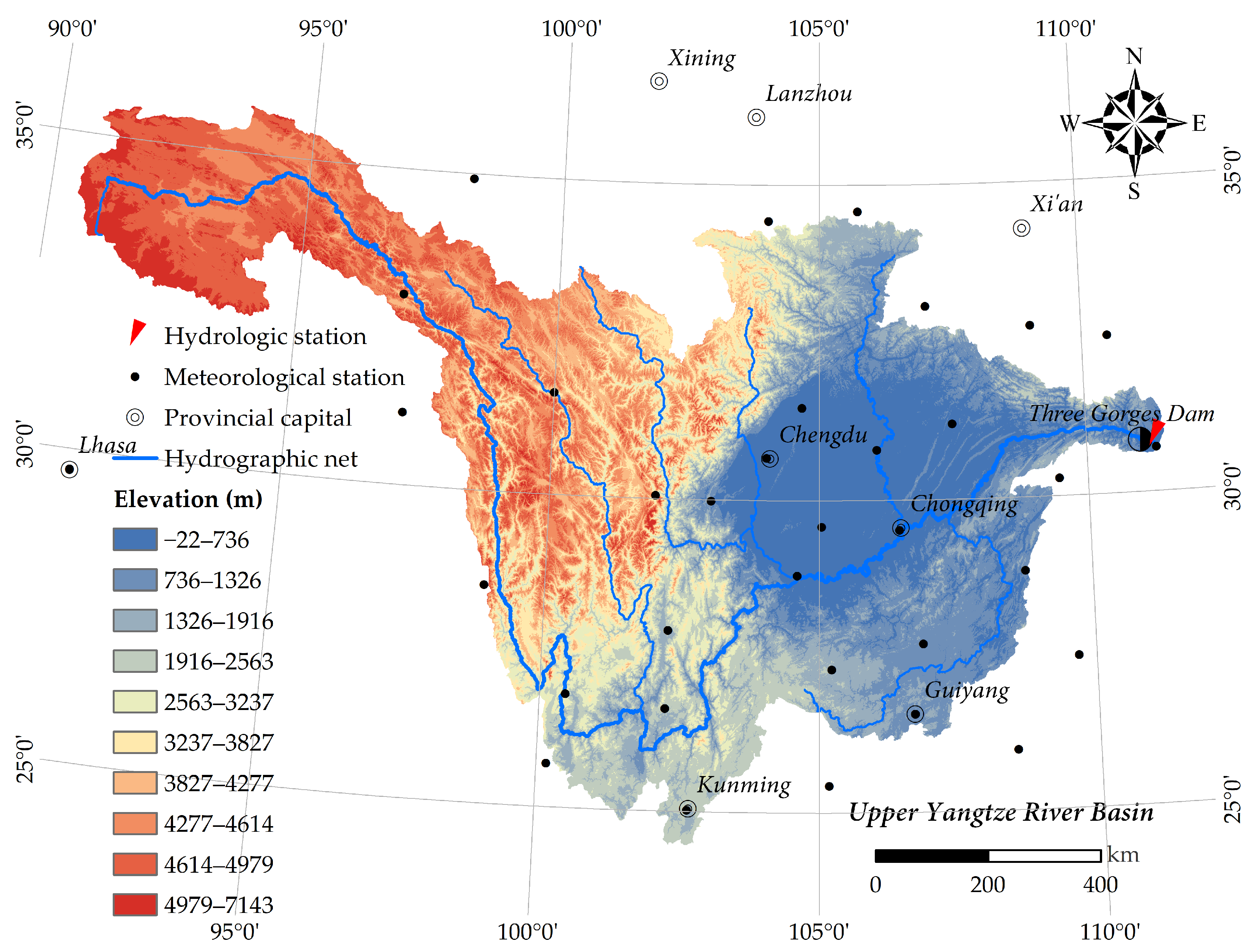
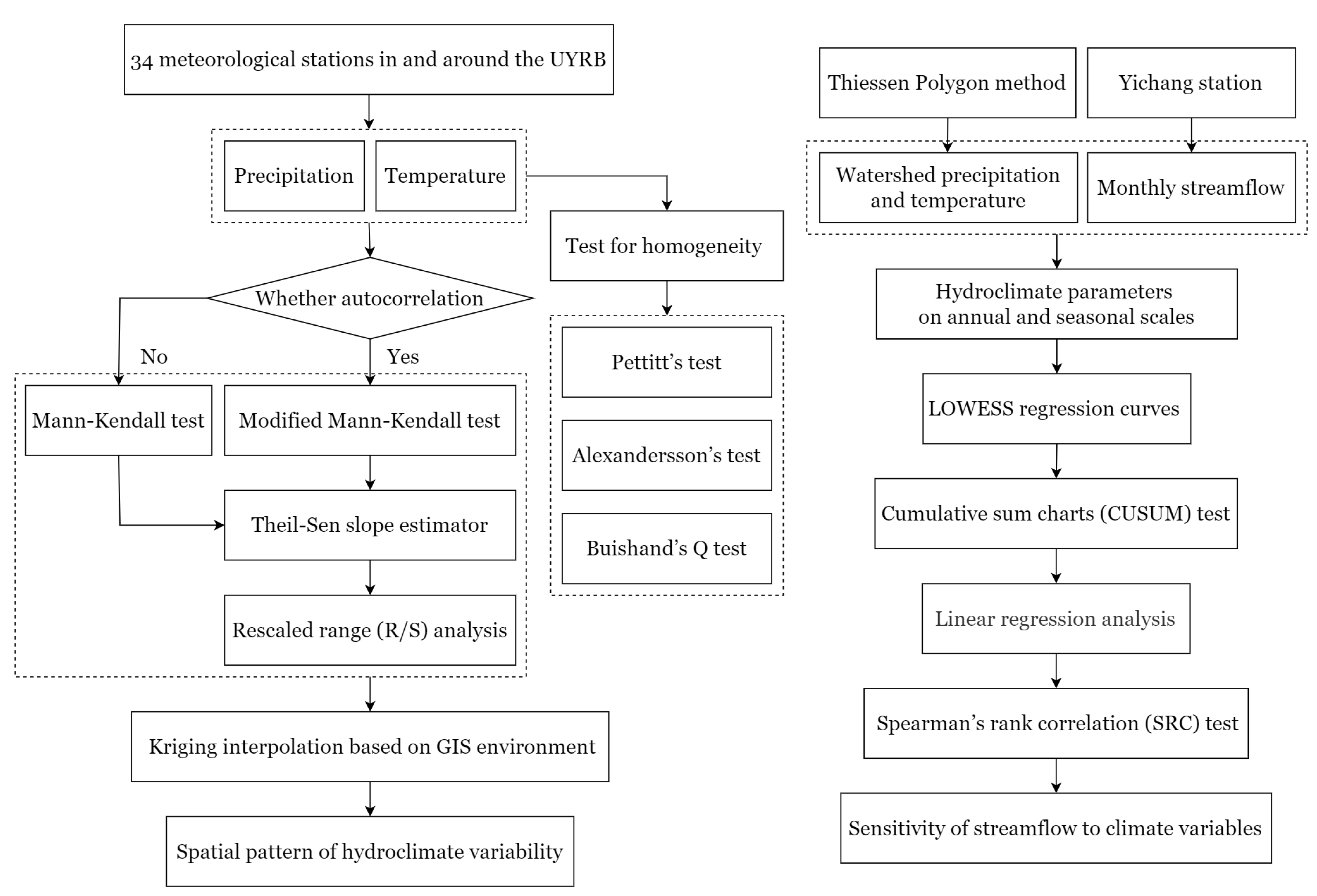
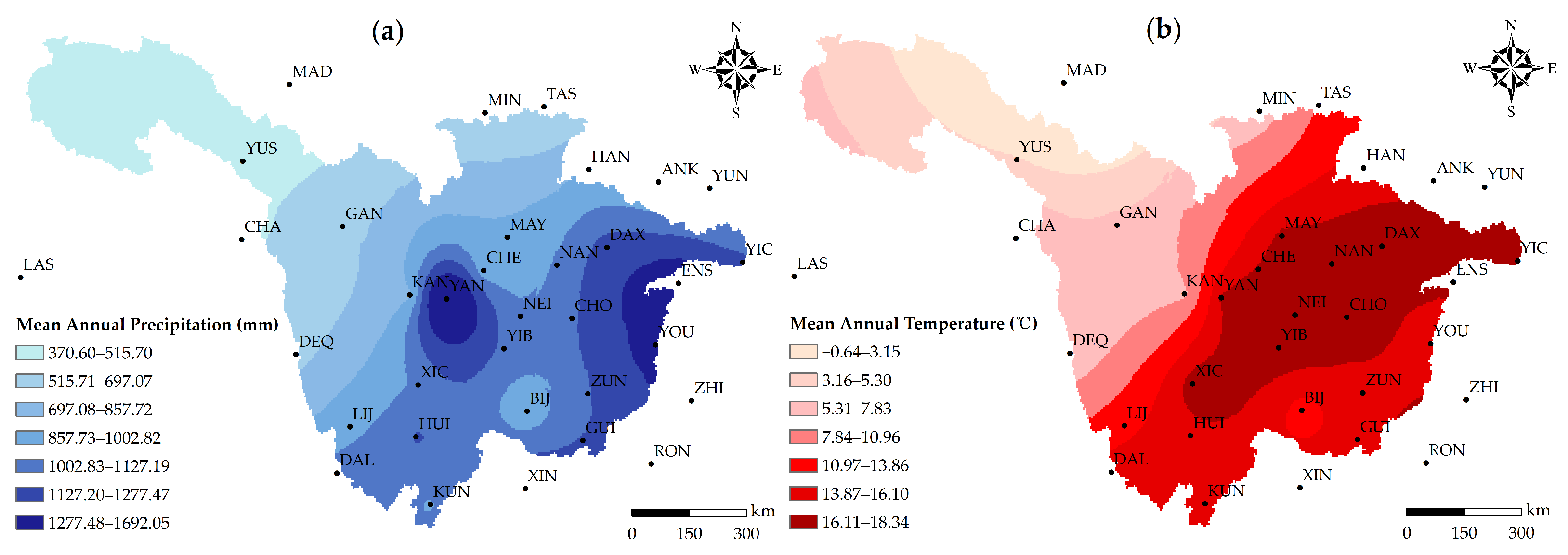
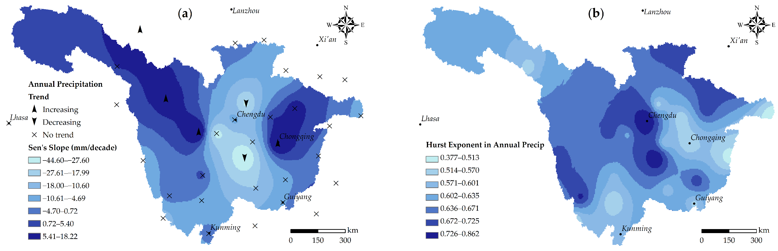
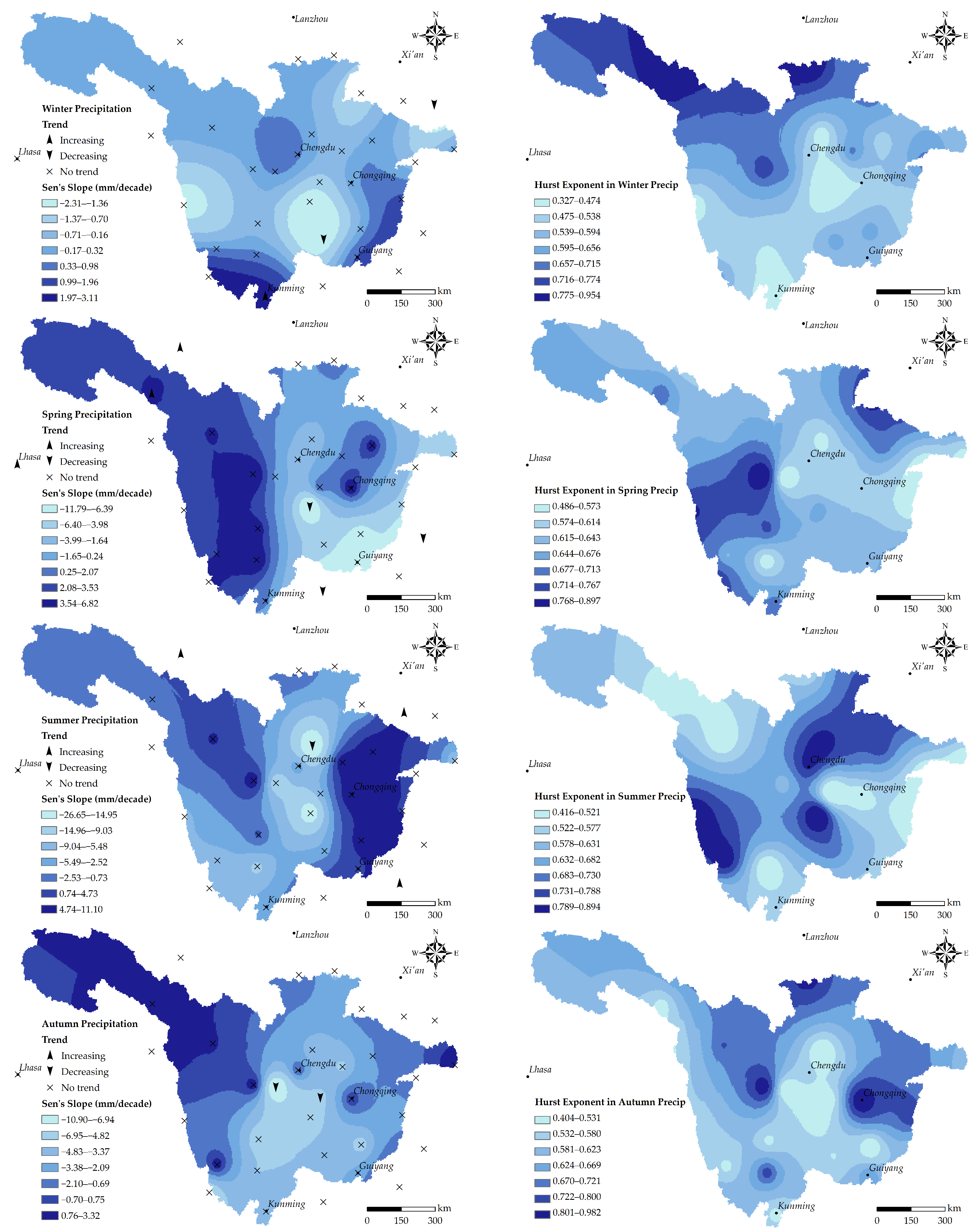


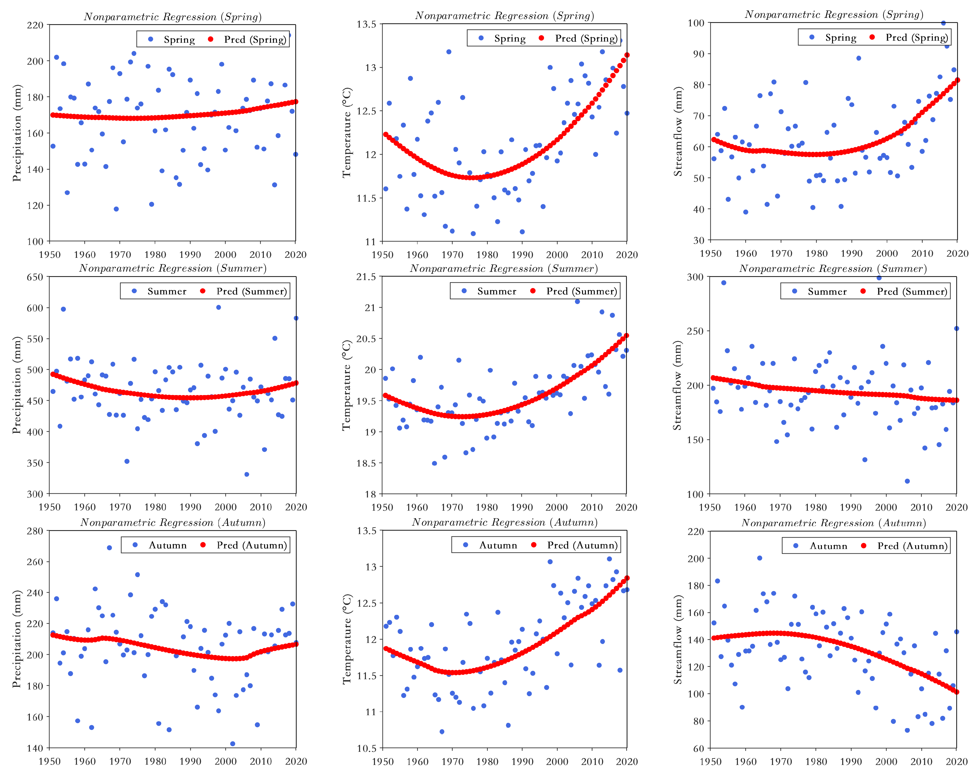
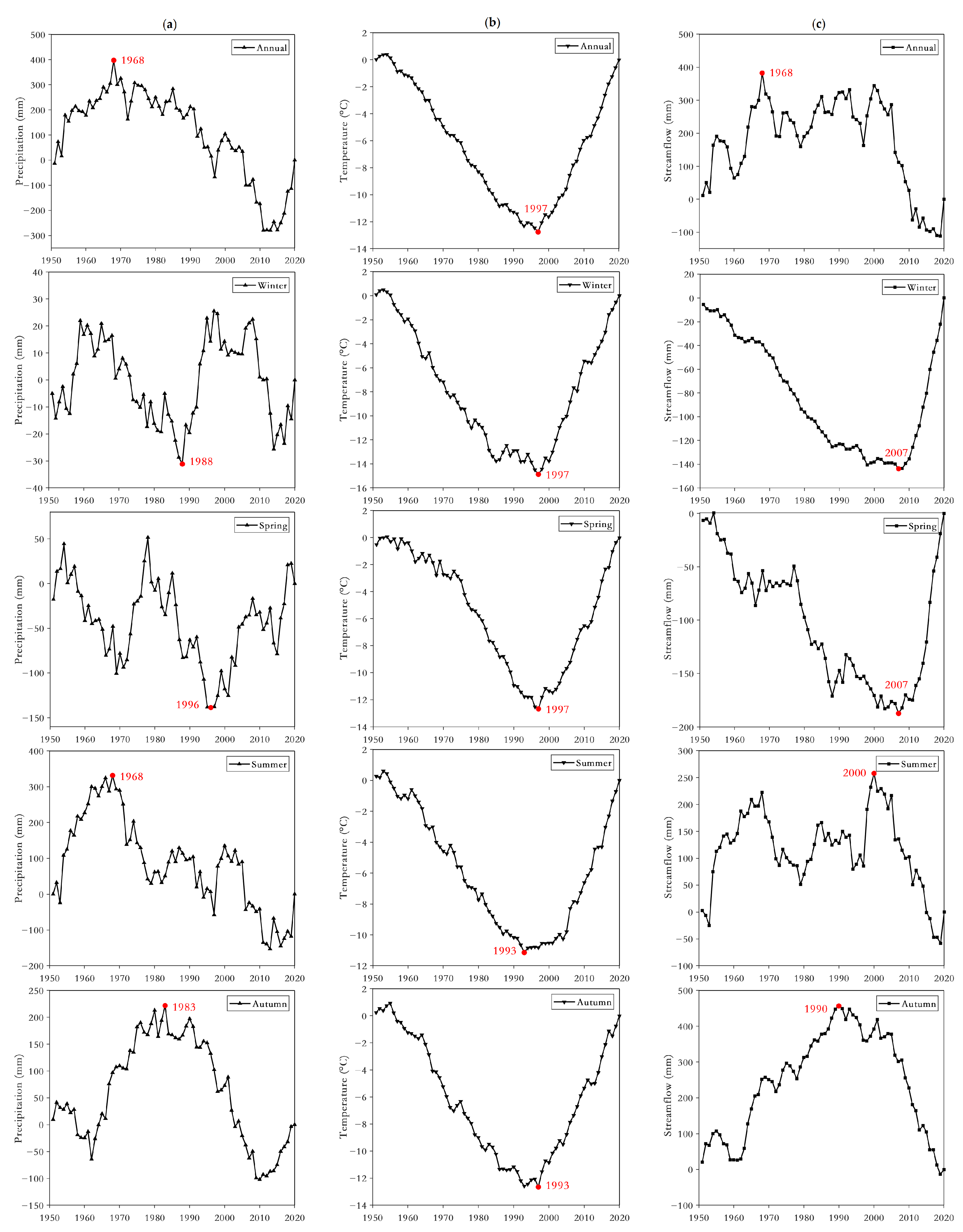
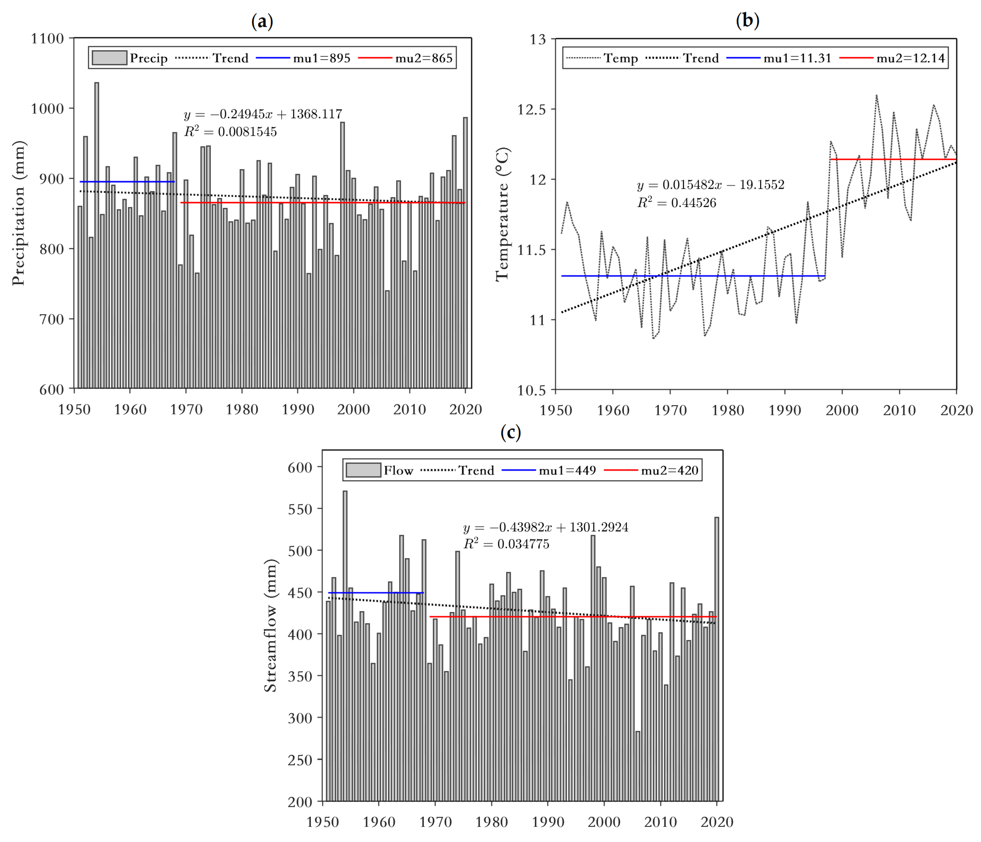
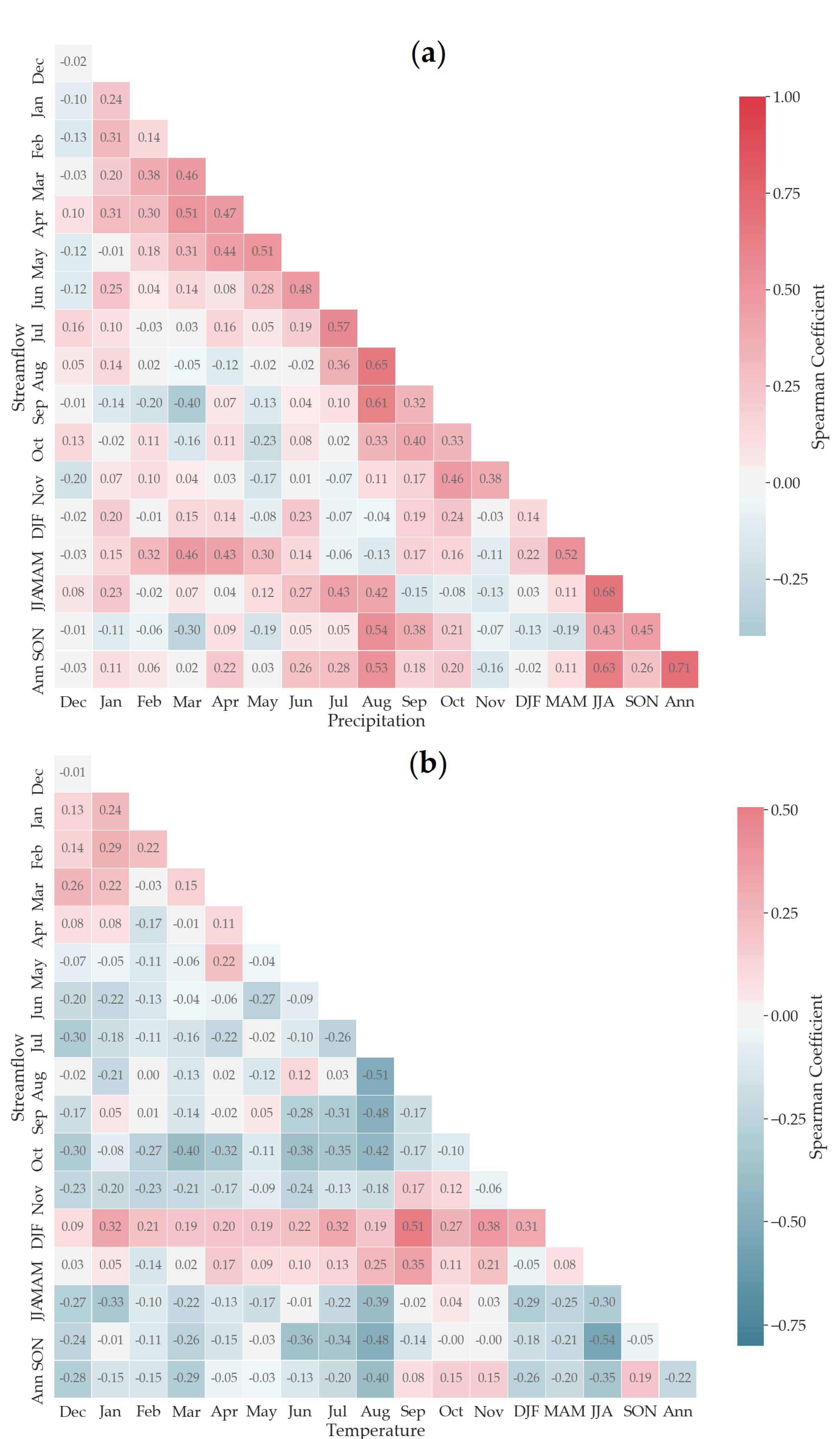
Publisher’s Note: MDPI stays neutral with regard to jurisdictional claims in published maps and institutional affiliations. |
© 2022 by the authors. Licensee MDPI, Basel, Switzerland. This article is an open access article distributed under the terms and conditions of the Creative Commons Attribution (CC BY) license (https://creativecommons.org/licenses/by/4.0/).