Abstract
Particulate matter (PM) emitted from livestock and poultry production contributes to atmospheric aerosol loading, affecting animal health and the surrounding atmospheric environment. However, developing and optimizing remediation technologies require a better understanding of air pollutant concentrations, the emission plumes, and the mechanism of emission. Previous studies have primarily focused on indoor air pollution research, while outdoor research is relatively rare. Field test research is not only costly but also consumes extensive amounts of time. The application of computational fluid dynamics (CFD) technology can save a lot of measurement time and repetitive labor, in order to better understand the diffusion fundamentals and spatial and temporal distribution differences of PM. This study monitored the PM concentrations of different particle sizes inside and outside a layer house with negative pressure ventilation in Northeast China during the summer of 2021. These data were also used to validate the three-dimensional simulation of the PM concentrations inside and outside of the layer house in various scenarios of wind directions at different times by CFD technology. Through correlation analysis, it is found that temperature was positively correlated with PM1 and PM2.5, and relative humidity and wind speed were negatively correlated with PM, which has a greater impact on PM10 and total suspended particulate (TSP). The particle size was proportional to the diffusion distance and diffusion height, time, and wind direction both have an impact on the spread of PM. Considering the environmental conditions in Northeast China, increasing the height of the fan by 1 m was suggested to reduce the diffusion of PM concentration. In addition, the diffusion patterns and transport paths in this study provide valuable information for improving control measures to minimize the influence of PM on both animal health and air quality.
1. Introduction
The livestock and poultry breeding industry is an important section in the development of the agricultural economy. With the introduction of internet technology and modernized breeding management technologies in the industrial chain, the Chinese livestock and poultry breeding industry has shown a trend of rapid development [1]. In 2020, the number of laying hens in China increased to 6.78 billion, a year-on-year increase of 3.99%. In the past 30 years, China has been the world’s largest egg producer, accounting for nearly 40% of the world’s egg production [2]. Previously, air pollution caused by PM was generally regarded as a consequence of industrialization and urbanization, and agriculture was not regarded as the main source of air pollution. However, the latest European studies [3] have shown that agriculture may be one of the main sources of air pollution; particularly, PM from livestock and poultry farming is one of the main sources of agricultural PM. With the development of livestock and poultry farming, its PM emissions will take a larger weighting accordingly.
PM is generally categorized as total suspended particulate (TSP), PM with an aerodynamic equivalent diameter of less than 10 μm (PM10), PM with an aerodynamic equivalent diameter of less than 2.5 μm (PM2.5), and PM with an aerodynamic equivalent diameter of less than 1μm (PM1). The main source of poultry house emissions is layer house litter, which is a mixture of manure, waste food, feathers, and other litter [4]. The microorganisms in the layer house rely on the relative stability of the colloidal dispersion system and use PM as the medium to spread, which affects the health of the animals and staff in the house. There is about 6.1 × 10⁵ CFU microbial aerosol in the layer house every day carrying bacteria that is able to enter the lungs of humans and animals [5]. PM can also be discharged into the atmosphere through a mechanically ventilated exhaust system, polluting the surrounding atmospheric environment. High concentrations of environmental PM can cause atmospheric environmental problems, such as the formation of acid rain, radiation concentration, and reduced atmosphere visibility. PM discharged outside the layer house also carry various odor molecules, bacteria, viruses, and other biological components. PM can be spread to the surrounding environment with the air, causing serious harm to the health of surrounding residents [6,7]. In summer, when the temperature is high, it is essential to increase the ventilation to remove the excess heat in the house. A higher ventilation rate results in a higher emission rate of PM from inside to the outdoor atmosphere, that is, PM generated in the house is more emitted to the atmospheric environment outside. The particle concentrations of indoor and outdoor were highly correlated in summer, and more than 60% of indoor PM may be transported to the outdoor environment [8]. For layer houses, the air pollution caused by PM in summer is much greater than that in winter [9].
As an aerosol system, PM has all the properties of general aerosol pollutants that follow the diffusion and propagation of the atmosphere, and their movement changes also follow the turbulent diffusion law. The final factor that determines the rate of atmospheric dilution and diffusion is the nature of atmospheric motion, namely, wind and turbulence [10]. Many studies have focused on the influence of wind speed on atmospheric diffusion [11,12,13,14] including the effects of different wind speed conditions on the temporal and spatial distribution of pollutant concentration, particle uplift height, and pollutant diffusion range of single point source emissions. In fact, wind direction also directly affects the strength of turbulent activity, which in turn affects the transportation and diffusion of pollutants. Exploring the diffusion law of PM at different wind speeds and wind directions is crucial to a better understanding of air pollutant concentrations, and the diffusion patterns and transport paths.
A number of studies have been conducted on PM in layer houses, which mainly focus on monitoring the concentration of PM inside layer houses, determining the source of PM in layer houses, and developing measures to reduce dust in layer houses. In the meantime, studies on the diffusion law and propagation path of PM outside layer houses are limited. In particular, little research has been conducted concerning the PM emission plume characteristics and PM concentrations downwind from the mechanical ventilation. Before strategizing control and remediation techniques, it is crucial to characterize these emission plumes and to record critical interactions between the pollutants and environmental conditions which influence their dispersion. Compared with field test research, the application of CFD technology can save a lot of measurement time and repetitive labor, in order to better understand the diffusion fundamentals and spatial and temporal distribution difference of PM. Therefore, we modeled the house by three-dimensional modeling using CFD technology. Numerical simulation analysis on the PM concentration inside and outside was conducted to explore the distribution and propagation path of PM to provide a theoretical basis for improving the environmental quality of livestock and poultry houses.
2. Materials and Methods
2.1. Layer House
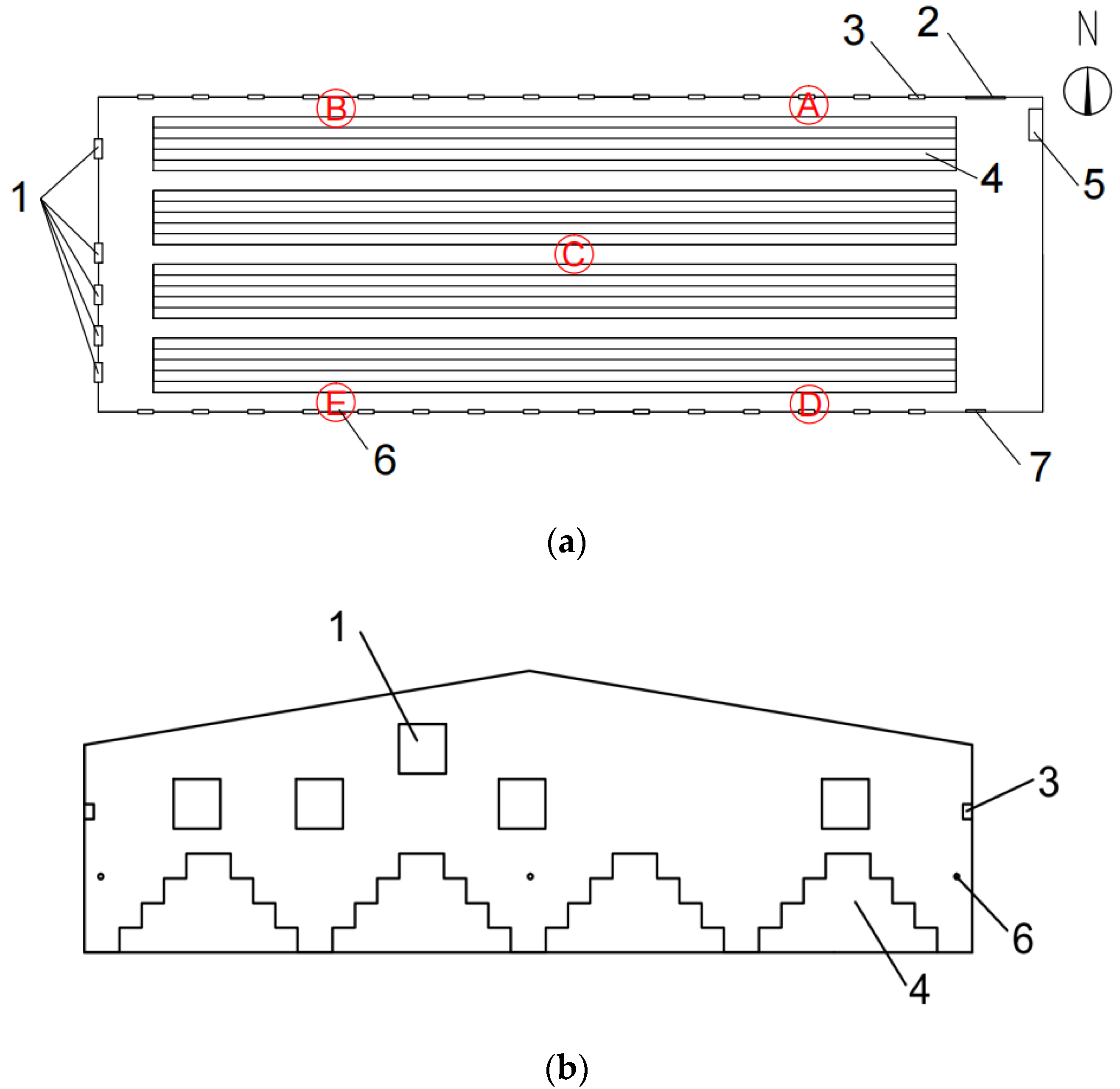
The layer house selected for experimental tests is located at a laying hen breeding base in Jilin Province, China. The layer house is an east–west and steel–concrete building with a length of 55 m, a span of 16 m, eaves height of 4.2 m, and ridge height of 6 m. Negative-pressure longitudinal ventilation was adopted. There are five BNM-1460 fans (height × width × thickness: 1460 × 1460 × 600 mm; blade diameter: 1220 mm) on the west wall and fifteen 0.5 × 0.3 m vents on the north and south walls. The east wall had a 1.2 × 2.1 m door. The south wall and the north wall each had a wet curtain, which measured 1.5 × 3 m and 1.5 × 1.5 m (Figure 1), respectively. The chicken flocks during experimental tests were 44-week-old “Hailan Brown” laying hens with a total of 12,080 chickens, which were reared in four rows with four layers in a stepped manner and five aisles. The feeding time was 7:00, 11:00, and 16:00 daily. The conveyor belt automatically cleans the manure, which is directly transmitted to the outdoors and transported to the manure storage tank by the manure removal truck.
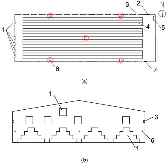
Figure 1.
Layouts of layer house and measurement locations: (a) plane figure of the layer house; (b) section plan of the layer house. (1) fans, (2) wet curtain on the north side, (3) air vent, (4) laminate chicken cage, (5) inner door, (6) measurement point with a vertical height of 1.5 m, they are A, B, C, D and E, and (7) wet curtain on the south side.
2.2. Field Measurement
The experiment was conducted from 12 to 21 July 2021. The daily monitoring time was 06:00–24:00. During the test, all five fans were turned on. A high-precision temperature and humidity recorder (SSN-22, Shenzhen Yuyuan Plus One Sensor System Co., Ltd., Shenzhen, China) was used to continuously collect the measurement point temperature and humidity data. Wind speed data used a Ulide (UNI-T) UT363° mini-type digital anemometer (range: 0–30 m/s; resolution: 0.1 m/s). Dust Truck DRX Desktop (Model 8533, TSI Incorporated, Shoreview, MN, USA) was used to monitor the concentration of PM. The accuracy of PM concentration was ±0.001 mg/m3. This instrument has the characteristics of simultaneously detecting PM1, PM2.5, PM10, and TSP.
The measuring points were distributed in 5 monitoring points inside the layer house (Figure 1a) and 30 monitoring points outside the house in Figure 2. The 5 measuring points in the house are located in the south and north aisles and the middle position of the layer house, with a height of 1.5 m. Outside the house, 30 monitoring points with a vertical height of 1 m and 2 m are set up at a horizontal distance of 0.5 m, 1.5 m, 3 m, 6m, and 11 m from the center of the west wall of the layer house. The temperature, relative humidity, and wind speed in the layer house were monitored every 2 h. Inside and outside PM concentrations were collected every 10 min and 1 h, respectively. Sequential measurement was conducted from point 1 to point 30 outside the house, and each point was monitored for 2 min, and it was cycled every 1 h. The monitoring of the inside and outside points were simultaneous. The thermometer, hydrometer, and anemometer were selected in the same position as the PM monitor to facilitate real-time monitoring of the temperature, relative humidity, and wind speed, respectively.

Figure 2.
Distribution of measurement points outside the layer house. Thirty sampling locations (S1~S30) with 2 different sampling heights (1 m and 2 m) were deployed perpendicularly downwind of the primary fan. S2 and S6 were 1 m from S4 on either side; S8 and S12 were 2 m from S10 on either side; S14 and S18 were 3 m from S16 on either side; S20 and S24 were 4 m from S22 on either side; and S26 and S30 were 5 m from S28 on either side. The points were parallel to the layer house.
2.3. Numerical Simulation
2.3.1. Layer House Model
The closed half-step cage layer hen house was modeled using 3D software with 1:1 scale. In order to improve the operating efficiency of the Fluent software, the 4 breeding lines in the house were simplified into 4 rectangles. All of the chickens in each cage were simplified to a rectangular parallelepiped with the same length as the cage, and feeding and manure removal equipment were omitted. Taking into account the computing performance of the computer, the outside computational domain of the layer house had dimensions of 110 (length) × 80 (width) × 40 m (height). The air was set as an incompressible ideal gas [15].
2.3.2. Grid
An unstructured tetrahedral grid was used, and the grid convergence index (GCI) was used to quantify the uncertainty of grid convergence [16]. After the grid independence test, it was determined that the maximum grid size was 359 mm. For accurate calculation of air inlet and fan, the air inlet and fan area of the layer house were divided separately, and the maximum local grid size was 28 mm. The number of divided grid units was 86,349,117, the number of nodes was 9,473,623, and the number of overall grids was 15,715,546.
2.4. Boundary Conditions
The main sources of PM in the layer house include dander, feed, manure, and waste [17], most of which come from the chicken body itself and the area around the chicken. In this simulation, the position of the simplified rectangular parallelepiped of the chicken and the chicken cage was used as the particle release source area, and the non-slip wall was set. The initial mass concentration of the particle source obtained by measuring was set to PM1: 0.4 mg/m3, PM2.5: 0.6 mg/m3, PM10: 3.7 mg/m3, and TSP: 5.5 mg/m3. The specific settings of other boundary conditions by measuring are listed in Table 1.

Table 1.
Boundary condition setting.
2.5. Fundamental Conservation Equation
Mass conservation equation:
where refers to vector operator, ; refers to fluid density (kg/m3); refers to time (s); refers to speed (m/s); and refers to quality source term [kg/(m3·s)].
Momentum conservation equation:
where refers to pressure (Pa); refers to gravity term (N/m3); and refers to external force, (N/m3).
Energy conservation equation:
where refers to total fluid energy (J); refers to thermal conductivity [W/(m·K)]; refers to temperature (°C); refers to specific enthalpy (J/kg); refers to diffusion flux [kg/(m2·s)]; and refers to total entropy (W/m3).
Component transfer equation:
where refers to the mass fraction of component i, which was the mass fraction of water vapor in this article; and refers to water vapor quality source term [kg/(m3·s)].
2.6. Turbulence Model
Seo et al. [18,19] and Lee et al. [20] found that the renormalized group RNG k-ε turbulence model can effectively express the flow field distribution in the layer house. In this simulation study, the Fluent 19.0 software was used for numerical solution, and the high-precision renormalization group RNG k-ε turbulence model was selected to carry out the numerical simulation. The simulation of the near-wall area adopts the standard wall function, and the control equation adopts the discrete method based on finite volume. The pressure–velocity coupling uses the SIMPLEC algorithm, the momentum and turbulence energy use the second-order upwind discrete format, and the discrete phase model (DPM) was set for PM.
2.7. Force Analysis of Particles in the Flow Field
The force on the particles in the fluid is the fundamental reason to change their motion state. Understanding the source term of the particle force is the theoretical basis for establishing the numerical simulation. The movement of particles in the airflow is affected by the fluid force of the airflow on the particles, the collision and frictional forces between particles and other objects, as well as some external interference field forces. Forces can be roughly divided into inherent forces such as gravity, inertial force, etc., caused by particle movement, relative movement between particles and fluid, and interaction between particles, longitudinal forces such as resistance and Basset force along the direction of relative movement, and lateral forces such as Magnus and Saffman along perpendicular to the direction of relative motion. Since this study focused on the movement of dust during the falling process of particles, the forces considered were mainly gravity and inertia and the lift and resistance of the airflow to the particles [21,22,23].
2.8. Data Analysis
In order to analyze and evaluate the accuracy of the CFD simulation, the normalized mean squared error (NMSE) index [24] was used for verification. When the NMSE value was less than 0.25, the simulation accuracy of the CFD could be reasonably considered [25].
where refers to the relative error between the simulated value and the tested value; refers to simulation value; refers to tested value; refers to the average of simulated values; refers to average of tested values; and refers to the number of measured samples.
Statistical analyses of data included one-way ANOVA, Pearson correlation analysis, linear regression, mean and standard deviation, and were performed using SPSS (22.0, IBM Corporation, Armonk, NY, USA) and Microsoft Excel.
3. Results and Discussions
3.1. Analysis of Measured Data
The temperature in the house varied from 21.7 °C to 25.2 °C, and the average temperature was 23.6 °C. Studies found that the comfortable range of temperature in the layer house was 18–25 °C [26], and the temperature in the experimental house was suitable for layer growth. The relative humidity in the house varied from 59.9% to 67.1%, and the average humidity was 63.57%. The range of wind speed in the house was 1.42~1.71 m/s, and the average wind speed was 1.5 m/s. Studies have shown that the wind speed in the layer house in summer should not exceed 3 m/s, and the wind speed in the house meets the requirements of production and growth. The average temperatures of the daytime experiments were significantly higher than the average temperatures of the nighttime experiments (p < 0.05). Substantial variability in the relative humidity was observed between all the experiments, but in general, the relative humidity was higher during the nighttime experiments (Table 2).

Table 2.
Average ambient meteorological conditions and PM concentrations during each of the ten daytime inside, daytime outside, and nighttime outside experiments.
TSP mass includes the mass of PM10, PM2.5, and PM1, and thus, the emission of TSP, PM10, PM2.5, and PM1 should be correlated. Linear regression analysis was conducted between TSP and PM10 concentrations, TSP and PM2.5 concentrations, TSP and PM1 concentrations, PM10 and PM1 concentrations, and PM2.5 and PM1 concentrations at different sampling points (Table 3). The results showed that TSP and PM10 were strongly correlated (R2 = 0.83, p < 0.001), demonstrating that the TSP concentrations can be a good indicator for PM10 concentrations, which were easier to sample and analyze. However, the correlation between TSP and PM2.5 concentrations was not as strong (R2 = 0.69, p < 0.05). It was possible that PM2.5 with a much smaller mass was dispersed more readily and that the PM2.5 was more susceptible to the influence of the atmospheric environment and the correlation between TSP and PM1 was worse (R2 = 0.53 p < 0.05). However, the PM2.5 and PM1 concentrations were strongly correlated (R2 = 0.91, p < 0.001), demonstrating the same concentrations as small-sized particles, with the same changing law. The concentration of PM in the atmosphere at nighttime was lower than daytime. The main reason was that the laying hens sleep at nighttime, and compared with daytime, the activity of the flock significantly reduced, resulting in a reduction in the PM content in the house; therefore, the concentration of PM emitted into the atmosphere was also reduced.

Table 3.
Pearson correlation coefficients between PM (TSP, PM10, PM2.5, and PM1) concentrations and the corresponding potential influential factors (temperature, relative humidity, and wind speed).
3.2. Comparison of Simulated and Measured Data
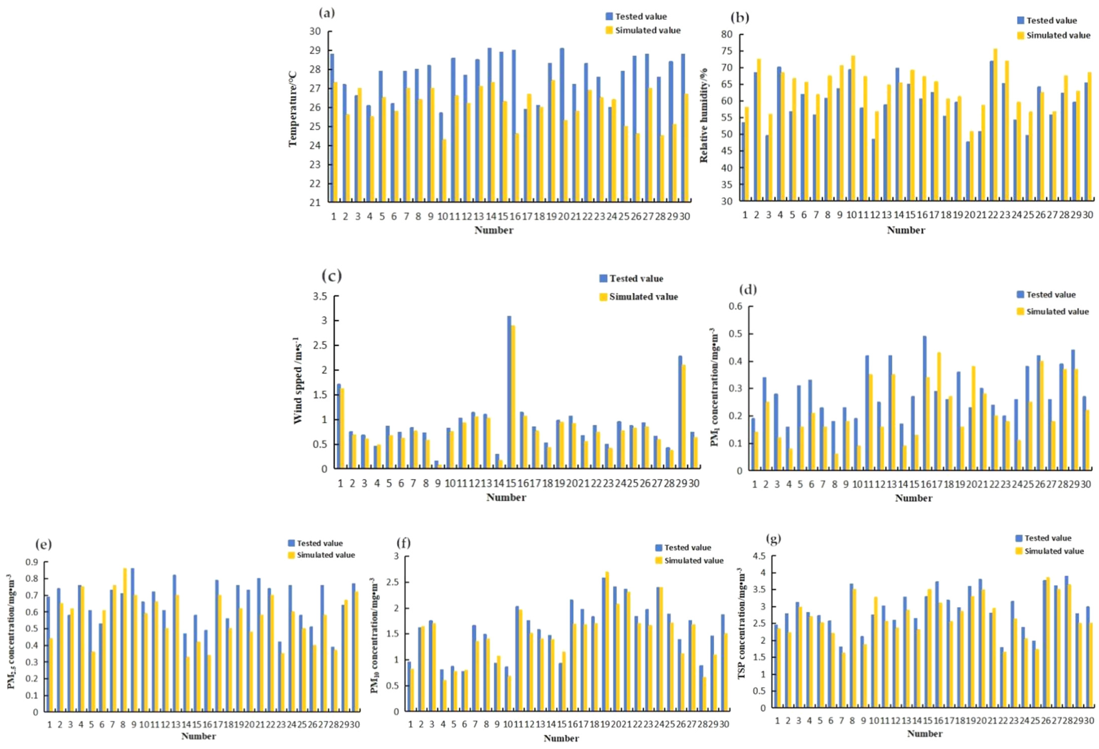
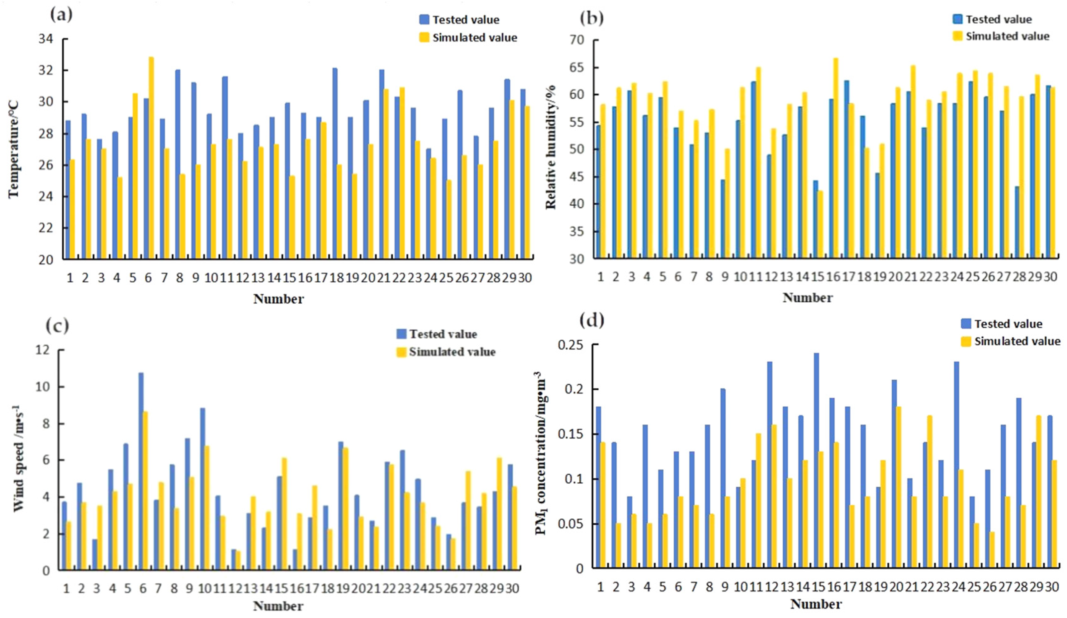
The results of the comparison between the simulated value and the tested value of this simulation are shown in Figure 3 and Figure 4. The comparative analysis found that the relative error range of the simulated and measured temperature and relative humidity in the layer house was 1.02~6.23% and 6.19~13.83%. From the comparison results, it can be found that the temperature simulation value was generally larger than the actual tested value (Figure 3a and Figure 4a), while the simulated relative humidity value was relatively small compared with the actual tested value (Figure 3b and Figure 4b). Because the manure removal port connected to the outdoors was not considered in the simulation process, the simulated temperature values were generally large relative to the measured values. At the same time, the simulation result of the simulated relative humidity was too small because the evaporation of water from feces was not considered. It resulted in the simulated relative humidity value being higher than the actual tested value. The temperature outside the house is more affected by environmental factors than inside. Variation in natural wind speed and direction, as well as changes in cloud and fog, have an impact on the temperature outside the house [27,28]. Environmental factors were not considered in the simulation process, resulting in errors between the simulated and measured values. The overall wind speed in the layer house was small (Figure 3c and Figure 4c), and in the simulation process, we only consider the main ventilation position, but other positions in the layer house also have air exchange, so the wind speed simulation result was too small. The relative error of the calculation result was within a reasonable range, and the simulation result was more reliable, which can accurately reveal the distribution of temperature, relative humidity, and wind speed field forces in the layer house.
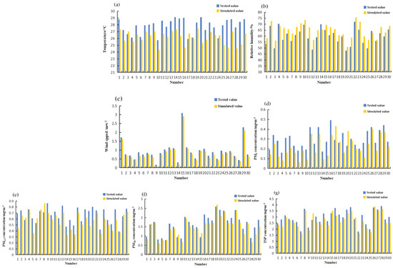
Figure 3.
Measured value compared with simulated value: (a) temperature; (b) relative humidity; (c) wind speed; (d) PM1; (e) PM2.5; (f) PM10; and (g) TSP (inside).
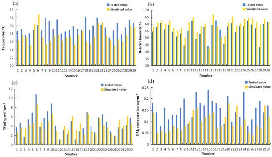

Figure 4.
Measured value compared with simulated value: (a) temperature; (b) relative humidity; (c) wind speed; (d) PM1; (e) PM2.5; (f) PM10; and (g) TSP (outside).
The relative error ranges of the simulated and tested values of PM1, PM2.5, PM10, and TSP in the layer house are 4.26~32.47%, 7.16~29.64%, 5.67~30.32%, and 6.86~43.29%, respectively. The error of TSP was the biggest, this was because the simulation process only considers the PM produced by the feed, ignoring the PM produced by feces, feathers, etc., which leads to errors. Compared with the inside of the house, the atmospheric environment outside was more complicated. The PM outside the house comes from the inside of the layer house [29], so the reason for the error was the same as that of the inside. The relative error and the NMSE value are both larger than that of the inside, but comparing the simulation with the measured data, the NMSE values are all less than 0.25, so there was no significant difference between the simulated value and the tested value, and the simulation results are within an acceptable range, indicating that the CFD layer house particle simulation model was reasonable and usable. Other relative error values and NMSE values are shown in Table 4 and Table 5.

Table 4.
The relative error and normalized mean squared error (NMSE) value of temperature, relative humidity, wind speed, and PM concentration (inside).

Table 5.
The relative error and normalized mean squared error (NMSE) value of temperature, relative humidity, wind speed, and PM concentration (outside).
3.3. Evaluation of Simulation Results
3.3.1. PM Concentration Measurements and Profiles Indoor
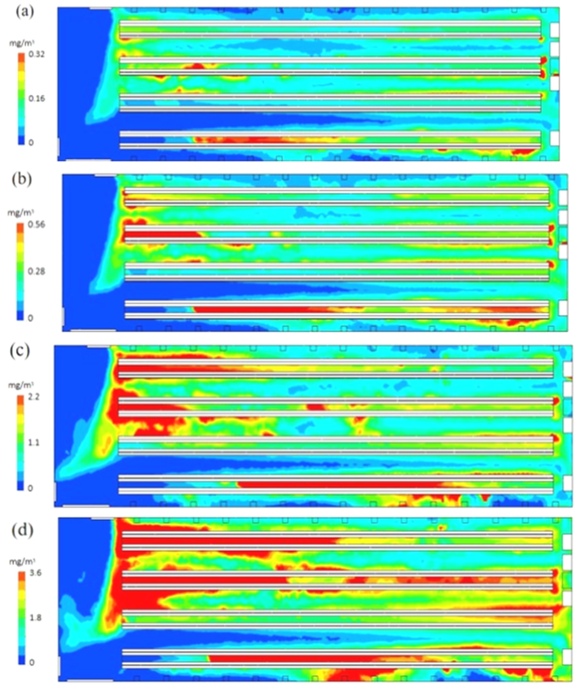
The PM1, PM2.5, PM10, and TSP concentration distribution diagram in the cross section of the layer house with a vertical height of Z = 1.5 m is shown in Figure 5. From the simulation results, the range of PM1 concentration was 0~0.32 mg/m3, PM2.5 concentration was 0~0.4 mg/m3, PM10 concentration was 0~2.2 mg/m3, and TSP concentration was 0~3.6 mg/m3. The PM concentration value obtained by the simulation was basically consistent with the data value measured by the experiment. For the PM of various sizes, the temperature was reduced in the summer by increasing the wind speed, so that the overall distribution of the PM was more uniform. The concentration on the north side was slightly higher than that on the south side. This was due to the higher wind speed at the door, which forms strong convection with the fan on the north side. The wind speed drives more PM to flow from the north side, and was finally discharged to the atmosphere through the north side fan. This process makes the PM easy to form and accumulate under the barrier of the chicken shelves. The concentrations of PM10 and TSP were higher at the location far away from the fan. This was because the longer the layer house, the more likely the PM would form a continuous closed loop along the x direction, and the PM would accumulate on the other side of the fan [30].
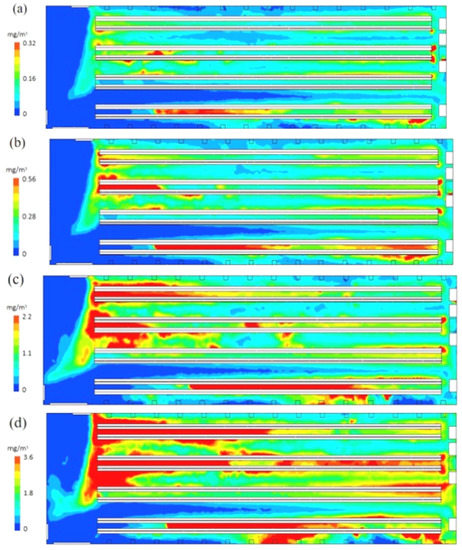
Figure 5.
PM concentration distribution contours at Z = 1.5 m heights by CFD technology: (a) PM1; (b) PM2.5; (c) PM10; and (d) TSP (inside).
3.3.2. PM Concentration Measurements and Profiles Outdoor
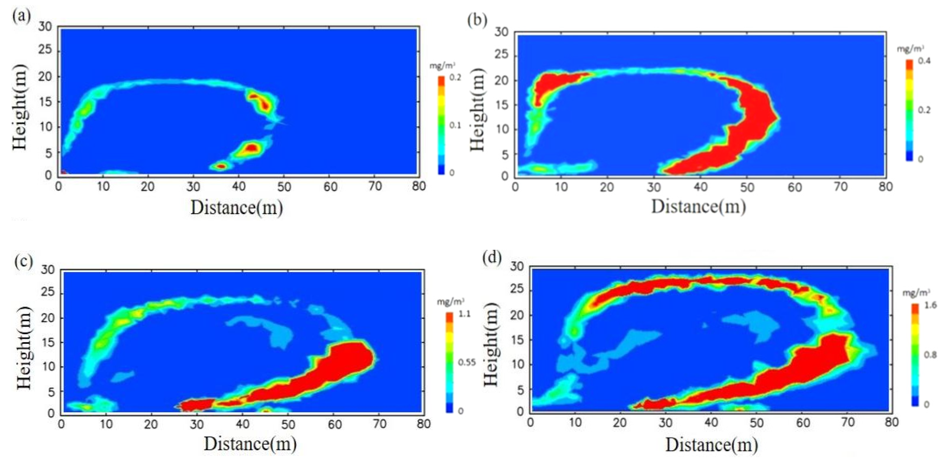
The figures show the cross section of the PM1, PM2.5, PM10, and TSP particle concentration distribution diagram taken from the outside of the layer house, vertically, and the middle position of the fan surface (Y = 0) (Figure 6), and the vertical height of Z = 1.5 m outside (Figure 7). The average PM concentrations for the simulation values were from 0 to 0.2 mg/m3 for PM1, 0 to 0.4 mg/m3 for PM2.5, 0 to 1.1 mg/m3 for PM10, and 0 to 1.6 mg/m3 for TSP. The direction of the measured PM emission plumes was dominated by the airflow rate and the orientation from the mechanical ventilation. As shown in the simulation diagram, the larger the particle size, the longer the diffusion distance in the atmosphere, and the higher the transmission height. The speed generated by the rotation of the impeller of the fan uses the relationship between the pressure rise and the speed to generate a pressure difference between the inside and the outside of the house [31]. The physical properties of the density of particles that are lower than the atmospheric density of the external environment lead to diffusion in the atmospheric environment under specific conditions with initial momentum, pressure difference, and temperature difference. Due to the existence of the pressure difference, the PM was discharged at the position of the fan, which has a speed much higher than the wind speed. In addition, with the effect of buoyancy, the height continues to rise, and the entrainment of the external particles through the entrainment effect causes the momentum to gradually decrease, and the forward speed also decreases, accordingly, until the particle speed drops to the point where there is no longer a speed difference with the outside wind speed; it is mainly affected by buoyancy and atmospheric turbulence. The density of suspendable particles was less than that of air. Therefore, in the external environment, the buoyant force of natural particles by air was greater than the force of gravity, that is, the resultant force in the vertical direction. Therefore, the particles will continue to move upwards. After the particles complete the jetting process under the initial pressure difference, the buoyancy begins to affect the movement of the particles, which further expands the diffusion range of the particles. As time accumulates, the PM under the action of atmospheric turbulence will be entrained and mixed with the outside air, and the volume of the PM will further increase. As the distance along the downwind direction increases, the density of particles increases, and the buoyancy continues to decrease [32].
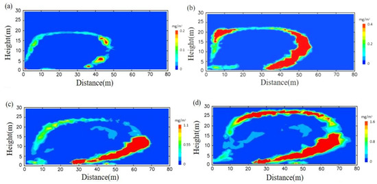
Figure 6.
PM concentration profiles at vertical direction at 30 m heights by CFD technology: (a) PM1; (b) PM2.5; (c) PM10; and (d) TSP (outside).
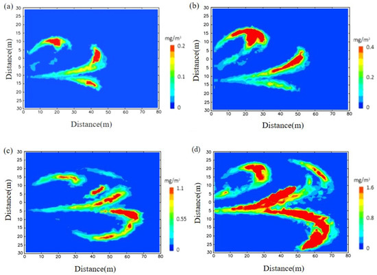
Figure 7.
PM concentration profiles at horizontal direction at 1.5 m heights by CFD technology: (a) PM1; (b) PM2.5; (c) PM10; and (d) TSP (outside).
In addition, the strong solar radiation intensity in summer, ground temperature increase, extremely unstable atmosphere, enhanced turbulent convection in the vertical direction, and strong air diffusion are related [33]. The complexity of the vertical distribution of atmospheric particles was closely related to the atmospheric dynamics, thermal structure, and turbulence characteristics of the boundary layer, as well as local meteorological conditions. In the horizontal distance, due to the influence of gravity and resistance, the particles start to make a projectile motion after rising a certain distance. Because the particles have inertia, and the inertia size is: TSP > PM10 > PM2.5 > PM1, the greater the inertia, the stronger the nature of the particles to keep the motion state unchanged, and the more difficult it is for the motion state to change, so in the vertical height and horizontal distance, the larger the particle size, the longer the diffusion distance. Particle size and density are two important factors that determine the settling velocity within a plume [34]. Due to resistance, the diffusion speed of the PM was gradually decreasing. After spreading for a certain distance in the atmosphere, the velocity will be zero. The common wind direction in northern China in summer was southwest. Under the influence of southwest wind, the PM moves along the southwest direction. That is, the PM moves in the direction and finally sinks to the ground.
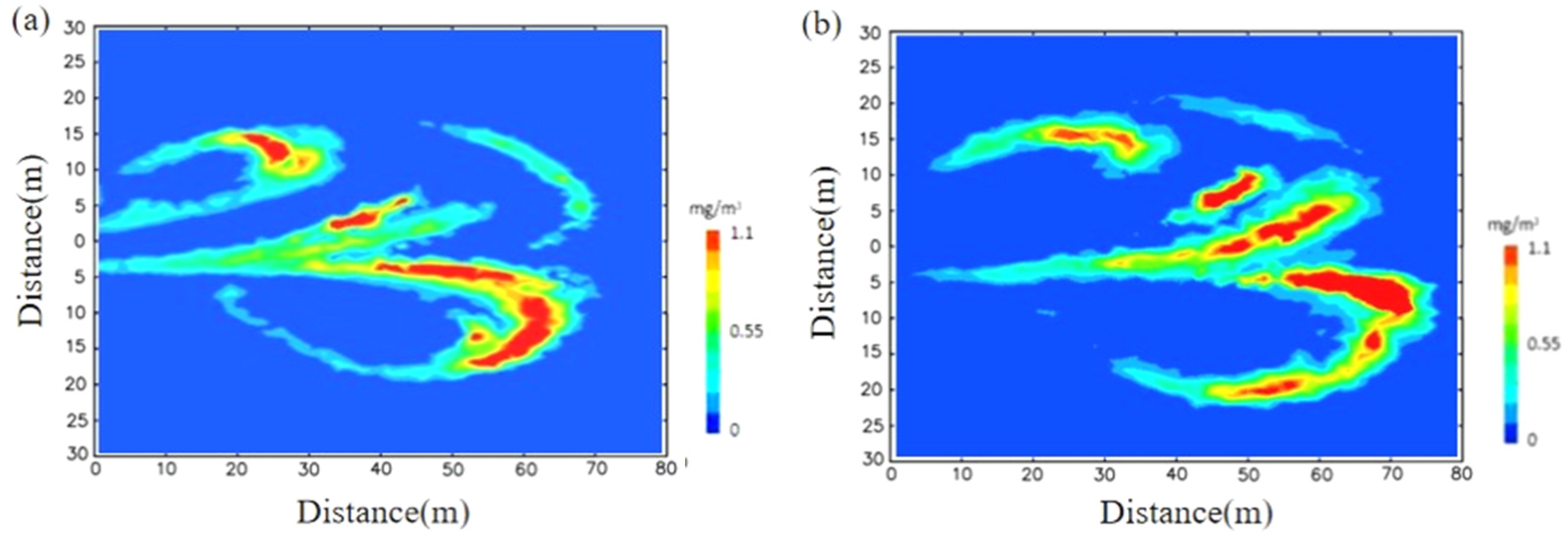
To research the plumes for PM emission patterns in daytime and nighttime, take PM10 as an example (Figure 8). This plume shape was most likely due to the unstable atmospheric conditions during the daytime. During the unstable conditions of the daytime, turbulent diffusion was dominant for PM10 [35]. The atmosphere in the nighttime experiments was much more stable, and this was reflected in the plume shape. Furthermore, molecular diffusion could contribute to the total diffusion of the PM. The horizontal plume shape of PM10 in the nighttime experiments was longer.
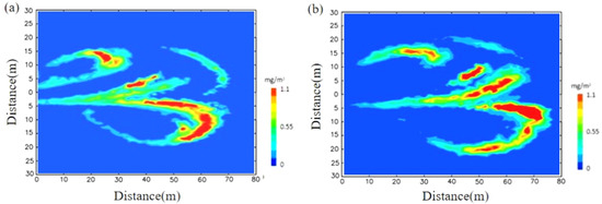
Figure 8.
PM10 concentration profiles at the horizontal direction at 1.5 m heights during daytime and nighttime by CFD technology: (a) daytime and (b) nighttime (outside).
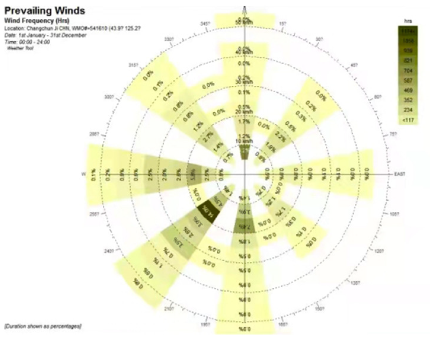
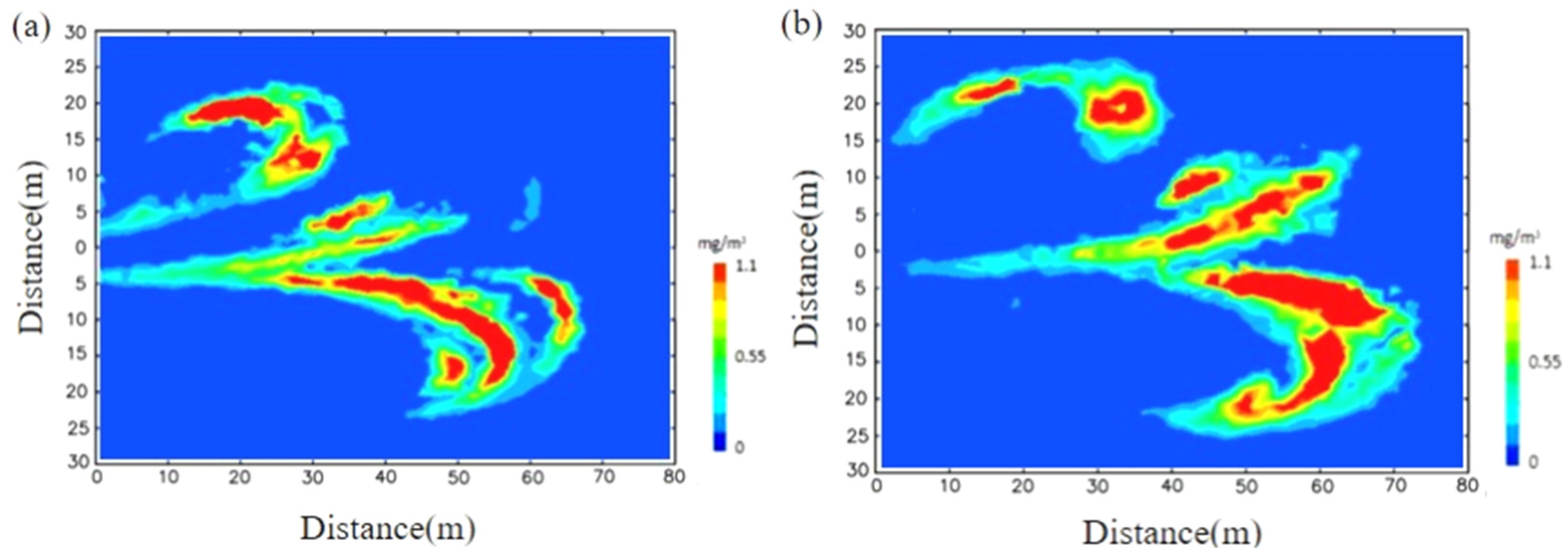
Except for the southwest wind in the main wind direction in summer, according to the wind rose diagram of the test area in Northeast China, the frequency of the southeast wind and northwest wind was second only to the southwest wind (Figure 9). We simulated the influence of southeast and northwest winds on the dispersion of PM when the wind speed was 3 m/s. We intercept the PM diffusion cloud image at a height of 1.5 m from the ground (Figure 10). It can be found that compared with the diffusion distance of the PM under the northwest wind, the distance of the southeast wind spreading downward was longer. This was because the southeast wind direction was the same as the fan exhaust direction, which can better drive the PM to diffuse to the west, indicating that different wind directions have a significant impact on the diffusion distance [36].
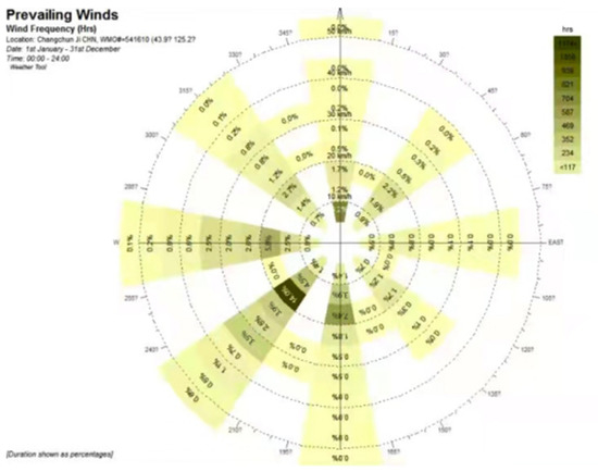
Figure 9.
Wind rose diagram in Northeast China.
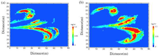
Figure 10.
PM10 concentration profiles at the horizontal direction at 1.5 m height with different wind directions by CFD technology: (a) northwest wind and (b) southeast wind (outside).
3.3.3. Simulated Diffusion Diagram of PM to Increase the Height of the Fan
Through the force analysis and turbulence phenomenon of PM, it can be known that the factor of release height strength was directly related to the distribution of PM concentration [37]. Leakage height has a great influence on the distribution of pollution because as the height increases, PM needs to spread longer to reach the ground, and the ground concentration is significantly reduced after dilution in the process. Leakage height was a parameter that must be considered in the simulation process. We increased the height of the layer house and the upper fan by 1 m, and performed simulation analysis through CFD.
Compared with that before optimization, after optimization, the vertical height and horizontal distance of different particle diameters diffused in the atmosphere have increased (Figure 11). The vertical height of each particle diameter was larger than the range of the calculation domain height of 40 m, indicating the range of diffusion in the vertical height. It exceeded 40 m, and the horizontal diffusion distance still follows: TSP > PM10 > PM2.5 > PM1, and the diffusion distance of TSP and PM10 was greater than 110 m of the computational domain. Due to the limited size of the computational domain, the final diffusion of TSP and PM10 cannot be obtained. Therefore, the relatively short distance of 40 m and 110 m in this study may be insufficient to observe the change in particle size distance. It can be seen from the figure that the high concentration areas of PM are mainly concentrated on high altitudes and near the layer house, and the concentration far away from the fan was significantly lower than before, indicating that as the height of the release source increases, the PM needs to spread longer to reach the ground. In the process of diffusion and settling, the larger the particle size range, the more complicated the diffusion pattern [38]. The ground concentration was significantly reduced when diluted during the process [39,40]. It shows that appropriately increasing the height of the release source helps reduce the concentration of PM when it diffuses to the ground, effectively improving the environmental quality around the livestock and poultry houses, and reducing the harm of PM to the health of residents.
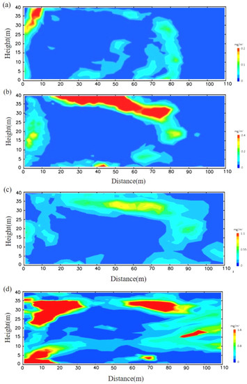
Figure 11.
PM concentration profiles at vertical direction at 40 m height by CFD technology: (a) PM1; (b) PM2.5; (c) PM10; and (d) TSP (outside).
4. Conclusions
Field samples of PM1, PM2.5, PM10, and TSP were monitored during 10-day and 10-night experiments at a commercial poultry production facility in Northeast China. This study analyzed the diffusion law of particles inside and outside a laying hen house under the influence of different conditions by CFD technology. The following conclusions were drawn.
- (1)
- Through correlation analysis, it was found that temperature was positively correlated with PM1 and PM2.5, and relative humidity and wind speed are negatively correlated with PM, which has a greater impact on PM10 and TSP. The correlation between PM10 and TSP was strong, and the correlation between PM1 and PM2.5 was strong. The concentration of PM in the atmosphere at nighttime was lower than daytime.
- (2)
- NMSE and relative error were used to calculate the accuracy of the model, and the relative error and NMSE values are within an acceptable range. The relative error value and the NMSE value outside the house are both larger than those in the house because the atmospheric environment outside the house was more complicated than that in the house, and the turbulence phenomenon was more obvious, which leads to an increase in the simulation error. The PM concentration value obtained by the simulation was basically consistent with the data value measured by the experiment. The concentration on the north side was slightly higher than that on the south side.
- (3)
- The larger the particle size, the longer the diffusion distance in the atmosphere, and the transmission height was dominated by the atmospheric turbulence and the direction of the measured PM emission plumes was dominated by the airflow rate and the orientation from the mechanical ventilation. The horizontal plume shape of PM10 in the nighttime was longer than daytime and when the wind direction was the same as the diffusion direction of the PM, the PM spread farther than other wind directions. Appropriately increasing the height of the release source helps to reduce the concentration of PM when it diffuses to the ground, because the PM is diluted as it descends, effectively improving the environmental quality around the livestock and poultry houses, and reducing the harm of PM to the health of residents.
Author Contributions
Methodology, S.Z.; software, S.Z.; validation, S.Z.; formal analysis, S.Z. and L.Z.; investigation, S.Z., L.J., J.L., B.L., L.Z. and Y.Y.; resources, Y.Y.; data curation, S.Z. and L.Z.; writing—original draft preparation, S.Z.; writing—review and editing, S.Z. and Y.Y.; visualization, Y.Y.; supervision, Y.Y.; project administration, Y.Y.; funding acquisition, Y.Y. All authors have read and agreed to the published version of the manuscript.
Funding
This research was funded by Key-Area Research and Development Program of Guangdong Province (2019B020215002-5).
Institutional Review Board Statement
Not applicable.
Informed Consent Statement
Not applicable.
Data Availability Statement
Publicly available datasets were analyzed in this study.
Acknowledgments
This study was supported by the Research and Development Projects in Key Areas of Guangdong Province of China (2019B020215002-5).
Conflicts of Interest
The authors declare no conflict of interest.
References
- Lin, Y.M.; Wang, H. Development and Application of Information Technology in Dairy Farming. Agric. Technol. 2017, 37, 143. [Google Scholar]
- National Bureau of Statistics of People’s Republic of China. China Statistical Yearbook; National Bureau of Statistics of People’s Republic of China: Beijing, China, 2020. [Google Scholar]
- Nielsen, O.K.; Plejdrup, M.; Winther, M.; Mikkelsen, M.H.; Albrektsen, R.; Nielsen, M.; Fauser, P.; Hoffmann, L.; Hjelgaard, K.; Gyldenkærne, S. Projection of SO2, NOx, NH3 and Particle Emissions-2010–2030; Technical Report from DCE–Danish Centre for Environment and Energy: Aarhus, Denmark, 2012. [Google Scholar]
- Carey, J.B.; Lacey, R.E.; Mukhtar, S. A review of literature concerning odors, ammonia, and dust from broiler production facilities: 2. Flock and house management factors. Appl. Poult. Res. 2004, 13, 509–513. [Google Scholar] [CrossRef]
- Zhong, Z.B.; Wang, N. The Size Distrition and Health Risk Assessment of Microbe Bacterial Aerosol in Livestock and Poultry House. China Anim. Quar. 2014, 31, 101–105. [Google Scholar]
- Bakutis, B.; Monstviliene, E.; Januskeviciene, G. Analyses of airborne contamination with bacteria, endotoxins and dust in livestock barns and poultry houses. Acta Vet. Brun. 2004, 73, 283–289. [Google Scholar] [CrossRef][Green Version]
- Cai, L.; Koziel, J.A.; Lo, Y.C. Characterization of volatile organic compounds and odorants associated with swine barn particulate matter using solid-phase microextraction and gas chromatography-mass spectrometry-olfactometry. J. Chromatogr. A 2006, 1102, 60–72. [Google Scholar] [CrossRef]
- Guo, L.; Zhao, D.S.; Zhao, B.; Ma, S.L.; Liu, X.L.; Li, M.; Liu, X. Seasonal variations and spatial distribution of particulate matter emissions from a ventilated laying hen house in Northeast China. Int. J. Agric. Biol. Eng. 2020, 13, 57–63. [Google Scholar] [CrossRef]
- Redwine, J.S.; Lacey, R.E.; Mukhtar, S.; Carey, J. Concentration and emissions of ammonia and particulate matter in tunnel–ventilated broiler houses under summer conditions in Texas. Trans. ASAE 2002, 45, 1101–1109. [Google Scholar] [CrossRef]
- Huang, Q.; Chen, C.H.; Huang, J.G. Comparison of some stability classifications and the corresponding diffusion parameters. J. Lanzhou Univ. (Nat. Sci.) 1996, 32, 147–154. [Google Scholar]
- Yu, X.M.; Cao, L.; Yan, J.D. A simulation of atmospheric pollution based on multi-phase particle-in-cell method. Sci. Technol. Eng. 2020, 20, 5856–5863. [Google Scholar]
- Jiang, W.M.; Sun, J.N.; Cao, W.J. Course of Air Pollution Meteorology; China Meteological Press: Beijing, China, 2004. [Google Scholar]
- Guo, D.P.; Zhao, P.; Wang, R.; Yao, R.T.; Hu, J.M. Numerical simulations of the flow field and pollutant dispersion in an idealized urban area under different atmospheric stability conditions. Process Saf. Environ. Prot. 2020, 136, 310–323. [Google Scholar] [CrossRef]
- Wang, Y.W.; Zhai, X.F.; Qi, D.L.; Huang, L.; Chen, L. Simulation of the land-use change effect on urban local thermodynamic circulation. Sci. Technol. Eng. 2017, 17, 16–28. [Google Scholar]
- Jiang, X.M.; Zhang, Y.L.; Zhang, X.G.; Huang, L.; Li, F.H.; Wang, J.; Li, H.; Li, M. CFD-based studies on transitional ventilation of closed hen house with semi ladder coop. J. Huazhong Agric. Univ. 2017, 36, 113–120. [Google Scholar]
- Roache, P.J. Quantification of uncertainty in computational fluid dynamics. Annu. Rev. Fluid Mech. 1997, 29, 123–160. [Google Scholar] [CrossRef]
- Dai, P.Y.; Shen, D.; Tang, Q. Research progress on characteristics of particulate matter in livestock houses and its harmful effects on respiratory tract health of livestock and poultry. Sci. Agric. Sin. 2018, 51, 3214–3225. [Google Scholar]
- Seo, I.H.; Lee, I.B.; Moon, O.K. Modelling of internal environmental conditions in a full-scale commercial pig house containing animals. Biosyst. Eng. 2012, 111, 91–106. [Google Scholar] [CrossRef]
- Seo, I.H.; Lee, I.B.; Moon, O.K. Improvement of the ventilation system of a naturally ventilated broiler house in the cold season using computational simulations. Biosyst. Eng. 2009, 104, 106–117. [Google Scholar] [CrossRef]
- Lee, I.; Sase, S.; Sung, S. Evaluation of CFD accuracy for the ventilation study of a naturally ventilated broiler house. JARQ 2007, 41, 53–64. [Google Scholar] [CrossRef]
- Zhi, S. A new centrifugal correction drag force model for gas solid-particle two-phase flow. Powder Technol. 2016, 303, 124–129. [Google Scholar]
- Chung, J.N.; Troutt, T.R. Simulation of particle dispersion in an axisymmetric jet. J. Fluid Mech. 1988, 186, 199–222. [Google Scholar] [CrossRef]
- Sbrizzai, F.; Verzicco, R.; Pidria, M.F.; Soldati, A. Mechanisms for selective radial dispersion of microparticles in the transition region of a confined turbulent round jet. Int. J. Multiph. Flow 2004, 30, 1389–1417. [Google Scholar] [CrossRef]
- Peter, H. Understanding normalized mean squared error in power amplifier linearization. IEEE Microw. Wirel. Compon. Lett. 2018, 28, 1047–1049. [Google Scholar]
- Saraz, J.A.O.; Velasque, H.J.C.; Bedoya, A.E. Thermal evaluation and validati-on of a computational model to unrefined sugar (panela) burner GP150. DYNA 2010, 77, 237–247. [Google Scholar]
- Du, X.Y.; Teng, G.H.; Du, X.D.; Liu, M.L.; Wang, C.Y. Comprehensive evaluation of environmental comfort in layer poultry house using radar graph. Trans. Chin. Soc. Agric. Eng. Trans. CSAE 2020, 36, 202–209. [Google Scholar]
- Bony, S.; Stevens, B.; Frierson, D.M.W. Clouds, circulation and climate sensitivity. Nat. Geosci. 2015, 8, 261–268. [Google Scholar] [CrossRef]
- Chen, W.; Dong, B. Anthropogenic impacts on recent decadal change in temperature extremes over China: Relative roles of greenhouse gases and anthropogenic aerosols. Clim. Dyn. 2018, 52, 3643–3660. [Google Scholar] [CrossRef]
- Guo, L.; Wang, C.; Ma, S.L.; Chen, D.H.; Tong, J.; Ren, L.L. Characterization and influencing factors analysis of indoor and outdoor particulate matter for caged laying hen house with mechanical ventilation. Trans. Chin. Soc. Agric. Mach. 2018, 49, 276–282. [Google Scholar]
- Ma, J.; Liu, Z.Y. CFD simulation and optimization of environmental parametersin closed hen house. J. Shanxi Agric. Univ. (Nat. Sci. Ed.) 2020, 40, 1–9. [Google Scholar]
- Deng, S.H.; Shi, Z.X.; Li, B.M.; Zhao, S.M.; Ding, T.; Zheng, W.P. CFD simulation of airflow distribution in low profile cross ventilated dairy cattle barn. Trans. Chin. Soc. Agric. Eng. 2014, 30, 139–146. [Google Scholar]
- Flagan, R.C.; Seinfeld, J.H. Fundamentals of Air Pollution Engineering; Courier Corporation: North Chemsford, MA, USA, 2012. [Google Scholar]
- Lin, Z.; Hahm, T.S. Turbulence spreading and transport scaling in global gyrokinetic particle simulations. Phys. Plasmas 2004, 11, 1099–1108. [Google Scholar] [CrossRef]
- Yao, Q.; Yang, Z.J.; Li, H.; Buser, M.D.; Wanjura, J.D.; Downey, P.M.; Zhang, C.; Craige, C.; Torrents, A.; McConnell, L.L.; et al. Assessment of particulate matter and ammonia emission concentrations and respective plume profiles from a commercial poultry house. Environ. Pollut. 2018, 238, 10–16. [Google Scholar] [CrossRef]
- Roumeliotis, T.S.; Van Heyst, B.J. Summary of ammonia and particulate matter emission factors for poultry operations. J. Appl. Poult. Res. 2018, 17, 305–314. [Google Scholar] [CrossRef]
- Kim, J.J.; Baik, J.J. A numerical study of the effects of ambient wind direction on flow and dispersion in urban street canyons using the RNG k-ε turbulence model. Atmos. Environ. 2004, 38, 3039–3048. [Google Scholar] [CrossRef]
- Yook, S.J.; Ahn, K.H. Gaussian diffusion sphere model to predict transfer due to diffusional particle deposition on a flat surface in laminar flow regime. Appl. Phys. Lett. 2009, 94, 215. [Google Scholar] [CrossRef]
- Chen, P.Q. Oblique Gaussian Diffusion-Deposition Model and Effect of Gravitational Settlement on Ground Concentration. Environ. Sci. 1982, 1, 61–67. [Google Scholar]
- Sun, T.; Wang, G.B. Discussion on the design of exhaust venting chimney using Gaussian plume model. Chem. Eng. Des. 2018, 1, 12–15. [Google Scholar]
- Fuller, E.N.; Schettler, P.D.; Giddings, J.C. New method for prediction of binary gas-phase diffusion coefficients. Ind. Eng. Chem. 1966, 58, 18–27. [Google Scholar] [CrossRef]
Publisher’s Note: MDPI stays neutral with regard to jurisdictional claims in published maps and institutional affiliations. |
© 2022 by the authors. Licensee MDPI, Basel, Switzerland. This article is an open access article distributed under the terms and conditions of the Creative Commons Attribution (CC BY) license (https://creativecommons.org/licenses/by/4.0/).

