
Spatiotemporal Influences of LULC Changes on Land Surface Temperature in Rapid Urbanization Area by Using Landsat-TM and TIRS Images

 , , ,
, , ,  , and
, and 
Abstract
:1. Introduction
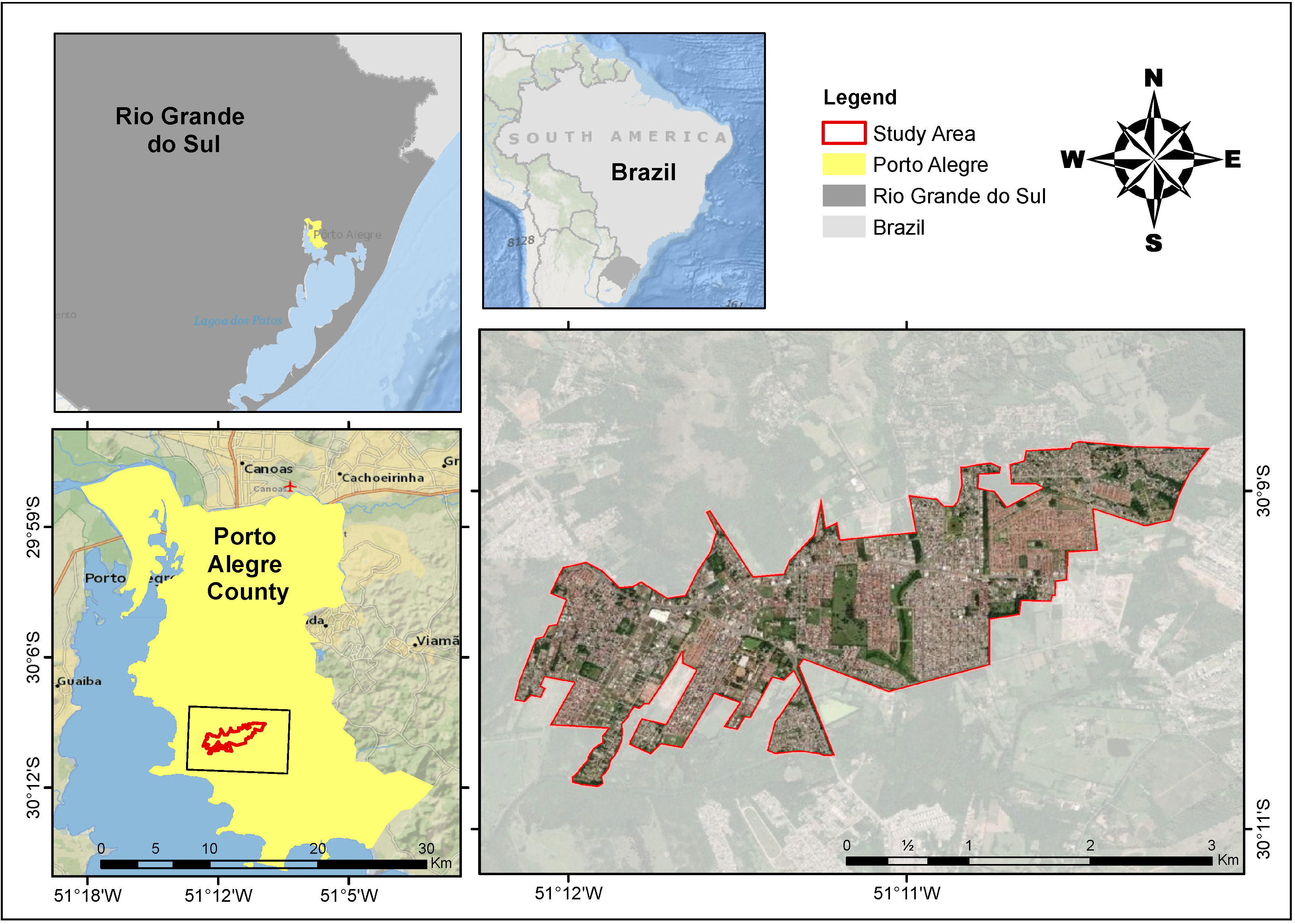
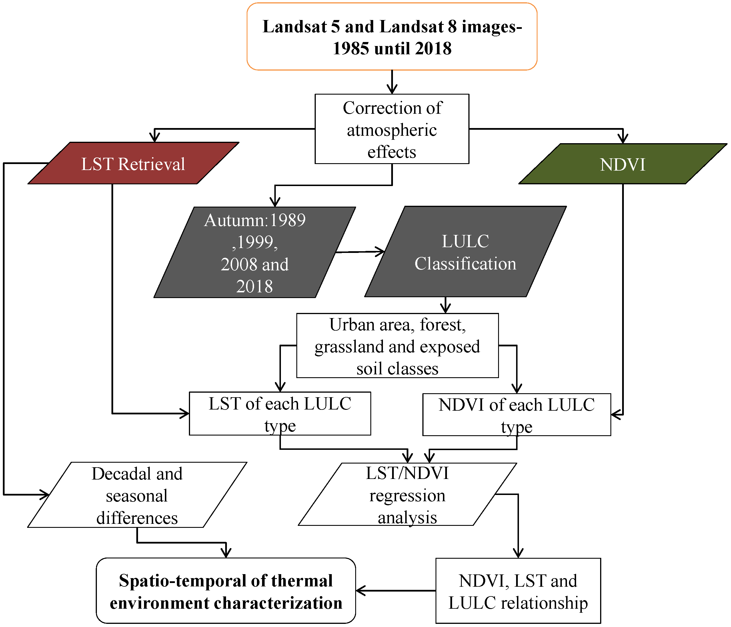
2. Materials and Methods
3. Results
4. Discussion
5. Conclusions
Author Contributions
Funding
Institutional Review Board Statement
Informed Consent Statement
Data Availability Statement
Acknowledgments
Conflicts of Interest
References
- Nations, U. World Urbanization Prospects: The 2014 Revision, Highlights; Department of Economic and Social Affairs, Population Division: New York, NY, USA, 2014; Volume 32. [Google Scholar]
- IBGE, C.D. Censo Demográfico 2010: Características da População e dos Domicílios: Resultados do Universo. 2011. Available online: https://biblioteca.ibge.gov.brvisualizacaoperiodicos93cd_2010_caracteristicas_populacao_domicilios.pdf (accessed on 24 January 2021).
- Tomlinson, C.J.; Chapman, L.; Thornes, J.E.; Baker, C. Remote sensing land surface temperature for meteorology and climatology: A review. Meteorol. Appl. 2011, 18, 296–306. [Google Scholar] [CrossRef] [Green Version]
- Hao, X.; Li, W.; Deng, H. The oasis effect and summer temperature rise in arid regions-case study in Tarim Basin. Sci. Rep. 2016, 6, 1–9. [Google Scholar] [CrossRef] [PubMed]
- Oke, T.R. Boundary Layer Climates; Routledge: London, UK, 2002. [Google Scholar] [CrossRef]
- Andrade, H. O clima urbano-natureza, escalas de análise e aplicabilidade. Finisterra 2005, 40. [Google Scholar] [CrossRef] [Green Version]
- Zhang, Y.; Sun, L. Spatial-temporal impacts of urban land use land cover on land surface temperature: Case studies of two Canadian urban areas. Int. J. Appl. Earth Obs. Geoinf. 2019, 75, 171–181. [Google Scholar] [CrossRef]
- Rasul, A.; Balzter, H.; Smith, C.; Remedios, J.; Adamu, B.; Sobrino, J.A.; Srivanit, M.; Weng, Q. A review on remote sensing of urban heat and cool islands. Land 2017, 6, 38. [Google Scholar] [CrossRef] [Green Version]
- Estoque, R.C.; Murayama, Y.; Myint, S.W. Effects of landscape composition and pattern on land surface temperature: An urban heat island study in the megacities of Southeast Asia. Sci. Total. Environ. 2017, 577, 349–359. [Google Scholar] [CrossRef]
- Bounoua, L.; Zhang, P.; Mostovoy, G.; Thome, K.; Masek, J.; Imhoff, M.; Shepherd, M.; Quattrochi, D.; Santanello, J.; Silva, J.; et al. Impact of urbanization on US surface climate. Environ. Res. Lett. 2015, 10, 084010. [Google Scholar] [CrossRef] [Green Version]
- Norton, B.A.; Coutts, A.M.; Livesley, S.J.; Harris, R.J.; Hunter, A.M.; Williams, N.S. Planning for cooler cities: A framework to prioritise green infrastructure to mitigate high temperatures in urban landscapes. Landsc. Urban Plan. 2015, 134, 127–138. [Google Scholar] [CrossRef]
- Ellison, D.; Morris, C.E.; Locatelli, B.; Sheil, D.; Cohen, J.; Murdiyarso, D.; Gutierrez, V.; Van Noordwijk, M.; Creed, I.F.; Pokorny, J.; et al. Trees, forests and water: Cool insights for a hot world. Glob. Environ. Chang. 2017, 43, 51–61. [Google Scholar] [CrossRef]
- Smith, R.; Choudhury, B.J. On the correlation of indices of vegetation and surface temperature over south-eastern Australia. Int. J. Remote Sens. 1990, 11, 2113–2120. [Google Scholar] [CrossRef]
- Hope, A.S.; McDowell, T. The relationship between surface temperature and a spectral vegetation index of a tallgrass prairie: Effects of burning and other landscape controls. Int. J. Remote Sens. 1992, 13, 2849–2863. [Google Scholar] [CrossRef]
- Julien, Y.; Sobrino, J.A.; Verhoef, W. Changes in land surface temperatures and NDVI values over Europe between 1982 and 1999. Remote Sens. Environ. 2006, 103, 43–55. [Google Scholar] [CrossRef]
- Deng, Y.; Wang, S.; Bai, X.; Tian, Y.; Wu, L.; Xiao, J.; Chen, F.; Qian, Q. Relationship among land surface temperature and LUCC, NDVI in typical karst area. Sci. Rep. 2018, 8, 1–12. [Google Scholar] [CrossRef] [PubMed]
- Kawashima, S. Relation between vegetation, surface temperature, and surface composition in the Tokyo region during winter. Remote Sens. Environ. 1994, 50, 52–60. [Google Scholar] [CrossRef]
- Thanh Hoan, N.; Liou, Y.A.; Nguyen, K.A.; Sharma, R.C.; Tran, D.P.; Liou, C.L.; Cham, D.D. Assessing the effects of land-use types in surface urban heat islands for developing comfortable living in Hanoi City. Remote Sens. 2018, 10, 1965. [Google Scholar] [CrossRef] [Green Version]
- Gallo, K.; McNab, A.; Karl, T.R.; Brown, J.F.; Hood, J.; Tarpley, J. The use of NOAA AVHRR data for assessment of the urban heat island effect. J. Appl. Meteorol. Climatol. 1993, 32, 899–908. [Google Scholar] [CrossRef] [Green Version]
- Yuan, X.; Wang, W.; Cui, J.; Meng, F.; Kurban, A.; De Maeyer, P. Vegetation changes and land surface feedbacks drive shifts in local temperatures over Central Asia. Sci. Rep. 2017, 7, 1–8. [Google Scholar] [CrossRef] [Green Version]
- Rahman, M.; Rony, M.; Hasan, R.; Jannat, F.A.; Chandra Pal, S.; Islam, M.; Alam, E.; Islam, A.R.M. Impact of Urbanization on Urban Heat Island Intensity in Major Districts of Bangladesh Using Remote Sensing and Geo-Spatial Tools. Climate 2022, 10, 3. [Google Scholar] [CrossRef]
- Guha, S.; Govil, H.; Diwan, P. Monitoring LST-NDVI relationship using Premonsoon Landsat datasets. Adv. Meteorol. 2020, 2020, 4539684. [Google Scholar] [CrossRef]
- Abdullah, S.; Barua, D.; Abdullah, S.; Abubakar, M.; Rabby, Y.W. Investigating the Impact of Land Use/Land Cover Change on Present and Future Land Surface Temperature (LST) of Chittagong, Bangladesh. Earth Syst. Environ. 2022, 6, 221–235. [Google Scholar] [CrossRef]
- Fatemi, M.; Narangifard, M. Monitoring LULC changes and its impact on the LST and NDVI in District 1 of Shiraz City. Arab. J. Geosci. 2019, 12, 1–12. [Google Scholar] [CrossRef]
- Gui, X.; Wang, L.; Yao, R.; Yu, D.; Li, C. Investigating the urbanization process and its impact on vegetation change and urban heat island in Wuhan, China. Environ. Sci. Pollut. Res. 2019, 26, 30808–30825. [Google Scholar] [CrossRef] [PubMed]
- Sussman, H.S.; Raghavendra, A.; Zhou, L. Impacts of increased urbanization on surface temperature, vegetation, and aerosols over Bengaluru, India. Remote Sens. Appl. Soc. Environ. 2019, 16, 100261. [Google Scholar] [CrossRef]
- Biswas, S.; Ghosh, S. Estimation of land surface temperature in response to land use/land cover transformation in Kolkata city and its suburban area, India. Int. J. Urban Sci. 2021, 1–28. [Google Scholar] [CrossRef]
- Tayyebi, A.; Shafizadeh-Moghadam, H.; Tayyebi, A.H. Analyzing long-term spatio-temporal patterns of land surface temperature in response to rapid urbanization in the mega-city of Tehran. Land Use Policy 2018, 71, 459–469. [Google Scholar] [CrossRef]
- Marzban, F.; Sodoudi, S.; Preusker, R. The influence of land-cover type on the relationship between NDVI–LST and LST-T air. Int. J. Remote Sens. 2018, 39, 1377–1398. [Google Scholar] [CrossRef]
- Guha, S.; Govil, H. Seasonal variability of LST-NDVI correlation on different land use/land cover using Landsat satellite sensor: A case study of Raipur City, India. Environ. Dev. Sustain. 2021, 1–17. [Google Scholar] [CrossRef]
- Al-Ademomi, A.S.; Okolie, C.J.; Daramola, O.E.; Agboola, R.O.; Salami, T.J. Assessing the relationship of LST, NDVI and EVI with land cover changes in the Lagos Lagoon environment. Quaest. Geogr. 2020, 39, 87–109. [Google Scholar] [CrossRef]
- Frumkin, H. Urban sprawl and public health. Public Health Rep. 2016, 117, 201–217. [Google Scholar] [CrossRef]
- Dubreuil, V.; Quénol, H.; Foissard, X.; Planchon, O. Climatologie Urbaine et Îlot de Chaleur Urbain à Rennes; Ville et biodiversité, Clergeau P. (dir.); Presses Universitaires de Rennes: Rennes, France, 2011; pp. 105–122. [Google Scholar]
- Voogt, J.A.; Oke, T.R. Thermal remote sensing of urban climates. Remote Sens. Environ. 2003, 86, 370–384. [Google Scholar] [CrossRef]
- Weng, Q.; Lu, D.; Schubring, J. Estimation of land surface temperature–vegetation abundance relationship for urban heat island studies. Remote Sens. Environ. 2004, 89, 467–483. [Google Scholar] [CrossRef]
- Chen, X.L.; Zhao, H.M.; Li, P.X.; Yin, Z.Y. Remote sensing image-based analysis of the relationship between urban heat island and land use/cover changes. Remote Sens. Environ. 2006, 104, 133–146. [Google Scholar] [CrossRef]
- Abou El-Magd, I.; Ismail, A.; Zanaty, N. Spatial variability of urban heat islands in Cairo City, Egypt using time series of Landsat Satellite images. Int. J. Adv. Remote Sens. Gis 2016, 5, 1618–1638. [Google Scholar] [CrossRef] [Green Version]
- Keeratikasikorn, C.; Bonafoni, S. Urban heat island analysis over the land use zoning plan of Bangkok by means of Landsat 8 imagery. Remote Sens. 2018, 10, 440. [Google Scholar] [CrossRef]
- Dissanayake, D.; Morimoto, T.; Ranagalage, M.; Murayama, Y. Land-use/land-cover changes and their impact on surface urban heat islands: Case study of Kandy City, Sri Lanka. Climate 2019, 7, 99. [Google Scholar] [CrossRef] [Green Version]
- Lombardo, M. Ilha de Calor nas Metrópoles, o Exemplo de São Paulo. In Ilha de Calor Nas Metrópoles; SA Comércio Indústria: Aveiro, Portugal, 1985. [Google Scholar]
- Coelho, A.L.N.; Correa, W.d.S.C. Temperatura de Superfície Celsius do Sensor TIRS/Landsat-8: Metodologia e aplicações. Revista Geográfica Acadêmica 2013, 7, 31–45. [Google Scholar] [CrossRef]
- Teixeira, D.C.F.; Amorim, M.C.d.C.T. Ilhas de calor: Representações espaciais de cidades de pequeno porte por meio de modelagem. GEOUSP Espaço e Tempo (Online) 2017, 21, 239–256. [Google Scholar] [CrossRef] [Green Version]
- Romero, M.; Baptista, G.; Azevedo, E.; Werneck, D.; Vianna, E.; Sales, G. MudançAs ClimáTicas Ilhas Calor Urbanas; Universidade de Brasília, Faculdade de Arquitetura e Urbanismo: Brasília, Brazil, 2019. [Google Scholar]
- Deosthali, V. Impact of rapid urban growth on heat and moisture islands in Pune City, India. Atmos. Environ. 2000, 34, 2745–2754. [Google Scholar] [CrossRef]
- Xiong, Y.; Peng, F.; Zou, B. Spatiotemporal influences of land use/cover changes on the heat island effect in rapid urbanization area. Front. Earth Sci. 2019, 13, 614–627. [Google Scholar] [CrossRef]
- Suertegaray, D.M.A.; Moura, N.S.V. Morfogênese do relevo do Estado do Rio Grande do Sul. In Rio Grande do Sul: Paisagens e Territórios em Transformação, 2nd ed.; Editora da UFRGS: Porto Alegre, Brazil, 2012; pp. 11–26. Available online: https://lume.ufrgs.br/handle/10183/218532 (accessed on 24 January 2022).
- Ferraro, L.M.W.; Hasenack, H. Carvão e Meio Ambiente; Editora da Universidade/UFRGS: Porto Alegre, Brazil, 2000; Available online: http://multimidia.ufrgs.br/conteudo/labgeo-ecologia/Arquivos/Publicacoes/Livros_ou_capitulos/2000/Centro_de_Ecologia_2000_Carvao_e_Meio_Ambiente.pdf (accessed on 24 January 2022).
- Kuinchtner, A.; Buriol, G.A. Clima do Estado do Rio Grande do Sul segundo a classificação climática de Köppen e Thornthwaite. Disciplinarum Scientia| Naturais e Tecnológicas 2001, 2, 171–182. [Google Scholar]
- Lillesand, T.; Kiefer, R.W.; Chipman, J. Remote Sens. Image Interpret.; John Wiley & Sons: Hoboken, NY, USA, 2015. [Google Scholar] [CrossRef]
- Bailly, J.S.; Arnaud, M.; Puech, C. Boosting: A classification method for remote sensing. Int. J. Remote Sens. 2007, 28, 1687–1710. [Google Scholar] [CrossRef]
- Lu, D.; Weng, Q. A survey of image classification methods and techniques for improving classification performance. Int. J. Remote Sens. 2007, 28, 823–870. [Google Scholar] [CrossRef]
- Qin, Z.; Karnieli, A.; Berliner, P. A mono-window algorithm for retrieving land surface temperature from Landsat TM data and its application to the Israel-Egypt border region. Int. J. Remote Sens. 2001, 22, 3719–3746. [Google Scholar] [CrossRef]
- Jiménez-Muñoz, J.C.; Sobrino, J.A. A generalized single-channel method for retrieving land surface temperature from remote sensing data. J. Geophys. Res. Atmos. 2003, 108. [Google Scholar] [CrossRef] [Green Version]
- Luo, H.; Shao, J.; Zhang, X. Retrieving land surface temperature based on the radioactive transfer equation in the middle reaches of the Three Gorges Reservoir Area. Resour. Sci. 2012, 34, 256–264. [Google Scholar]
- Rozenstein, O.; Qin, Z.; Derimian, Y.; Karnieli, A. Derivation of land surface temperature for Landsat-8 TIRS using a split window algorithm. Sensors 2014, 14, 5768–5780. [Google Scholar] [CrossRef]
- Liu, L.; Zhang, Y. Urban heat island analysis using the Landsat TM data and ASTER data: A case study in Hong Kong. Remote Sens. 2011, 3, 1535–1552. [Google Scholar] [CrossRef] [Green Version]
- Azmi, R.; Saadane, A.; Kacimi, I. Estimation of spatial distribution and temporal variability of land surface temperature over Casablanca and the surroundings of the city using different Landat satellite sensor type (TM, ETMˆ sup+ˆ and OLI). Int. J. Innov. Appl. Stud. 2015, 11, 49. [Google Scholar]
- Isaya Ndossi, M.; Avdan, U. Application of open source coding technologies in the production of land surface temperature (LST) maps from Landsat: A PyQGIS plugin. Remote Sens. 2016, 8, 413. [Google Scholar] [CrossRef] [Green Version]
- Chatterjee, R.; Singh, N.; Thapa, S.; Sharma, D.; Kumar, D. Retrieval of land surface temperature (LST) from landsat TM6 and TIRS data by single channel radiative transfer algorithm using satellite and ground-based inputs. Int. J. Appl. Earth Obs. Geoinf. 2017, 58, 264–277. [Google Scholar] [CrossRef]
- Zanter, K. Landsat 8 (L8) Data Users Handbook; Department of the Interior U.S. Geological Survey: Reston, VA, USA, 2016; p. 33.
- Barsi, J.A.; Schott, J.R.; Hook, S.J.; Raqueno, N.G.; Markham, B.L.; Radocinski, R.G. Landsat-8 thermal infrared sensor (TIRS) vicarious radiometric calibration. Remote Sens. 2014, 6, 11607–11626. [Google Scholar] [CrossRef] [Green Version]
- Cheng, H.-L.; Xia, D.-Q.; Wu, T.-T.; Meng, X.-P.; Ji, H.-J.; Dong, Z.-G. Land Surface Temperature Retrieval from CBERS-02 IRMSS Thermal Infrared Data and Its Applications in Quantitative Analysis of Urban Heat Island Effect. J. Remote Sens. 2006, 33, 702–710. [Google Scholar] [CrossRef]
- Li, Z.L.; Tang, B.H.; Wu, H.; Ren, H.; Yan, G.; Wan, Z.; Trigo, I.F.; Sobrino, J.A. Satellite-derived land surface temperature: Current status and perspectives. Remote Sens. Environ. 2013, 131, 14–37. [Google Scholar] [CrossRef] [Green Version]
- Wang, C.; Myint, S.W.; Wang, Z.; Song, J. Spatio-temporal modeling of the urban heat island in the Phoenix metropolitan area: Land use change implications. Remote Sens. 2016, 8, 185. [Google Scholar] [CrossRef] [Green Version]
- Deilami, K.; Kamruzzaman, M. Modelling the urban heat island effect of smart growth policy scenarios in Brisbane. Land Use Policy 2017, 64, 38–55. [Google Scholar] [CrossRef]
- Li, X.; Zhou, Y.; Asrar, G.R.; Imhoff, M.; Li, X. The surface urban heat island response to urban expansion: A panel analysis for the conterminous United States. Sci. Total. Environ. 2017, 605, 426–435. [Google Scholar] [CrossRef]
- Gilbert, R.O. Statistical Methods for Environmental Pollution Monitoring; John Wiley & Sons: Hoboken, NJ, USA, 1987. [Google Scholar]
- Zhou, W.; Qian, Y.; Li, X.; Li, W.; Han, L. Relationships between land cover and the surface urban heat island: Seasonal variability and effects of spatial and thematic resolution of land cover data on predicting land surface temperatures. Landsc. Ecol. 2014, 29, 153–167. [Google Scholar] [CrossRef]
- Khorchani, M.; Vicente-Serrano, S.M.; Azorin-Molina, C.; Garcia, M.; Martin-Hernandez, N.; Peña-Gallardo, M.; El Kenawy, A.; Domínguez-Castro, F. Trends in LST over the peninsular Spain as derived from the AVHRR imagery data. Glob. Planet. Chang. 2018, 166, 75–93. [Google Scholar] [CrossRef]
- Yue, W.; Xu, J.; Tan, W.; Xu, L. The relationship between land surface temperature and NDVI with remote sensing: Application to Shanghai Landsat 7 ETM+ data. Int. J. Remote Sens. 2007, 28, 3205–3226. [Google Scholar] [CrossRef]
- Hereher, M.E. Effect of land use/cover change on land surface temperatures-The Nile Delta, Egypt. J. Afr. Earth Sci. 2017, 126, 75–83. [Google Scholar] [CrossRef]
- Sabine, C. Ask the Experts: The IPCC Fifth Assessment Report. Carbon Manag. 2014, 5, 17–25. [Google Scholar] [CrossRef]
- Rosenzweig, C.; Solecki, W.D.; Romero-Lankao, P.; Mehrotra, S.; Dhakal, S.; Ibrahim, S.A. Climate Change and Cities: Second Assessment Report of the Urban Climate Change Research Network; Cambridge University Press: Cambridge, UK, 2018. [Google Scholar]
- Revi, A.; Satterthwaite, D.; Aragón-Durand, F.; Corfee-Morlot, J.; Kiunsi, R.B.; Pelling, M.; Roberts, D.; Solecki, W.; Gajjar, S.P.; Sverdlik, A. Towards transformative adaptation in cities: The IPCC’s Fifth Assessment. Environ. Urban. 2014, 26, 11–28. [Google Scholar] [CrossRef]
- Grondona, A.E.B.; Veettil, B.K.; Rolim, S.B.A. Urban Heat Island development during the last two decades in Porto Alegre, Brazil and its monitoring. In Proceedings of the Joint Urban Remote Sensing Event 2013, Sao Paulo, Brazi, 21–23 April 2013; pp. 061–064. [Google Scholar]
- Hashim, B.M.; Al Maliki, A.; Sultan, M.A.; Shahid, S.; Yaseen, Z.M. Effect of land use land cover changes on land surface temperature during 1984–2020: A case study of Baghdad city using landsat image. Nat. Hazards 2022, 1–24. [Google Scholar] [CrossRef]
- Tafesse, B.; Suryabhagavan, K. Systematic modeling of impacts of land-use and land-cover changes on land surface temperature in Adama Zuria District, Ethiopia. Model. Earth Syst. Environ. 2019, 5, 805–817. [Google Scholar] [CrossRef]
- Kafy, A.A.; Al Rakib, A.; Akter, K.S.; Jahir, D.M.A.; Sikdar, M.S.; Ashrafi, T.J.; Mallik, S.; Rahman, M.M.; Faisal, A.A. Assessing and predicting land use/land cover, land surface temperature and urban thermal field variance index using Landsat imagery for Dhaka Metropolitan area. Environ. Chall. 2021, 4, 100192. [Google Scholar]
- Bari, E.; Nipa, N.J.; Roy, B. Association of vegetation indices with atmospheric & biological factors using MODIS time series products. Environ. Chall. 2021, 5, 100376. [Google Scholar]
- Guha, S.; Govil, H. An assessment on the relationship between land surface temperature and normalized difference vegetation index. Environ. Dev. Sustain. 2021, 23, 1944–1963. [Google Scholar] [CrossRef]
- Matsushita, B.; Yang, W.; Chen, J.; Onda, Y.; Qiu, G. Sensitivity of the enhanced vegetation index (EVI) and normalized difference vegetation index (NDVI) to topographic effects: A case study in high-density cypress forest. Sensors 2007, 7, 2636–2651. [Google Scholar] [CrossRef] [Green Version]
- Huete, A.R. A soil-adjusted vegetation index (SAVI). Remote Sens. Environ. 1988, 25, 295–309. [Google Scholar] [CrossRef]
- Gao, X.; Huete, A.R.; Ni, W.; Miura, T. Optical–biophysical relationships of vegetation spectra without background contamination. Remote Sens. Environ. 2000, 74, 609–620. [Google Scholar] [CrossRef]
- Sobrino, J.A.; Julien, Y. Trend analysis of global MODIS-Terra vegetation indices and land surface temperature between 2000 and 2011. IEEE J. Sel. Top. Appl. Earth Obs. Remote Sens. 2013, 6, 2139–2145. [Google Scholar] [CrossRef]
- Rankine, C.; Sánchez-Azofeifa, G.; Guzmán, J.A.; Espirito-Santo, M.; Sharp, I. Comparing MODIS and near-surface vegetation indexes for monitoring tropical dry forest phenology along a successional gradient using optical phenology towers. Environ. Res. Lett. 2017, 12, 105007. [Google Scholar] [CrossRef] [Green Version]
- Khalil, U.; Aslam, B.; Azam, U.; Khalid, H.M.D. Time Series Analysis of Land Surface Temperature and Drivers of Urban Heat Island Effect Based on Remotely Sensed Data to Develop a Prediction Model. Appl. Artif. Intell. 2021, 1–26. [Google Scholar] [CrossRef]
- Sahani, N. Assessment of spatio-temporal changes of land surface temperature (LST) in Kanchenjunga Biosphere Reserve (KBR), India using Landsat satellite image and single channel algorithm. Remote Sens. Appl. Soc. Environ. 2021, 24, 100659. [Google Scholar] [CrossRef]
- Oleson, K.W.; Bonan, G.B.; Schaaf, C.; Gao, F.; Jin, Y.; Strahler, A. Assessment of global climate model land surface albedo using MODIS data. Geophys. Res. Lett. 2003, 30. [Google Scholar] [CrossRef]
- Peng, J.; Hu, Y.; Dong, J.; Liu, Q.; Liu, Y. Quantifying spatial morphology and connectivity of urban heat islands in a megacity: A radius approach. Sci. Total. Environ. 2020, 714, 136792. [Google Scholar] [CrossRef]


| NDVI | Land Surface Emissivity ( i) |
|---|---|
| NDVI < −0.185 | 0.995 |
| −0.185 ≤ NDVI < 0.157 | 0.970 |
| 0.157 ≤ NDVI ≤ 0.727 | 1.0094 + 0.047ln(NDVI) |
| NDVI > 0.727 | 0.990 |
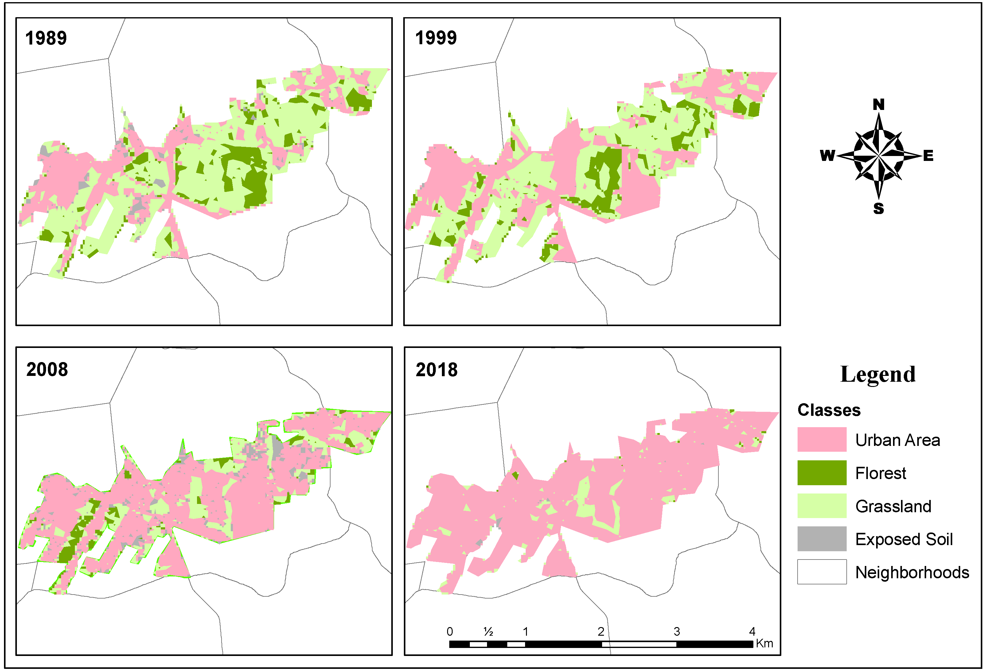
| Years | Urban Area | Grassland | Forest | Exposed Soil |
|---|---|---|---|---|
|
LST (°C)/Area (%) |
LST (°C)/Area (%) |
LST (°C)/Area (%) |
LST (°C)/Area (%) | |
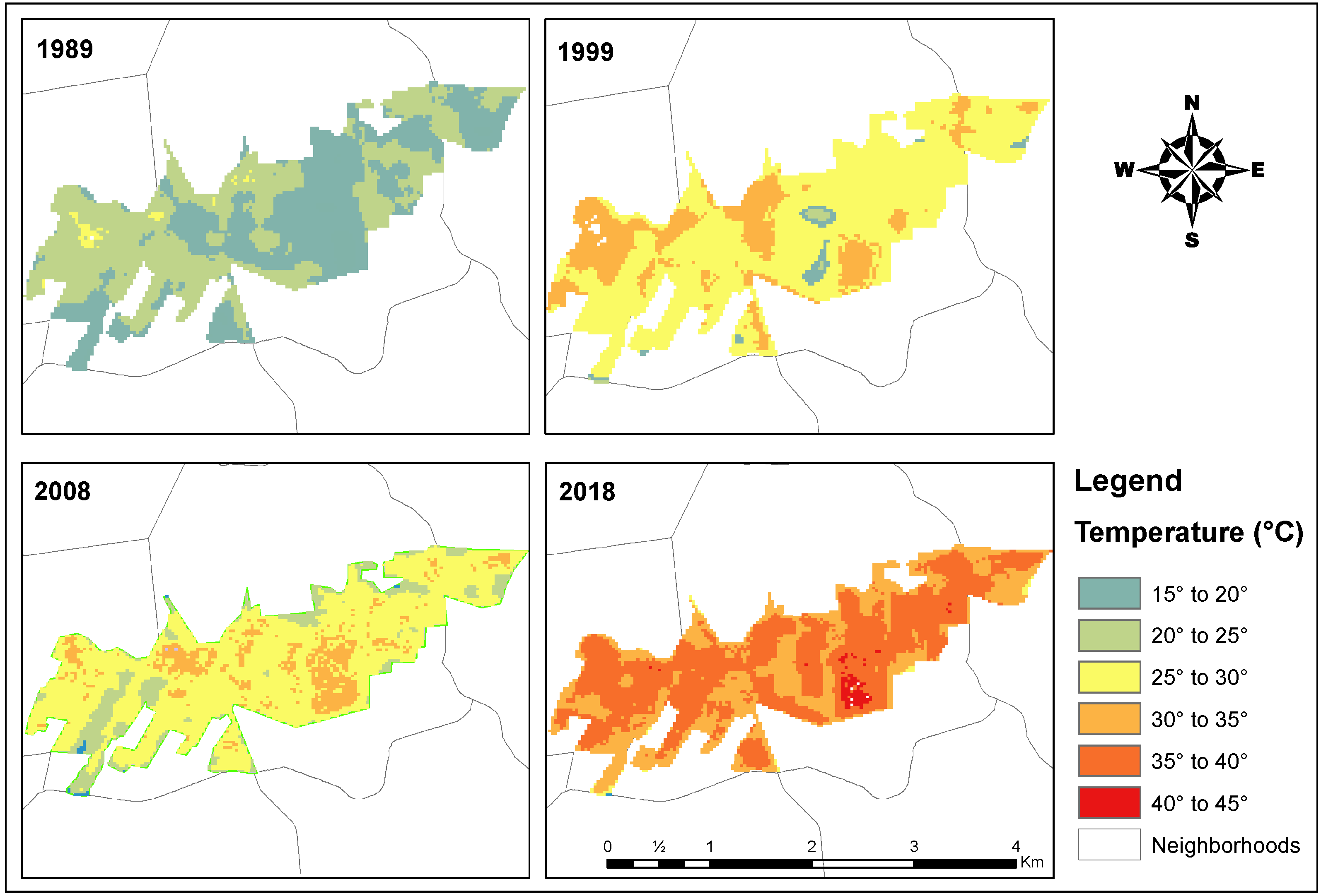
| 1989 | 22.5/31.0 | 20.8/51.0 | 18.9/14.4 | 22.6/03.6 |
| 1999 | 30.9/44.1 | 28.3/42.4 | 26.7/13.3 | 31.5/00.2 |
| 2008 | 29.2/65.6 | 26.9/19.9 | 24.7/05.6 | 28.3/08.9 |
| 2018 | 36.5/91.0 | 33.9/07.8 | 32.5/00.6 | 38.1/00.5 |
| Urban Area | Grassland | Forest | Exposed Soil | |
|---|---|---|---|---|
| Summer | 0.26 | −0.35 | −0.13 | 0.51 |
| Autumn | 0.49 | −0.50 | −0.26 | 0.12 |
| Winter | 0.25 | −0.16 | −0.32 | −0.06 |
| Spring | 0.25 | −0.20 | −0.16 | −0.04 |
| Intervals | Summer | Autmumn | Winter | Spring | ||||
|---|---|---|---|---|---|---|---|---|
| Mean | STD | Mean | STD | Mean | STD | Mean | STD | |
| 1989–1999 | 32.85 | 3.07 | 20.20 | 5.85 | 18.38 | 4.83 | 29.88 | 5.70 |
| 1999–2008 | 32.81 | 3.06 | 22.76 | 7.75 | 16.95 | 7.50 | 31.14 | 3.57 |
| 2008–2018 | 36.94 | 4.14 | 26.56 | 3.88 | 20.79 | 4.69 | 34.28 | 3.84 |
| Summer | Autumn | Winter | Spring | |
|---|---|---|---|---|
| Observations | 29 | 27 | 26 | 33 |
| Minimum | 27.85 | 12.64 | 9.74 | 18.88 |
| Maximum | 42.66 | 32.20 | 29.50 | 39.42 |
| Mean | 33.40 | 22.79 | 18.84 | 31.92 |
| Std. deviation | 3.41 | 5.92 | 5.33 | 4.84 |
| Kendall’s tau | 0.23 | 0.32 | 0.13 | 0.27 |
| S | 94 | 111 | 41 | 144 |
| p-value | 0.08 | 0.02 | 0.38 | 0.03 |
| Year | Urban Area | Grassland | Forest | Exposed Soil |
|---|---|---|---|---|
| 1989 | −0.55 | −0.03 | 0.12 | −0.40 |
| 1999 | −0.58 | −0.30 | −0.30 | −0.72 |
| 2008 | −0.59 | −0.39 | −0.07 | −0.56 |
| 2018 | −0.76 | −0.28 | −0.16 | −0.06 |
| Statistic | 1989 | 1999 | 2008 | 2018 |
|---|---|---|---|---|
| Mean LST (°C) | 21.10 | 29.25 | 28.43 | 36.42 |
| STD LST (°C) | 2.02 | 2.27 | 2.18 | 2.29 |
| Mean (NDVI) | 0.59 | 0.57 | 0.40 | 0.40 |
| STD (NDVI) | 0.15 | 0.21 | 0.19 | 0.18 |
| R (LST-NDVI) | −0.64 | −0.79 | −0.79 | −0.78 |
Publisher’s Note: MDPI stays neutral with regard to jurisdictional claims in published maps and institutional affiliations. |
© 2022 by the authors. Licensee MDPI, Basel, Switzerland. This article is an open access article distributed under the terms and conditions of the Creative Commons Attribution (CC BY) license (https://creativecommons.org/licenses/by/4.0/).
Share and Cite
Kaiser, E.A.; Rolim, S.B.A.; Grondona, A.E.B.; Hackmann, C.L.; de Marsillac Linn, R.; Käfer, P.S.; da Rocha, N.S.; Diaz, L.R. Spatiotemporal Influences of LULC Changes on Land Surface Temperature in Rapid Urbanization Area by Using Landsat-TM and TIRS Images. Atmosphere 2022, 13, 460. https://doi.org/10.3390/atmos13030460
Kaiser EA, Rolim SBA, Grondona AEB, Hackmann CL, de Marsillac Linn R, Käfer PS, da Rocha NS, Diaz LR. Spatiotemporal Influences of LULC Changes on Land Surface Temperature in Rapid Urbanization Area by Using Landsat-TM and TIRS Images. Atmosphere. 2022; 13(3):460. https://doi.org/10.3390/atmos13030460
Chicago/Turabian StyleKaiser, Eduardo Andre, Silvia Beatriz Alves Rolim, Atilio Efrain Bica Grondona, Cristiano Lima Hackmann, Rodrigo de Marsillac Linn, Pâmela Suélen Käfer, Nájila Souza da Rocha, and Lucas Ribeiro Diaz. 2022. "Spatiotemporal Influences of LULC Changes on Land Surface Temperature in Rapid Urbanization Area by Using Landsat-TM and TIRS Images" Atmosphere 13, no. 3: 460. https://doi.org/10.3390/atmos13030460