Analyzing the Characteristics of Cloud Condensation Nuclei (CCN) in Hebei, China Using Multi-Year Observation and Reanalysis Data

Abstract

The study of the characteristics and variations of cloud condensation nuclei (CCN) plays an important role in understanding the effects of aerosol–cloud interactions. This paper selected observation data in a city region of Shijiazhuang in North China from 2005 to 2007, along with the corresponding MERRA-2 and ERA5 data, to analyze the characteristics of CCN, sort the factors affecting the diurnal variation of CCN number concentration (${\mathrm{N}}_{\mathrm{CCN}}$) according to their importance, and build the relationship between ${\mathrm{N}}_{\mathrm{CCN}}$ and supersaturation ($\mathrm{SS}$) in the heavily polluted region. The results show that there was a bimodal distribution of a daily time series for ${\mathrm{N}}_{\mathrm{CCN}}$ in Shijiazhuang, China. By calculating the correlation between CCN and pollutants observed in winter 2007, we identified that the dominant factor for peaks of ${\mathrm{N}}_{\mathrm{CCN}}$ is ${\mathrm{SO}}_2$ in the morning but ${\mathrm{NO}}_2$ in the evening. We also ranked the factors affecting the diurnal variation of ${\mathrm{N}}_{\mathrm{CCN}}$ by using observation and reanalysis data and found that the concentration of pollutants is the greatest impact factor in summer, but the atmospheric stability is the greatest factor in winter. Finally, we determined the relationship between ${\mathrm{N}}_{\mathrm{CCN}}$ and $\mathrm{SS}$ according to the Twomey formula (${\mathrm{N}}_{\mathrm{CCN}}={\mathrm{cSS}}^{\mathrm{k}}$) and found there was a reasonable value range (i.e., 0.5~0.7) for the parameter $\mathrm{k}$ in East and North China. Specifically, it is more reasonable for $\mathrm{k}$ to be 0.5 in summer and 0.7 in winter.

1. Introduction

The multiphase system composed of solid and liquid particles suspended in the air is called aerosol. Changes in aerosol composition, particle size, and number concentration have important effects on the radiation budget, clouds, and precipitation in the earth system [1,2,3,4]. Aerosols can cool (and warm) the earth–atmosphere system by scattering (absorbing) solar radiation directly (i.e., aerosol–radiation interaction). In addition, a part of aerosols can also indirectly affect cloud radiative properties [2] and precipitation processes [5] by influencing the cloud droplet size/number of warm stratus clouds, namely aerosol–cloud interaction. These aerosols are called cloud condensation nuclei (CCN). CCN plays a significant role in aerosol and cloud physics as it links aerosol characteristics to the cloud formation process. Due to the complexity of aerosol–cloud interaction and cloud/rain processes, there are large uncertainties in estimating the effect of aerosol on climate using global climate models (GCM) [6,7,8]. To better evaluate climate model simulation on aerosol–cloud interaction and reduce the uncertainty, it is necessary to conduct a more in-depth study on the characteristics of CCN over large-scale and long-term spatial-temporal domains.

The number concentration of CCN (${\mathrm{N}}_{\mathrm{CCN}}$, ${\mathrm{cm}}^{-3}$) has a large spatial variability. For example, in the case of 1% supersaturation ($\mathrm{SS}$), the clean region usually has ${\mathrm{N}}_{\mathrm{CCN}}<1000$, the polluted region has $1000 \le {\mathrm{N}}_{\mathrm{CCN}}<10,000$, and the heavily polluted region even shows ${\mathrm{N}}_{\mathrm{CCN}} \ge 10,000$. It is relatively common to carry out studies in clean or polluted regions, such as New York (${\mathrm{N}}_{\mathrm{CCN}}<3000$ at $\mathrm{SS}=1\%$, similarly hereinafter) [9], Helsinki (${\mathrm{N}}_{\mathrm{CCN}}<1500$) [10], Shanghai (${\mathrm{N}}_{\mathrm{CCN}}<8500$) [11], Azores (${\mathrm{N}}_{\mathrm{CCN}}<300$) [12], and Seoul (${\mathrm{N}}_{\mathrm{CCN}}<10,000$) [13]. Alternatively, few observations were carried out in heavily polluted regions, such as India (${\mathrm{N}}_{\mathrm{CCN}}$ at $\mathrm{SS}=0.6\%$ up to 25,000) or the North China Plain and Yangtze River Delta in China ($13,000\le {\mathrm{N}}_{\mathrm{CCN}}<30,000$) [14,15,16,17,18,19]. Fewer observations lead to a lack of thorough understanding of the characteristics of CCN in heavily polluted regions. Meanwhile, lacking long-term observational data is another reason for restricting the research of CCN characteristics in heavily polluted regions. Previous studies usually focused on a short-term variation of CCN due to the limitation of observational conditions. Most studies had an effective time of observation for less than one year [10,11,12,16,17,18,19,20,21,22,23,24,25,26,27,28,29,30], some for one season [16,18,19,21,26,30] and even for several days [17,24,25,28,29]. Although some studies have been carried out using long-term observations located at some representative areas [13,31,32,33,34], most of them are in clean or polluted areas where biomass burning is the main source of pollution [32,33,34], and the observations sampled on high-polluting areas affected by human activities are relatively rare [13,31]. Short-term data have limited representativeness and are not applicable for evaluation on large-scale simulations with GCM. Therefore, it is essential to carry out a long-term CCN observation for better characterizing CCN in heavily polluted regions.

${\mathrm{N}}_{\mathrm{CCN}}$ has obvious diurnal changes, and usually shows a unimodal or bimodal distribution. Although many studies on CCN pointed out this pattern and gave some qualitative analyses, such as boundary layer height ($\mathrm{BLH}$) [13,19,21,25,27,28,29], pollutant emissions [11,13,16,17,18,19,21,24,25,26,27,28,29,30], aerosol types [10,12,21,27], and photochemical processes [11,13,24,25,27], the quantitative analyses of influencing factors are rare. Taking $\mathrm{BLH}$ as an example, only Kim et al. [13] and Wang et al. [18] in the above studies used the micro-pulse lidar data for qualitative verification, and others just analyzed the theoretical feasibility. This is largely limited by the lack of observational data. At present, reanalysis data have been widely used in climate studies [35,36,37,38], and it is feasible to combine the reanalysis data with long-term CCN observation to analyze the influencing factors and their respective impacts on ${\mathrm{N}}_{\mathrm{CCN}}$ variations.

In addition, the parameterization of ${\mathrm{N}}_{\mathrm{CCN}}$ is also a focus of previous research. The Twomey formula is one of the most widely used parameterizations for determining ${\mathrm{N}}_{\mathrm{CCN}}$ through $\mathrm{SS}$, namely, ${\mathrm{N}}_{\mathrm{CCN}}={\mathrm{cSS}}^{\mathrm{k}}$ [39]. Therefore, the determination of $\mathrm{c}$ and $\mathrm{k}$ in this parameterization scheme is an important objective as well. Some studies fitted parameters for a certain season by using single-year observation data. For example, Hudson [40] and Martins et al. [41] determined the parameters of autumn in America and Brazil, respectively. More generally, however, researchers could only obtain parameters for a short-term period (typically for days) because of the limitation of data, especially in China [18,24,25,27,29]. The lack of the parameterization scheme derived from long-term CCN data hinders the further application in GCM and large-scale studies.

Beginning in the 11th FYP (Five-Year Plan) in 2006–2010, the Chinese government set a goal of controlling air pollution and put efforts in reducing the sulfate emissions from coal combustion by utilizing new techniques of desulfurization. In September 2013, the “Air Pollution Prevention and Control Action Plan” was released and became the most influential policy for improving China’s environment in the subsequent decade. Correspondingly, the air quality in North China has been continuously improved since 2010, as shown from multiple surface measurements [42,43] or satellite datasets [44,45]. Therefore, we left out the CCN data after 2010 as our study focused on CCN in the heavily polluted period. Noting that 2006 was a year with severe pollution [46], the observation data from 2005 to 2007 were therefore selected for application in this study.

This paper selected multi-season measurements conducted in Shijiazhuang, a polluted megacity, and used the observations in summer and winter during 2005–2007 to analyze the characteristics of CCN. The concurrent data, which includes the Modern-Era Retrospective Analysis for Research and Applications version 2 (MERRA-2) and the ECMWF Reanalysis 5th Generation (ERA5), are also analyzed to identify the factors affecting the diurnal variation of ${\mathrm{N}}_{\mathrm{CCN}}$, and build the relationship between ${\mathrm{N}}_{\mathrm{CCN}}$ and $\mathrm{SS}$ in the heavily polluted region. This paper is organized as follows. The next section describes the data and methodology, followed by the results illustrated in Section 3. The conclusion and discussion are given in Section 4.

2. Data and Methodology

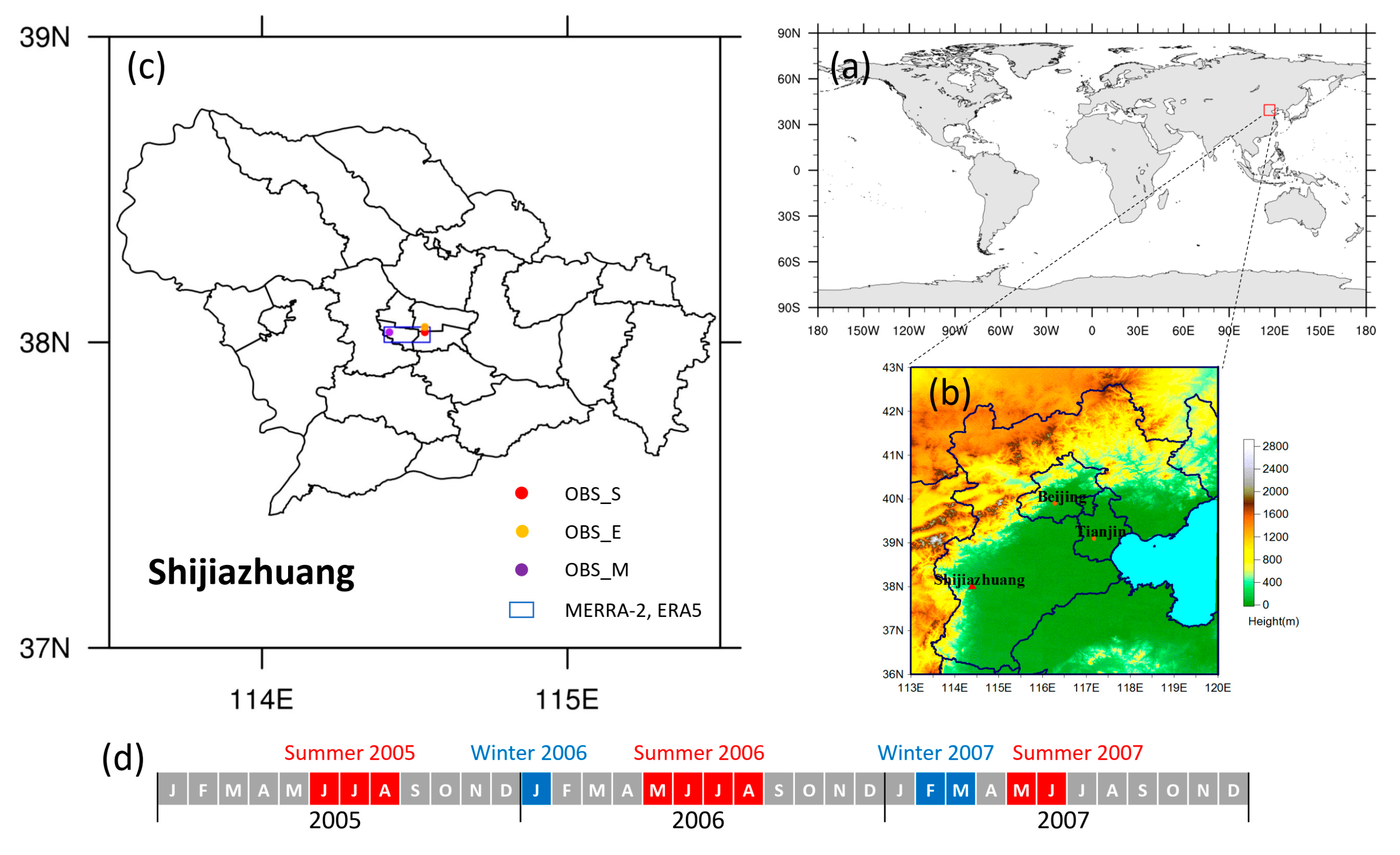
2.1. Station Data

Shijiazhuang (38°02′ N, 114°31′ E), the capital of Hebei, China, was selected as the studying site, which is a megacity in North China and located at one of the polluted regions in the world [47]. Here, we utilized the following observed data, including the concentrations of CCN, pollutants (${\mathrm{PM}}_{10}$, ${\mathrm{NO}}_2$ and ${\mathrm{SO}}_2$), and meteorological variables (temperature and wind speed), to study the characteristics of CCN in the heavily polluted region. The location of the study area and the observed periods are shown in Figure 1. CCN was observed at the Hebei Meteorological Service Station (38°02′ N, 114°32′ E) (OBS_S for short) from 2005 to 2007 (see all the CCN measurement periods in the caption of

Table 1. The detailed information for variables used in this study.

Variable	Description	Unit	Data Source	Time
${\mathrm{M}}_{\mathrm{PM}10}$	$\mathrm{Mass}\mathrm{concentration}\mathrm{of}{\mathrm{PM}}_{10}$	${\mathsf{\mu }\mathrm{g}\mathrm{m}}^{-3}$	OBS_E	28 February 2007–12 March 2007 (winter 2007)
${\mathrm{M}}_{\mathrm{SO}2}$	$\mathrm{Mass}\mathrm{concentration}\mathrm{of}{\mathrm{SO}}_2$	${\mathsf{\mu }\mathrm{g}\mathrm{m}}^{-3}$	OBS_E
${\mathrm{M}}_{\mathrm{NO}2}$	$\mathrm{Mass}\mathrm{concentration}\mathrm{of}{\mathrm{NO}}_2$	${\mathsf{\mu }\mathrm{g}\mathrm{m}}^{-3}$	OBS_E
${\mathrm{N}}_{\mathrm{CCN}}$	The number concentration of CCN	${\mathrm{cm}}^{-3}$	OBS_S	24 June 2005–9 August 2005 (summer 2005), 1 January 2006–19 January 2006 (winter 2006) 21 May 2006–19 August 2006 (summer 2006), 28 February 2007–12 March 2007 (winter 2007), and 24 May 2007–30 June 2007 (summer 2007)
${\mathrm{M}}_{\mathrm{Dust}}$	Surface mass concentration of dust	${\mathrm{kg}\mathrm{m}}^{-3}$	MERRA-2
${\mathrm{C}}_{\mathrm{SO}2}$	$\mathrm{Column}\mathrm{mass}\mathrm{concentration}\mathrm{of}{\mathrm{SO}}_2$	${\mathrm{kg}\mathrm{m}}^{-2}$	MERRA-2
${\mathrm{C}}_{\mathrm{O}3}$	Total column concentration of ozone	DU	MERRA-2
${\mathrm{C}}_{\mathrm{BC}}$	Column mass concentration of black carbon	${\mathrm{kg}\mathrm{m}}^{-2}$	MERRA-2
${\mathrm{T}}_{\mathrm{M}}$	Temperature	K	MERRA-2,
${\mathrm{T}}_{\mathrm{O}}$	Temperature	K	OBS-M,
${\mathrm{T}}_{\mathrm{E}}$	Temperature	K	ERA5
$\mathrm{WS}{10}_{\mathrm{M}}$	10 m wind speed	${\mathrm{m}\mathrm{s}}^{-1}$	MERRA-2,
$\mathrm{WS}{10}_{\mathrm{O}}$	10 m wind speed	${\mathrm{m}\mathrm{s}}^{-1}$	OBS-M,
$\mathrm{WS}{10}_{\mathrm{E}}$	10 m wind speed	${\mathrm{m}\mathrm{s}}^{-1}$	ERA5
$\mathrm{RH}$	Relative humidity	%	ERA5
$\mathrm{WS}$	Surface wind speed	${\mathrm{m}\mathrm{s}}^{-1}$	MERRA-2
$\mathrm{BLH}$	Boundary layer height	m	ERA5
$\mathrm{BLD}$	Boundary layer dissipation	${\mathrm{J}\mathrm{m}}^{-2}$	ERA5
$\mathrm{CAPE}$	Convective available potential energy	${\mathrm{J}\mathrm{kg}}^{-1}$	ERA5
$\mathrm{CIN}$	Convective inhibition	${\mathrm{J}\mathrm{kg}}^{-1}$	ERA5

). The observation site of pollutants was located at the Environmental Monitoring Center (38°03′ N, 114°32′ E) (OBS_E) and was about 3 km away from the OBS_S, where the mass concentrations of ${\mathrm{PM}}_{10}$, ${\mathrm{NO}}_2$ and ${\mathrm{SO}}_2$ were measured from 28 February 2007–12 March 2007. To facilitate comparative analysis, we divided all sampling periods by season (panel d in Figure 1 or column “Time” in Table 1), where “winter” and “summer” are roughly defined as in the period of “December–January–February” and “June–July–August”, respectively, and allowing a half-month extension of the period for including as much data as possible. Meteorological data were obtained in the Meteorological Observation Station (38°02′ N, 114°25′ E) (OBS_M), approximately 9 km away from the OBS_S station, where surface temperature and wind speed at 10 m height were available during all the CCN measurement periods.

In the OBS_S site, a CCN Counter, model CCN-100 from Droplet Measurement Technologies (DMT; Boulder, CO, USA), was used to measure the ${\mathrm{N}}_{\mathrm{CCN}}$ at 4 different $\mathrm{SS}$ levels (0.1%, 0.3%, 0.5% and 1.0%) by utilizing the difference between the heat and moisture diffusion coefficients [48]. The theoretical error of CCN concentration observed by this CCN Counter is no more than 10% [49]. To ensure the accuracy of the CCN data, the CCN Counter was calibrated by the manufacturers every year before observations [14]. The CCN data have a temporal resolution of 1 s and were processed by hourly averaging before analysis. In the OBS_E and OBS_M sites, pollutants (e.g., the mass concentrations of ${\mathrm{PM}}_{10}$ (${\mathrm{M}}_{\mathrm{PM}10}$), ${\mathrm{NO}}_2$ (${\mathrm{M}}_{\mathrm{NO}2}$) and ${\mathrm{SO}}_2$ (${\mathrm{M}}_{\mathrm{SO}2}$)) and meteorological elements (the surface temperature (${\mathrm{T}}_{\mathrm{O}}$) and 10 m wind speed ($\mathrm{WS}{10}_{\mathrm{O}}$)) data were provided, respectively. Both of them have a temporal resolution of 1 h. See Table 1 for more details.

2.2. Reanalysis Data

To analyze the factors affecting the long-term CCN variation more comprehensively, we needed corresponding climatological data to assist. Here, MERRA-2 and ERA5 data of Shijiazhuang region (38°00′ N–38°03′ N, 114°24′ E–114°33′ E) were extracted. MERRA-2 is the latest atmospheric reanalysis of the modern satellite era produced by NASA’s Global Modeling and Assimilation Office (GMAO) [50], which was often used to analyze aerosol characteristics and aerosol-climate interaction and relations [51,52,53]. MERRA-2 data have been proved to be reliable in representing the long-term temporal and spatial distribution of pollutants (i.e., ${\mathrm{PM}}_{2.5}$, ${\mathrm{PM}}_{10}$ sulfate, organic carbon, and black carbon) in China [54,55,56]. We downloaded the pollutants and meteorological data from Giovanni (https://giovanni.gsfc.nasa.gov/giovanni/, accessed on 21 January 2020), including the data of surface mass concentration of dust (${\mathrm{M}}_{\mathrm{Dust}}$), the column mass concentration of ${\mathrm{SO}}_2$ (${\mathrm{C}}_{\mathrm{SO}2}$), the total column concentration of ozone (${\mathrm{C}}_{\mathrm{O}3}$), the column mass concentration of black carbon (${\mathrm{C}}_{\mathrm{BC}}$), the surface temperature (${\mathrm{T}}_{\mathrm{M}}$), the 10-m wind speed ($\mathrm{WS}{10}_{\mathrm{M}}$), and the surface wind speed ($\mathrm{WS}$). ERA5 performs decently in characterizing meteorological conditions (i.e., temperature, wind speed, and precipitation) for climate studies [57,58]. Therefore, ERA5 data (https://cds.climate.copernicus.eu/cdsapp#!/home, accessed on 8 January 2020) were used to analyze the effect of meteorological conditions on CCN variation in this study, we extracted the data of surface temperature (${\mathrm{T}}_{\mathrm{E}}$), the relative humidity ($\mathrm{RH}$), the 10-m wind speed ($\mathrm{WS}{10}_{\mathrm{E}}$), the boundary layer height ($\mathrm{BLH}$), the boundary layer dissipation ($\mathrm{BLD}$), the convective available potential energy ($\mathrm{CAPE}$), and the convective inhibition ($\mathrm{CIN})$. Both MERRA-2 and ERA5 data are processed as hourly data, and more information about them had shown in Table 1.

2.3. Methodology

We verified the consistency between MERRA-2 and ERA5 data with available observational data at the OBS-M site, e.g., $\mathrm{WS}{10}_{\mathrm{O}}$ for verifying 10 m wind speeds $\mathrm{WS}{10}_{\mathrm{M}}$ and $\mathrm{WS}{10}_{\mathrm{E}}$, and ${\mathrm{T}}_{\mathrm{O}}$ for verifying surface temperature ${\mathrm{T}}_{\mathrm{M}}$ and ${\mathrm{T}}_{\mathrm{E}}$. The result showed that the Pearson correlation coefficient ($\mathrm{r}$) values of $\mathrm{WS}{10}_{\mathrm{M}}$ and $\mathrm{WS}{10}_{\mathrm{E}}$ with $\mathrm{WS}{10}_{\mathrm{O}}$ are 0.677 and 0.591, respectively. For the temperature, the $\mathrm{r}$ values are 0.963 and 0.940, respectively. All results passed the consistency test with a 95% confidence level, indicating a reasonable consistency between the reanalysis data and the observations. Therefore, we used both MERRA-2 and ERA5 data to carry out analyses when the station data were not available.

To highlight the variation of each variable, we mainly used the normalized changes of a variable, as defined below:

$$\mathrm{V}=\frac{{\mathrm{V}}_{\mathrm{t}}-{\mathrm{V}}_{\mathrm{MIN}}}{{\mathrm{V}}_{\mathrm{MAX}}-{\mathrm{V}}_{\mathrm{MIN}}}$$

(1)

where $\mathrm{V}$ (V can be any individual variable normalized in a specified period in Table 1, e.g., ${\mathrm{N}}_{\mathrm{CCN}}$ in winter 2007) means the time series of the normalized change of ${\mathrm{V}}_{\mathrm{t}}$, which is the value of a variable at a certain observational time point $\mathrm{t}$ (e.g., measured ${\mathrm{N}}_{\mathrm{CCN}}$ at one day in winter 2007), and ${\mathrm{V}}_{\mathrm{MAX}}$ and ${\mathrm{V}}_{\mathrm{MIN}}$ represent the maximum and minimum values of the variable during the whole observational period (e.g., maximum and minimum values of ${\mathrm{N}}_{\mathrm{CCN}}$ in winter 2007). The time series of normalized data can highlight the relative variations of variables, reduce the complexity of graphics, and avoid the dimensional conversion, making our analysis process more concise.

We used the Pearson correlation coefficient ($\mathrm{r}$) to characterize the correlation (linear correlation) between different variables [59]. It is worthy of noting that the use of the normalized method does not change the $\mathrm{r}$ values between different variables, ensuring the reliability of our correlation analysis.

3. Results

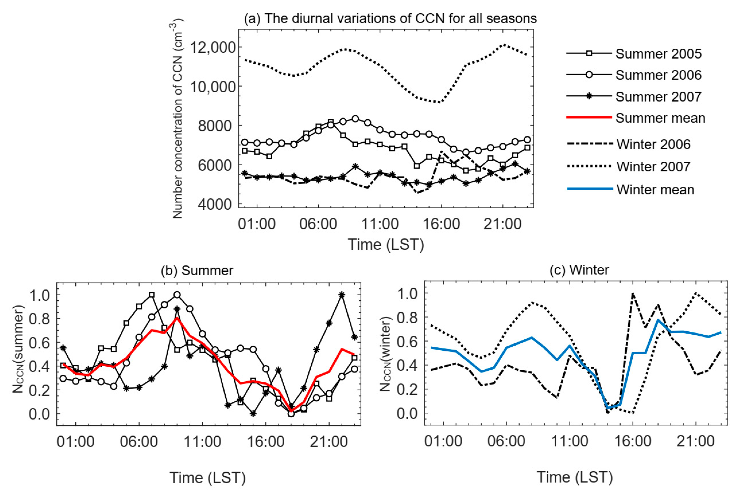
3.1. Diurnal Variation of N_CCN

Considering the ${\mathrm{N}}_{\mathrm{CCN}}$ data with $\mathrm{SS}=0.3 \%$ had more valid data samples, we selected the ${\mathrm{N}}_{\mathrm{CCN}}$ under this supersaturation to analyze the characteristics of diurnal variation. The absolute variations of ${\mathrm{N}}_{\mathrm{CCN}}$ in five measurement periods are shown in Figure 2a. In addition, to highlight the characteristics of the diurnal variation, the normalized ${\mathrm{N}}_{\mathrm{CCN}}$ in summer and winter are plotted in Figure 2b,c. Overall, the diurnal variations of ${\mathrm{N}}_{\mathrm{CCN}}$ in different periods show bimodal distributions. In detail, there are some differences in ${\mathrm{N}}_{\mathrm{CCN}}$ daily series between winter and summer. On one hand, the intensities of the two peaks are not consistent. The peak in the morning is more prominent for summer, but the peak in the evening is stronger for winter. On the other hand, the times hitting peak points in different seasons are also different. In summer, the double peaks appear around 09:00 Local Standard Time (LST) in the morning and 22:00 LST in the evening, whereas the peaks appear around 08:00 LST in the morning and 18:00 LST in the evening in winter. The above results show that the diurnal variations of ${\mathrm{N}}_{\mathrm{CCN}}$ in winter and summer might be influenced by different factors. We analyze the possible influencing factors in more detail in Section 3.3.

3.2. Diurnal Variation of N_CCN in Winter

Pollutants in the atmosphere have an important effect on the aerosol ability for activating to form cloud droplets. Zhang et al. [60] pointed out that aerosol activity is linked not only to particle composition but also to mixing state, aging, and physical processes (such as coating and condensation). The impact of highly soluble pollutants, such as gas precursors such as ${\mathrm{SO}}_2$ and ${\mathrm{NO}}_2$, can affect the formation of hygroscopic matter, and influence particle hygroscopicity [61]. The more ${\mathrm{SO}}_2$ and ${\mathrm{NO}}_2$ coating in the aerosol, the more hygroscopic the particles are and the easier the particles to serve as CCN. Here, we obtained the hourly-averaged concentrations of pollutants (${\mathrm{NO}}_2$, ${\mathrm{PM}}_{10}$ and ${\mathrm{SO}}_2$) from the available station data in winter 2007 and made use of them to identify the possible reasons for the two peaks occurring in the diurnal variations of ${\mathrm{N}}_{\mathrm{CCN}}$. As shown in Figure 3, ${\mathrm{N}}_{\mathrm{CCN}}$ is highly consistent with the concentrations of pollutants, especially for ${\mathrm{NO}}_2$ and ${\mathrm{PM}}_{10}$. The $\mathrm{r}$ values of ${\mathrm{M}}_{\mathrm{NO}2}$ and ${\mathrm{M}}_{\mathrm{PM}10}$ with ${\mathrm{N}}_{\mathrm{CCN}}$ are 0.789 and 0.771, and all pass the consistency test with a confidence of 99%. In terms of a.m. and p.m. periods, the positive relationship is apparent for ${\mathrm{SO}}_2$ ($\mathrm{r}=0.797$) at a.m., and for ${\mathrm{NO}}_2$ ($\mathrm{r}=0.933$) at p.m., suggesting that the dominant factor affecting the diurnal variation of ${\mathrm{N}}_{\mathrm{CCN}}$ is time-dependent. In the morning, ${\mathrm{SO}}_2$ plays a critical role, but the role of ${\mathrm{NO}}_2$ is more significant in the afternoon and becomes a dominant factor in the evening. ${\mathrm{PM}}_{10}$ and ${\mathrm{N}}_{\mathrm{CCN}}$ always maintain a high positive correlation all day, which indicates that the total aerosol particle concentration plays a decisive role in the ${\mathrm{N}}_{\mathrm{CCN}}$ variation. Note that the data analyzed in this sub-section only reflect winter 2007. The pollutant of ${\mathrm{SO}}_2$ is mainly emitted from the heating facilities in North China [62,63], and the frequently occurring temperature inversion in winter evenings may accumulate the pollutant to reach a peak in the morning. The pollutant of ${\mathrm{NO}}_2$ is mainly from the traffic emission in the daytime [64], and likely accumulates to reach a peak in the evening.

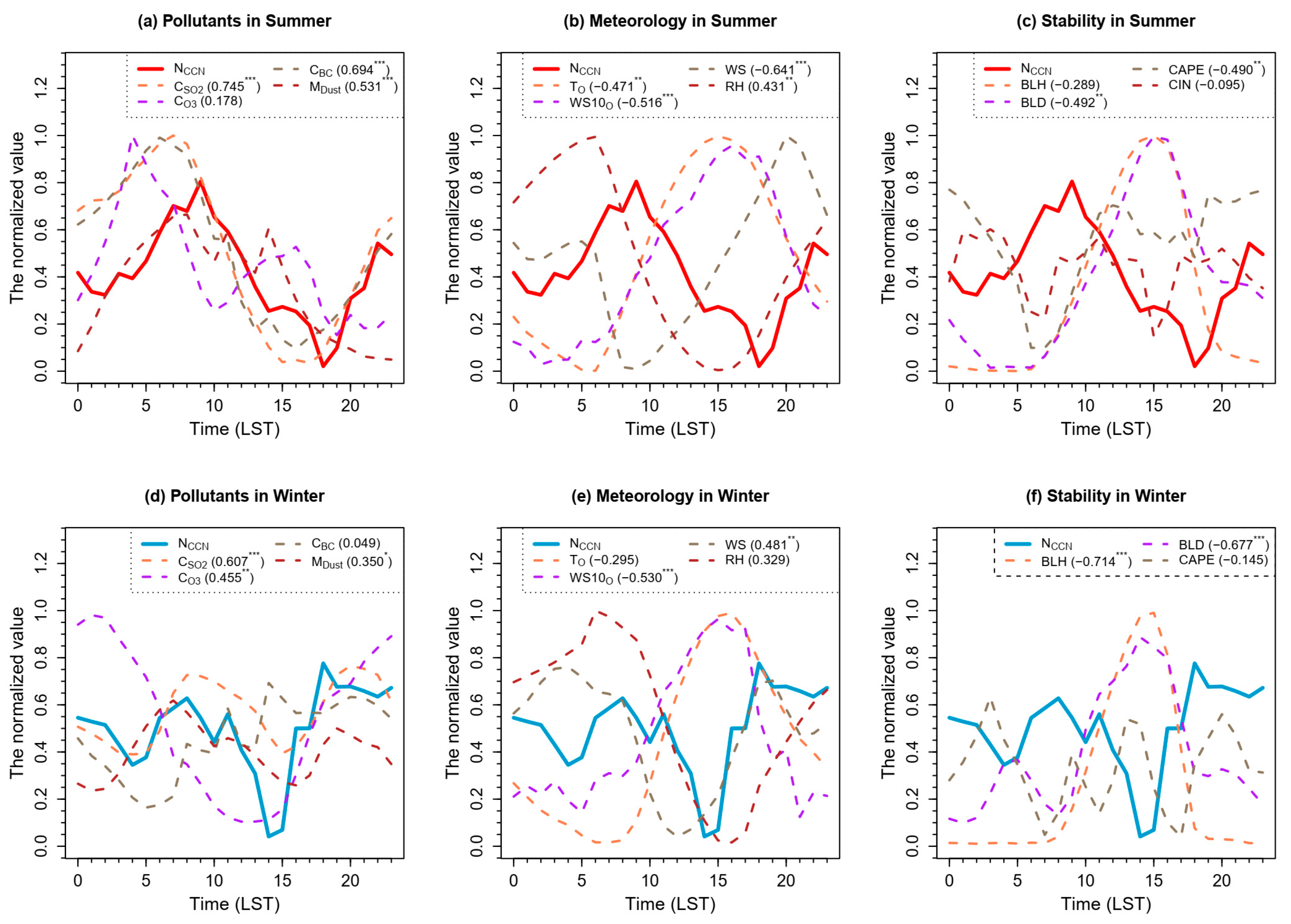
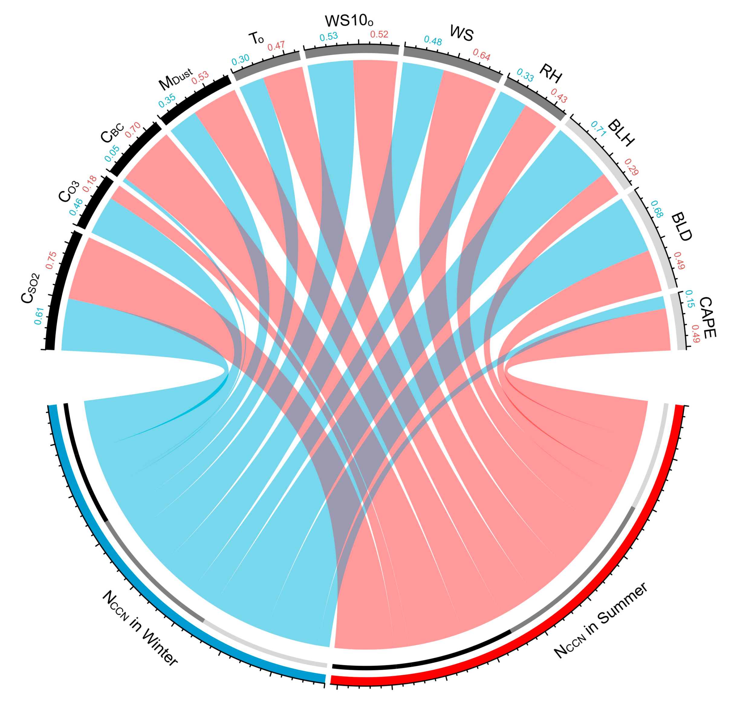
3.3. Factors Affecting the Diurnal Variation of N_CCN

The diurnal variations of ${\mathrm{N}}_{\mathrm{CCN}}$ are related to the factors affecting the aerosol activation, for instance, the physical and chemical characteristics of the aerosol, and the meteorological conditions. To quantify the effects of these factors, we plotted their variations and calculated the correlation $\mathrm{r}$ between ${\mathrm{N}}_{\mathrm{CCN}}$ and the following variables: pollutants (${\mathrm{C}}_{\mathrm{SO}2}$,${\mathrm{C}}_{\mathrm{O}3}$, ${\mathrm{C}}_{\mathrm{BC}}$, and ${\mathrm{M}}_{\mathrm{Dust}}$), meteorological variables (${\mathrm{T}}_{\mathrm{O}}$,$\mathrm{WS}{10}_{\mathrm{O}}$, $\mathrm{WS}$ and $\mathrm{RH}$), and atmospheric stability variables ($\mathrm{BLH}$,$\mathrm{BLD}$,$\mathrm{CAPE}$, and $\mathrm{CIN}$), as shown in Figure 4 and

Table 2. The importance ranking of the factors affecting ${\mathrm{N}}_{\mathrm{CCN}}$ diurnal variation according to the absolute value of correlation $\mathrm{r}$ for summer and winter during 2005–2007. Results that pass the 90% confidence test are indicated in bold. The superscripts of ***, **, and * present the correlations passing the consistency test with the significance levels of 99%, 95% and 90%, respectively.

Order	Summer			Winter
	Variable	r	p-Value	Variable	r	p-Value
1	${\mathrm{C}}_{\mathrm{SO}2}$	0.745 ***	0.00003	$\mathrm{BLH}$	−0.714 ***	0.00009
2	${\mathrm{C}}_{\mathrm{BC}}$	0.694 ***	0.00017	$\mathrm{BLD}$	−0.677 ***	0.00028
3	$\mathrm{WS}$	−0.641 ***	0.00073	${\mathrm{C}}_{\mathrm{SO}2}$	0.607 ***	0.00166
4	${\mathrm{M}}_{\mathrm{Dust}}$	0.531 ***	0.00761	$\mathrm{WS}{10}_{\mathrm{O}}$	−0.530 ***	0.00778
5	$\mathrm{WS}{10}_{\mathrm{O}}$	−0.516 ***	0.00984	$\mathrm{WS}$	0.481 **	0.01725
6	$\mathrm{BLD}$	−0.492 **	0.01456	${\mathrm{C}}_{\mathrm{O}3}$	0.455 **	0.02559
7	$\mathrm{CAPE}$	−0.490 **	0.01504	${\mathrm{M}}_{\mathrm{Dust}}$	0.350 *	0.09329
8	${\mathrm{T}}_{\mathrm{O}}$	−0.471 **	0.02008	$\mathrm{RH}$	0.329	0.11667
9	$\mathrm{RH}$	0.431 **	0.03543	${\mathrm{T}}_{\mathrm{O}}$	−0.295	0.16123
10	$\mathrm{BLH}$	−0.289	0.17083	$\mathrm{CAPE}$	−0.145	0.49900
11	${\mathrm{C}}_{\mathrm{O}3}$	0.178	0.40573	${\mathrm{C}}_{\mathrm{BC}}$	0.049	0.82153
12	$\mathrm{CIN}$	−0.095	0.65769	$\mathrm{CIN}$	--	--

. Here, pollutant and atmospheric stability data were sourced from the MERRA-2 and ERA5, respectively, and meteorological data were obtained from on-site observation and reanalysis data. The atmospheric stability variables are used to represent the environmental conditions for pollutants (emitted from the Earth’s surface) to diffuse away from the emission sources. $\mathrm{BLH}$ and $\mathrm{BLD}$ characterize the atmospheric state under tiny turbulence, and $\mathrm{CAPE}$ and $\mathrm{CIN}$ correspond to stronger atmospheric disturbances (i.e., convection). Note that $\mathrm{CIN}$ values are available only in summer. In general, pollutants will be diffused and the concentration near the source region will be diluted with high $\mathrm{BLH}$, $\mathrm{BLD}$, $\mathrm{CAPE},$ and low $\mathrm{CIN}$.

The hourly-averaged time series of different variables and ${\mathrm{N}}_{\mathrm{CCN}}$ in winter and summer are shown in Figure 4. In summer, the diurnal variation of pollutants and ${\mathrm{N}}_{\mathrm{CCN}}$ has a positive correlation. Among them, ${\mathrm{SO}}_2$ has the best correlation, followed by $\mathrm{BC}$ and dust, and finally ${\mathrm{O}}_3$ (Figure 4a). In terms of meteorological variables, temperature and wind speed are negatively correlated while $\mathrm{RH}$ is positively correlated to ${\mathrm{N}}_{\mathrm{CCN}}$. Wind speed (surface and 10 m wind speed) has the strongest correlation, followed by surface temperature and $\mathrm{RH}$ (Figure 4b). All atmospheric stability variables have a negative correlation with ${\mathrm{N}}_{\mathrm{CCN}}$ in the diurnal variation, of which the strongest correlation is $\mathrm{BLD},$ followed by $\mathrm{CAPE}$, and finally $\mathrm{BLH}$ and $\mathrm{CIN}$ (Figure 4c). In winter, the positive and negative correlations between different variables and ${\mathrm{N}}_{\mathrm{CCN}}$ in the diurnal variation are generally consistent with those in summer, but the strength of the correlation (i.e., $\mathrm{r}$) is different. For the pollutants, the diurnal variation of ${\mathrm{SO}}_2$ still has the strongest impact on ${\mathrm{N}}_{\mathrm{CCN}}$, followed by ${\mathrm{O}}_3$ and dust, and the least impacting pollutant is $\mathrm{BC}$ (Figure 4d). Wind speed is still the most important factor affecting ${\mathrm{N}}_{\mathrm{CCN}}$ among meteorological variables (Figure 4e). However, the correlation between surface wind speed and ${\mathrm{N}}_{\mathrm{CCN}}$ is negative in summer but positive in winter, which will be discussed later. There are strong negative correlation relationships between ${\mathrm{N}}_{\mathrm{CCN}}$ and atmospheric stability variables, especially for $\mathrm{BLH}$ and $\mathrm{BLD}$ (Figure 4f).

As mentioned above, $\mathrm{WS}{10}_{\mathrm{O}}$ (wind speed at 10 m height) and ${\mathrm{N}}_{\mathrm{CCN}}$ always show a negative correlation, but $\mathrm{WS}$ (surface wind speed) and ${\mathrm{N}}_{\mathrm{CCN}}$ have different correlations in different seasons. We explain the phenomenon as follows. Wind speed is regarded as an important factor affecting the source and sink of aerosol and pollutants. $\mathrm{WS}{10}_{\mathrm{O}}$ is higher from the ground and is mostly determined by the synoptic meteorology or the large-scale air circulation. The larger $\mathrm{WS}{10}_{\mathrm{O}}$ usually indicates stronger horizontal air motions and favors the diffusion of pollutants, resulting in a lower ${\mathrm{N}}_{\mathrm{CCN}}$. However, $\mathrm{WS}$ is strongly affected by the surface properties such as vegetation types, soil grains, surface roughness, etc., and is most likely determined by the local topography, and small- to middle-scale weather situations. Therefore, the relationship between $\mathrm{WS}$ and ${\mathrm{N}}_{\mathrm{CCN}}$ is prone to change with seasons.

To analyze the main influencing factors of ${\mathrm{N}}_{\mathrm{CCN}}$ in winter and summer, we sorted the variables according to the absolute values of $\mathrm{r}$, as shown in Figure 5. In this chord diagram, the absolute values of $\mathrm{r}$ denote the correlations between the corresponding variables and ${\mathrm{N}}_{\mathrm{CCN}}$ connected by the belt. The wider belt indicates the stronger correlation between the individual variable and ${\mathrm{N}}_{\mathrm{CCN}}$. For all the variables listed in Table 2, only those variables with correlations passing the test of 90% confidence level (i.e., p-value is less than 0.1) were selected to show in Figure 5. In summer, we see the variations in pollutants of ${\mathrm{C}}_{\mathrm{SO}2}$ and ${\mathrm{C}}_{\mathrm{BC}}$ have the greatest impact on that in ${\mathrm{N}}_{\mathrm{CCN}}$, followed by meteorological conditions of wind speed ($\mathrm{WS}$ and $\mathrm{WS}{10}_{\mathrm{O}}$), and finally atmospheric stability of $\mathrm{BLD}$ and $\mathrm{CAPE}$. In winter, the factor that has the greatest impact on ${\mathrm{N}}_{\mathrm{CCN}}$ variation is atmospheric stability of $\mathrm{BLH}$ and $\mathrm{BLD}$, followed by the pollutant of ${\mathrm{C}}_{\mathrm{SO}2}$, and the relatively minor factor is the meteorological condition of wind speed ($\mathrm{WS}{10}_{\mathrm{O}}$ and $\mathrm{WS}$).

Based on the above results, we summarize that high ${\mathrm{N}}_{\mathrm{CCN}}$ in Shijiazhuang is most likely related to high pollutant concentration and atmospheric stability, and low 10 m wind speed. In summer, the concentration of pollutants is relatively low, so the variations of pollutants have relatively strong impacts on ${\mathrm{N}}_{\mathrm{CCN}}$ variation. In winter, however, the concentration of the pollutant is relatively high, so it has less impact on the change of ${\mathrm{N}}_{\mathrm{CCN}}$, but the variation of atmospheric stability plays a more important role.

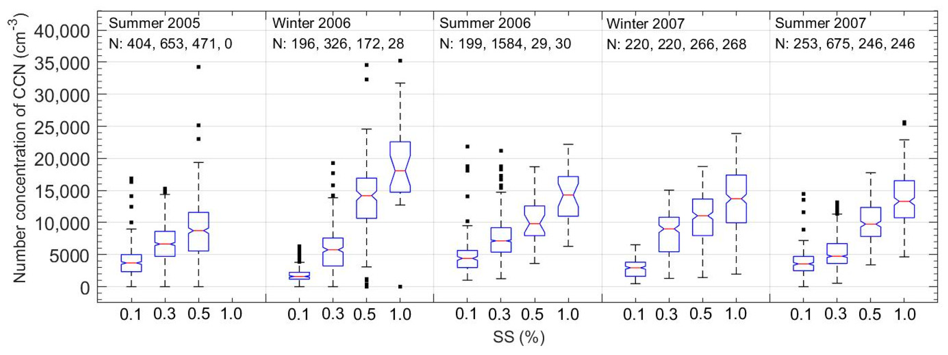
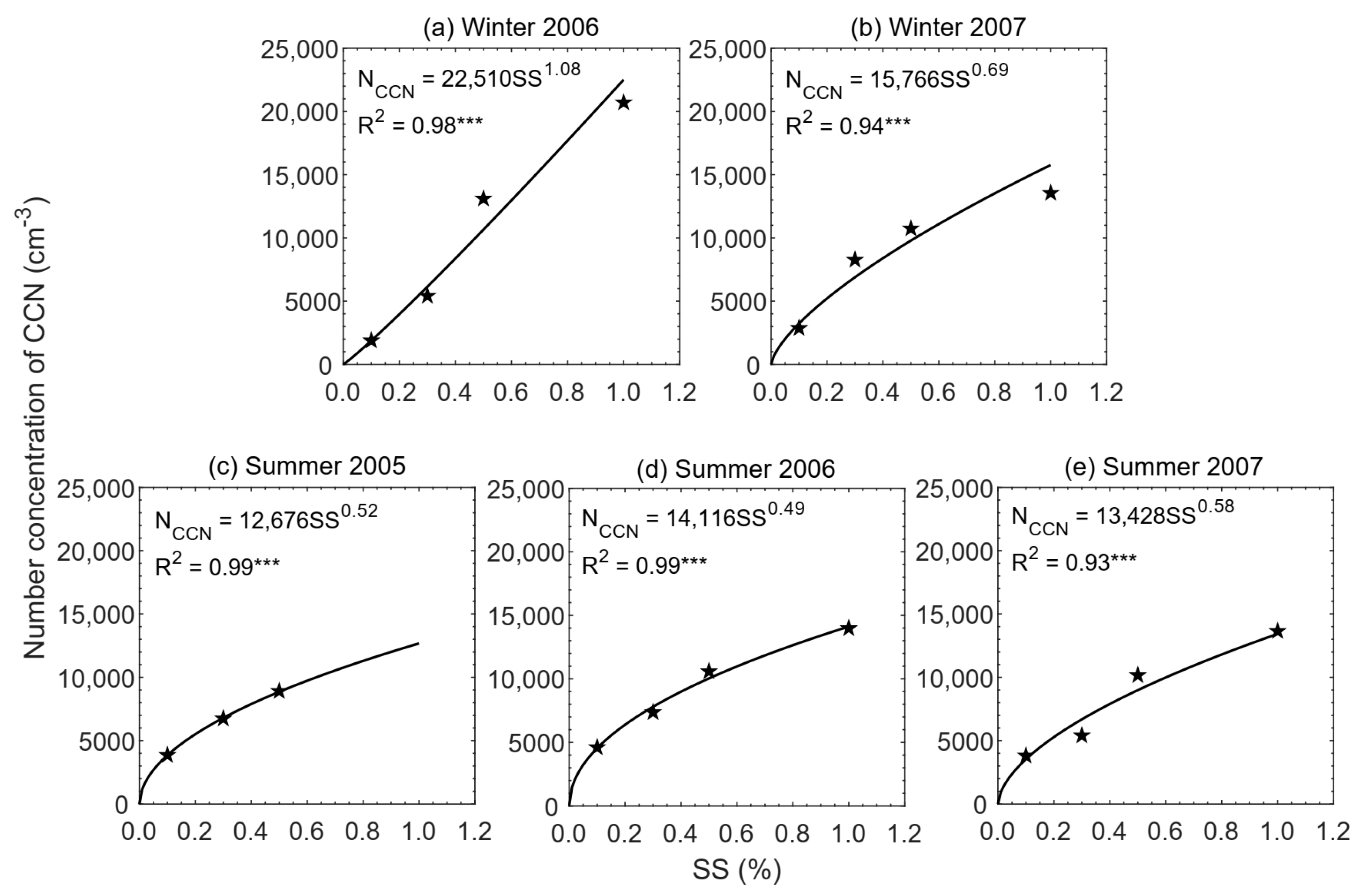
3.4. N_CCN–SS Relationship

An overview of hourly-averaged CCN number concentration is shown in Figure 6. Overall, ${\mathrm{N}}_{\mathrm{CCN}}$ keeps a high level, up to 14,026 ${\mathrm{cm}}^{-3}$ under $\mathrm{SS}=1\%$ in winter, and ${\mathrm{N}}_{\mathrm{CCN}}$ is a little higher in winter than summer, especially at high SS. ${\mathrm{N}}_{\mathrm{CCN}}$ has an increasing tendency with SS in both seasons in Shijiazhuang.

Many empirical formulas have been proposed to obtain ${\mathrm{N}}_{\mathrm{CCN}}$ from the supersaturation (SS). A power-law equation proposed by Twomey [39] is most commonly used, namely ${\mathrm{N}}_{\mathrm{CCN}}={\mathrm{cSS}}^{\mathrm{k}}$. The parameters of $\mathrm{c}$ and $\mathrm{k}$ contain information concerning the particle number concentration and the chemical characteristics of aerosols. We fitted the Twomey formula and obtained the fitting parameters in different periods of this study, as shown in Figure 7. When fitting, we first took the logarithm of both sides of the Twomey formula, that is, $\ln \left({\mathrm{N}}_{\mathrm{CCN}}\right)=\mathrm{kln}\left(\mathrm{SS}\right)+\ln \left(\mathrm{c}\right)$. Next, we used the QR method [65] to linearly fit the above equation (function $\mathrm{lm}$ in R language) using the observed data points to obtain $\mathrm{k}$ and $\ln \left(\mathrm{c}\right)$. The R-squared values were obtained when conducting linear fitting and high ${\mathrm{R}}^2$ denoted a better performance of the fitted curve in representing the observed ${\mathrm{N}}_{\mathrm{CCN}}$–SS relationship (Figure 7). The values of $\mathrm{k}$ in winter (1.08 and 0.69) are larger than those in summer (0.52, 0.49 and 0.58). Therefore, the fitting curves for winter are steeper than the ones for summer (Figure 7). The fitting parameter $\mathrm{c}$ can be regarded as a proxy to represent the particle number concentration. Obviously, the values are higher in winter (22,510 and 15,766) than those in summer (12,676, 14,116 and 13,428). The parameter $\mathrm{c}$ of Shijiazhuang maintaining a high level ($\mathrm{c}\ge 10,000$) in both winter and summer shows the characteristic of a typical continental CCN ($\mathrm{c} \ge 2200$, $\mathrm{k}<1$) [66]. However, we noticed that the fitting parameters in winter 2006 are significantly higher than the results in other years in North China [18,30]. This may be attributed to the highly frequent and severe pollution events in winter 2006 in Shijiazhuang. Qu et al. [46] analyzed the air pollution condition in Shijiazhuang based on the Air Quality Index ($\mathrm{AQI}$). The results showed that there were 5 days with high-polluted events ($\mathrm{AQI}>300$) and 21 days with middle-polluted events ($200<\mathrm{AQI} \le 300$) from 2005 to 2009, and all of the high-polluted events and almost half of middle-polluted events occurred in winter and spring of 2006. Therefore, we think the observations in winter 2007 are more representative of the general air pollution condition in the winter of Shijiazhuang, and the fitting parameters in winter 2006 are more representative of a state of extremely heavy pollution. At the same time, the above results also remind us that it is necessary to consider using larger $\mathrm{c}$ and $\mathrm{k}$ values while using ${\mathrm{N}}_{\mathrm{CCN}}={\mathrm{cSS}}^{\mathrm{k}}$ in heavily polluted areas.

The comparison of parameters $\mathrm{c}$ and $\mathrm{k}$ derived from this study with parameters from different regions (continental or transitional between marine and continental) is shown in

Table 3. Comparison of parameters $\mathrm{c}$ and $\mathrm{k}$ from multiple studies. The type of CCN is determined according to Hobbs et al. [66].

Reference	Time	$\mathbf{c}$	$\mathbf{k}$	Type	Location
Twomey [39]	Spring, 1958	2000	0.40	Transitional	Australia
Hudson [40]	Autumn, 1976	2500	0.70	Continental	San Diego, CA, USA
Martins et al. [41]	Autumn, 2002	2220	1.28	/	Amazonia, Brazil
Wang et al. [18]	Autumn, 2012	4230~17,752	0.49~0.69	Continental	Tianjin, China
Qi and Yao [30]	Winter, 2017	4982~11,689	0.51~0.72	Continental	Qingdao, China
Miao et al. [67]	Summer, 2014	1932	0.53	Transitional	Huangshan, China
This work	Summer, 2005~2007	12,676~14,116	0.49~0.58	Continental	Shijiazhuang, China
	Winter, 2006~2007	15,766~22,510	0.69~1.08

. We found that the value of $\mathrm{c}$ in Shijiazhuang is about one order of magnitude higher than others, which may be related to the high pollution level in Shijiazhuang. Although there is an obvious difference between $\mathrm{c}$ parameters in Shijiazhuang and other studies in China, the values of $\mathrm{k}$ are similar, as shown in Table 3. Qi and Yao [30] studied the CCN characteristics at Qingdao, China in winter and found that the $\mathrm{k}$ values were 0.51~0.72 at different weather conditions. Wang et al. [18] showed that the values of $\mathrm{k}$ were 0.49~0.69 for different wind conditions in autumn of Tianjin, China. Based on the above results, we summarize the recommended values of parameters c and k to construct the fitting formula (${\mathrm{N}}_{\mathrm{CCN}}={\mathrm{cSS}}^{\mathrm{k}}$) when predicting ${\mathrm{N}}_{\mathrm{CCN}}$ in East and North China for a large-scale study. The parameter $\mathrm{c}$ can be obtained from the average value of ${\mathrm{N}}_{\mathrm{CCN}}$ at $\mathrm{SS}=1.0\%$ if the observation data are available. Otherwise, c within the range of 2000 to 15,000 is regarded as a general case, but c > 15,000 should be regarded as the extremely heavy pollution case. The recommended value of parameter k is 0.5–0.7 (0.5 for summer and 0.7 for winter) in East and North China. During the extremely polluted situation, $\mathrm{k}$ needs to be further increased, and it can be selected between 0.7 and 1.0.

4. Conclusions and Discussion

Studying CCN in the atmosphere is of great significance for understanding aerosol–cloud interactions. This study used multi-year data observed in Shijiazhuang from 2005 to 2007 and the reanalysis data (MERRA-2 and ERA5) to investigate the characteristics of CCN, sort the factors affecting the diurnal variation of ${\mathrm{N}}_{\mathrm{CCN}}$ according to their importance, and build the relationship between ${\mathrm{N}}_{\mathrm{CCN}}$ and $\mathrm{SS}$ in the heavily polluted region. Our comprehensive analysis based on CCN long-term observations combined with climate-scale reanalysis data can provide a reference for climatological CCN research analysis or model simulation.

The diurnal variations of ${\mathrm{N}}_{\mathrm{CCN}}$ in different periods show a bimodal distribution, and the peak in the morning is more prominent for summer, but the evening peak is obvious for winter. By analyzing the observation data measured in winter 2007, we found the dominant factor affecting this pattern is the pollutant ${\mathrm{SO}}_2$ in the morning but the pollutant ${\mathrm{NO}}_2$ in the evening, and ${\mathrm{PM}}_{10}$ always maintains a high positive correlation with ${\mathrm{N}}_{\mathrm{CCN}}$ all day. Additionally, we ranked the importance of factors affecting ${\mathrm{N}}_{\mathrm{CCN}}$ diurnal variation by using observation and reanalysis data according to the absolute values of the Pearson correlation coefficient. The variation of pollutants (${\mathrm{C}}_{\mathrm{SO}2}$ and ${\mathrm{C}}_{\mathrm{BC}}$) has the greatest impact on ${\mathrm{N}}_{\mathrm{CCN}}$ in summer, but the variation of atmospheric stability ($\mathrm{BLH}$ and $\mathrm{BLD}$) in winter. To study the relationship between ${\mathrm{N}}_{\mathrm{CCN}}$ and $\mathrm{SS},$ we fitted the Twomey formula (${\mathrm{N}}_{\mathrm{CCN}}={\mathrm{cSS}}^{\mathrm{k}}$) and found the CCN has the typical continental characteristic in Shijiazhuang. According to this study and some previous research, we recommended a reasonable value range (0.5~0.7) of the parameter $\mathrm{k}$ for applying in East and North China. In detail, it is more reasonable for $\mathrm{k}$ to be 0.5 in summer and 0.7 in winter. When extreme pollution ($\mathrm{c}>15,000$) occurs, the value of $\mathrm{k}$ can be further increased, recommending a value between 0.7 and 1.0.

Several points are worthy of mentioning for future studies. Although reanalysis data have great convenience in acquisition and application, these data still have great limitations in the characterization of small-scale regional pollution and meteorological conditions. Therefore, observations of pollutants and meteorological variables on a local scale should be carried out together with ${\mathrm{N}}_{\mathrm{CCN}}$ observations in the future, so as to further improve the understanding of the complex relationship between CCN and pollutants and meteorological conditions. In addition, the ${\mathrm{N}}_{\mathrm{CCN}}$ data used in this study are representative for 2005–2007 only. In recent years, China has achieved remarkable success in pollution control [68], and its impacts on CCN and aerosol–cloud interaction are of interest to study in the future.

References

1. Twomey, S. Pollution and the planetary albedo. Atmos. Environ. 1974, 8, 1251–1256. [Google Scholar] [CrossRef]
2. Twomey, S. The Influence of Pollution on the Shortwave Albedo of Clouds. J. Atmos. Sci. 1977, 34, 1149–1152. [Google Scholar] [CrossRef] [Green Version]
3. Peng, Y.; Lohmann, U.; Leaitch, R.; Banic, C.; Couture, M. The cloud albedo-cloud droplet effective radius relationship for clean and polluted clouds from RACE and FIRE.ACE. J. Geophys. Res. Atmos. 2002, 107, AAC1-1–AAC1-6. [Google Scholar] [CrossRef]
4. Lohmann, U.; Feichter, J. Global indirect aerosol effects: A review. Atmos. Chem. Phys. 2005, 5, 715–737. [Google Scholar] [CrossRef] [Green Version]
5. Albrecht, B.A. Aerosols, Cloud Microphysics, and Fractional Cloudiness. Science 1989, 245, 1227–1230. [Google Scholar] [CrossRef]
6. Forster, P.; Storelvmo, T.; Armour, K.; Collins, W.; Dufresne, J.L.; Frame, D.; Lunt, D.J.; Mauritsen, T.; Palmer, M.D.; Watanabe, M. Climate Change 2021: The Physical Science Basis. Contribution of Working Group I to the Sixth Assessment Report of the Intergovernmental Panel on Climate Change. In Climate Change 2021: The Physical Science Basis. Contribution of Working Group I to the Sixth Assessment Report of the Intergovernmental Panel on Climate Change; Cambridge University Press: Cambridge, UK, 2021. [Google Scholar]
7. Wang, M.; Peng, Y.; Liu, Y. Contrasting Aerosol Effects on Long-Wave Cloud Forcing in South East Asia and Amazon Simulated With Community Atmosphere Model Version 5.3. J. Geophys. Res. Atmos. 2020, 125, e2020JD032380. [Google Scholar] [CrossRef]
8. Xu, L.; Peng, Y.; Ram, K.; Zhang, Y.; Bao, M.; Wei, J. Investigation of the Uncertainties of Simulated Optical Properties of Brown Carbon at Two Asian Sites Using a Modified Bulk Aerosol Optical Scheme of the Community Atmospheric Model Version 5.3. J. Geophys. Res. Atmos. 2021, 126, e2020JD033942. [Google Scholar] [CrossRef]
9. Lee, T.-F.D.; Jiusto, J.E. Diurnal variations in cloud condensation nuclei. J. Geophys. Res. 1974, 79, 5651–5656. [Google Scholar] [CrossRef]
10. Sihto, S.-L.; Mikkilä, J.; Vanhanen, J.; Ehn, M.; Liao, L.; Lehtipalo, K.; Aalto, P.P.; Duplissy, J.; Petäjä, T.; Kerminen, V.-M.; et al. Seasonal variation of CCN concentrations and aerosol activation properties in boreal forest. Atmos. Chem. Phys. 2011, 11, 13269–13285. [Google Scholar] [CrossRef] [Green Version]
11. Leng, C.; Cheng, T.; Chen, J.; Zhang, R.; Tao, J.; Huang, G.; Zha, S.; Zhang, M.; Fang, W.; Li, X.; et al. Measurements of surface cloud condensation nuclei and aerosol activity in downtown Shanghai. Atmos. Environ. 2013, 69, 354–361. [Google Scholar] [CrossRef]
12. Dong, X.; Xi, B.; Wu, P. Investigation of the Diurnal Variation of Marine Boundary Layer Cloud Microphysical Properties at the Azores. J. Clim. 2014, 27, 8827–8835. [Google Scholar] [CrossRef]
13. Kim, J.H.; Yum, S.S.; Shim, S.; Kim, W.J.; Park, M.; Kim, J.-H.; Kim, M.-H.; Yoon, S.-C. On the submicron aerosol distributions and CCN number concentrations in and around the Korean Peninsula. Atmos. Chem. Phys. 2014, 14, 8763–8779. [Google Scholar] [CrossRef] [Green Version]
14. Duan, J.; Chen, Y.; Guo, X. Characteristics of aerosol activation efficiency and aerosol and CCN vertical distributions in North China. Acta Meteorol. Sin. 2012, 26, 579–596. [Google Scholar] [CrossRef]
15. Duan, J.; Lou, X.; Chen, Y.; Gao, Y.; Li, X.; Zhou, R.; Mao, H.; Lu, G.; Wang, H.; Lin, J. Aircraft measurements of aerosol vertical distributions and its activation efficiency over the Pearl River Delta. J. Appl. Meteor Sci. 2019, 30, 677–689. [Google Scholar] [CrossRef]
16. Bhattu, D.; Tripathi, S.N. CCN closure study: Effects of aerosol chemical composition and mixing state. J. Geophys. Res. Atmos. 2015, 120, 766–783. [Google Scholar] [CrossRef]
17. Feng, Q.; Li, Y.; Li, P.; Shen, D.; Jin, L.; Yang, J.; Sun, H. Ground observation of microphysical properties in Shanxi Province. Clim. Environ. Res. 2012, 17, 727–739. [Google Scholar] [CrossRef]
18. Wang, T.; An, L.; Sun, J.; Shen, X.; Zhang, X.; Yan, P.; Deng, Z.; Liang, W.; Zhang, Y.; Chen, L. Variation Characteristics of Cloud Condensation Nuclei at Wuqing. Meteorol. Sci. Technol. 2012, 40, 466–473. [Google Scholar] [CrossRef]
19. Li, Q.; Yin, Y.; Gu, X.; Yuan, L.; Kong, S.; Jiang, Q.; Chen, K.; Li, L. An observational study of aerosol hygroscopic growth factor and cloud condensation nuclei in Nanjing. China Environ. Sci. 2015, 35, 337–346. [Google Scholar]
20. Logan, T.; Dong, X.; Xi, B. Aerosol properties and their impacts on surface CCN at the ARM Southern Great Plains site during the 2011 Midlatitude Continental Convective Clouds Experiment. Adv. Atmos. Sci. 2018, 35, 224–233. [Google Scholar] [CrossRef]
21. Li, Y.; Zhang, F.; Li, Z.; Sun, L.; Wang, Z.; Li, P.; Sun, Y.; Ren, J.; Wang, Y.; Cribb, M.; et al. Influences of aerosol physiochemical properties and new particle formation on CCN activity from observation at a suburban site of China. Atmos. Res. 2017, 188, 80–89. [Google Scholar] [CrossRef]
22. Chen, J.; Li, Z.; Lv, M.; Wang, Y.; Wang, W.; Zhang, Y.; Wang, H.; Yan, X.; Sun, Y.; Cribb, M. Aerosol hygroscopic growth, contributing factors, and impact on haze events in a severely polluted region in northern China. Atmos. Chem. Phys. 2019, 19, 1327–1342. [Google Scholar] [CrossRef] [Green Version]
23. Zhang, F.; Li, Z.; Li, Y.; Sun, Y.; Wang, Z.; Li, P.; Sun, L.; Wang, P.; Cribb, M.; Zhao, C.; et al. Impacts of organic aerosols and its oxidation level on CCN activity from measurement at a suburban site in China. Atmos. Chem. Phys. 2016, 16, 5413–5425. [Google Scholar] [CrossRef] [Green Version]
24. Shi, L.; Duan, Y. Observations of Cloud Condensation Nuclei in North China. Acta Meteorol. Sin. 2007, 65, 97–106. [Google Scholar]
25. Yue, Y.; Niu, S.; Sang, J.; Lv, J. Observational study on the distribution of cloud condensation nuclei and its causes in drought region. China Environ. Sci. 2010, 30, 593–598. [Google Scholar]
26. Liu, J.; Zheng, Y.; Li, Z.; Cribb, M. Analysis of cloud condensation nuclei properties at a polluted site in southeastern China during the AMF-China Campaign. J. Geophys. Res. 2011, 116, D00K35. [Google Scholar] [CrossRef] [Green Version]
27. Feng, Q.; Li, P.; Fan, M.; Hou, T. Observational analysis of cloud condensation nuclei in some regions of North China. Trans. Atmos. Sci. 2012, 35, 533–540. [Google Scholar] [CrossRef]
28. Hsiao, T.-C.; Ye, W.-C.; Wang, S.-H.; Tsay, S.-C.; Chen, W.-N.; Lin, N.-H.; Lee, C.-T.; Hung, H.-M.; Chuang, M.-T.; Chantara, S. Investigation of the CCN Activity, BC and UVBC Mass Concentrations of Biomass Burning Aerosols during the 2013 BASELInE Campaign. Aerosol Air Qual. Res. 2016, 16, 2742–2756. [Google Scholar] [CrossRef] [Green Version]
29. Zhao, Y.; Niu, S.; Lv, J.; Xu, J.; Sang, J. Observational Analyses on Cloud Condensation Nuclei in Northwestern China in Summer of 2007. Plateau Meteorol. 2010, 29, 1043–1049. [Google Scholar]
30. Qi, J.; Yao, X. Observation Analysis of Cloud Condensation Nuclei over Qingdao in Winter. Period. Ocean Univ. 2019, 48, 10–19. [Google Scholar]
31. Che, H.C.; Zhang, X.Y.; Wang, Y.Q.; Zhang, L.; Shen, X.J.; Zhang, Y.M.; Ma, Q.L.; Sun, J.Y.; Zhang, Y.W.; Wang, T.T. Characterization and parameterization of aerosol cloud condensation nuclei activation under different pollution conditions. Sci. Rep. 2016, 6, 24497. [Google Scholar] [CrossRef]
32. Jurányi, Z.; Gysel, M.; Weingartner, E.; Bukowiecki, N.; Kammermann, L.; Baltensperger, U. A 17 month climatology of the cloud condensation nuclei number concentration at the high alpine site Jungfraujoch. J. Geophys. Res. Atmos. 2011, 116, D10204. [Google Scholar] [CrossRef]
33. Pöhlker, M.L.; Pöhlker, C.; Ditas, F.; Klimach, T.; De Angelis, I.H.; Araújo, A.; Brito, J.; Carbone, S.; Cheng, Y.; Chi, X.; et al. Long-term observations of cloud condensation nuclei in the Amazon rain forest—Part 1: Aerosol size distribution, hygroscopicity, and new model parametrizations for CCN prediction. Atmos. Chem. Phys. 2016, 16, 15709–15740. [Google Scholar] [CrossRef] [Green Version]
34. Schmale, J.; Henning, S.; Decesari, S.; Henzing, B.; Keskinen, H.; Sellegri, K.; Ovadnevaite, J.; Pöhlker, M.; Brito, J.; Bougiatioti, A.; et al. Long-term cloud condensation nuclei number concentration, particle number size distribution and chemical composition measurements at regionally representative observatories. Atmos. Chem. Phys. 2018, 18, 2853–2881. [Google Scholar] [CrossRef] [Green Version]
35. Frank, C.W.; Wahl, S.; Keller, J.D.; Pospichal, B.; Hense, A.; Crewell, S. Bias correction of a novel European reanalysis data set for solar energy applications. Sol. Energy 2018, 164, 12–24. [Google Scholar] [CrossRef]
36. Jiang, H.; Yang, Y.; Bai, Y.; Wang, H. Evaluation of the Total, Direct, and Diffuse Solar Radiations from the ERA5 Reanalysis Data in China. IEEE Geosci. Remote Sens. Lett. 2020, 17, 47–51. [Google Scholar] [CrossRef]
37. Mahto, S.S.; Mishra, V. Does ERA-5 Outperform Other Reanalysis Products for Hydrologic Applications in India? J. Geophys. Res. Atmos. 2019, 124, 9423–9441. [Google Scholar] [CrossRef]
38. Chen, S.; Gan, T.Y.; Tan, X.; Shao, D.; Zhu, J. Assessment of CFSR, ERA-Interim, JRA-55, MERRA-2, NCEP-2 reanalysis data for drought analysis over China. Clim. Dyn. 2019, 53, 737–757. [Google Scholar] [CrossRef]
39. Twomey, S. The nuclei of natural cloud formation part II: The supersaturation in natural clouds and the variation of cloud droplet concentration. Geofis. Pura Appl. 1959, 43, 243–249. [Google Scholar] [CrossRef]
40. Hudson, J.G. Relationship between fog condensation nuclei and fog microstructure. J. Atmos. Sci. 1980, 37, 1854–1867. [Google Scholar] [CrossRef] [Green Version]
41. Martins, J.A.; Gonçalves, F.L.T.; Morales, C.A.; Fisch, G.F.; Pinheiro, F.G.M.; Leal, B.V., Jr.; Oliveira, C.J.; Silva, E.M.; Oliveira, J.C.P.; Costa, A.A.; et al. Cloud condensation nuclei from biomass burning during the Amazonian dry-to-wet transition season. Meteorol. Atmos. Phys. 2009, 104, 83–93. [Google Scholar] [CrossRef]
42. Huang, J.; Pan, X.; Guo, X.; Li, G. Health impact of China’s Air Pollution Prevention and Control Action Plan: An analysis of national air quality monitoring and mortality data. Lancet Planet. Health 2018, 2, e313–e323. [Google Scholar] [CrossRef] [Green Version]
43. Cai, S.; Wang, Y.; Zhao, B.; Wang, S.; Chang, X.; Hao, J. The impact of the “Air Pollution Prevention and Control Action Plan” on PM2.5 concentrations in Jing-Jin-Ji region during 2012–2020. Sci. Total Environ. 2017, 580, 197–209. [Google Scholar] [CrossRef] [PubMed]
44. Sogacheva, L.; De Leeuw, G.; Rodriguez, E.; Kolmonen, P.; Georgoulias, A.K.; Alexandri, G.; Kourtidis, K.; Proestakis, E.; Marinou, E.; Amiridis, V.; et al. Spatial and seasonal variations of aerosols over China from two decades of multi-satellite observations -Part 1: ATSR (1995–2011) and MODiS C6.1 (2000–2017). Atmos. Chem. Phys. 2018, 18, 11389–11407. [Google Scholar] [CrossRef] [Green Version]
45. Wei, J.; Peng, Y.; Mahmood, R.; Sun, L.; Guo, J. Intercomparison in spatial distributions and temporal trends derived from multi-source satellite aerosol products. Atmos. Chem. Phys. 2019, 19, 7183–7207. [Google Scholar] [CrossRef] [Green Version]
46. Qu, X.; Fu, G.; Jia, J.; Yang, G. Distribution characteristics of air quality and its relationship with meteorological factors from 2005 to 2009 in Shijiazhuang, Hebei province. J. Meteorol. Environ. 2011, 27, 29–32. [Google Scholar]
47. Xu, W.Y.; Zhao, C.S.; Ran, L.; Deng, Z.Z.; Liu, P.F.; Ma, N.; Lin, W.L.; Xu, X.B.; Yan, P.; He, X.; et al. Characteristics of pollutants and their correlation to meteorological conditions at a suburban site in the North China Plain. Atmos. Chem. Phys. 2011, 11, 4353–4369. [Google Scholar] [CrossRef] [Green Version]
48. Roberts, G.C.; Nenes, A. A continuous-flow streamwise thermal-gradient CCN chamber for atmospheric measurements. Aerosol Sci. Technol. 2005, 39, 206–221. [Google Scholar] [CrossRef]
49. Ward, D.S.; Cotton, W.R. Cold and transition season cloud condensation nuclei measurements in western Colorado. Atmos. Chem. Phys. 2011, 11, 4303–4317. [Google Scholar] [CrossRef] [Green Version]
50. Gelaro, R.; McCarty, W.; Suárez, M.J.; Todling, R.; Molod, A.; Takacs, L.; Randles, C.A.; Darmenov, A.; Bosilovich, M.G.; Reichle, R.; et al. The Modern-Era Retrospective Analysis for Research and Applications, Version 2 (MERRA-2). J. Clim. 2017, 30, 5419–5454. [Google Scholar] [CrossRef]
51. Xing, Z.; Li, S.; Xiong, Y.; Du, K. Estimation of cross-boundary aerosol flux over the Edmonton-Calgary Corridor in Canada based on CALIPSO and MERRA-2 data during 2011–2017. Atmos. Environ. 2021, 246, 118084. [Google Scholar] [CrossRef]
52. Sun, E.; Che, H.; Xu, X.; Wang, Z.; Lu, C.; Gui, K.; Zhao, H.; Zheng, Y.; Wang, Y.; Wang, H.; et al. Variation in MERRA-2 aerosol optical depth over the Yangtze River Delta from 1980 to 2016. Theor. Appl. Climatol. 2019, 136, 363–375. [Google Scholar] [CrossRef]
53. McCoy, D.T.; Bender, F.A.-M.; Mohrmann, J.K.C.; Hartmann, D.L.; Wood, R.; Grosvenor, D.P. The global aerosol-cloud first indirect effect estimated using MODIS, MERRA, and AeroCom. J. Geophys. Res. Atmos. 2017, 122, 1779–1796. [Google Scholar] [CrossRef]
54. Zhao, Q.; Zhao, W.; Bi, J.; Ma, Z. Climatology and calibration of MERRA-2 PM2.5 components over China. Atmos. Pollut. Res. 2021, 12, 357–366. [Google Scholar] [CrossRef]
55. Ma, X.; Yan, P.; Zhao, T.; Jia, X.; Jiao, J.; Ma, Q.; Wu, D.; Shu, Z.; Sun, X.; Habtemicheal, B.A. Article evaluations of surface pm10 concentration and chemical compositions in merra-2 aerosol reanalysis over central and eastern China. Remote Sens. 2021, 13, 1317. [Google Scholar] [CrossRef]
56. Qin, W.; Zhang, Y.; Chen, J.; Yu, Q.; Cheng, S.; Li, W.; Liu, X.; Tian, H. Variation, sources and historical trend of black carbon in Beijing, China based on ground observation and MERRA-2 reanalysis data. Environ. Pollut. 2019, 245, 853–863. [Google Scholar] [CrossRef] [PubMed]
57. Wang, Q.; Li, W.; Xiao, C.; Ai, W. Evaluation of high-resolution crop model meteorological forcing datasets at regional scale: Air temperature and precipitation over major land areas of China. Atmosphere 2020, 11, 1011. [Google Scholar] [CrossRef]
58. Jiang, Y.; Han, S.; Shi, C.; Gao, T.; Zhen, H.; Liu, X. Evaluation of HRCLDAS and ERA5 Datasets for Near-Surface Wind over Hainan Island and South China Sea. Atmosphere 2021, 12, 766. [Google Scholar] [CrossRef]
59. Benesty, J.; Chen, J.; Huang, Y.; Speech, I.C.-N. Pearson Correlation Coefficient. In Noise Reduction in Speech Processing; Springer: Berlin/Heidelberg, Germany, 2009. [Google Scholar]
60. Zhang, F.; Wang, Y.; Peng, J.; Ren, J.; Collins, D.; Zhang, R.; Sun, Y.; Yang, X.; Li, Z. Uncertainty in Predicting CCN Activity of Aged and Primary Aerosols. J. Geophys. Res. Atmos. 2017, 122, 11723–11736. [Google Scholar] [CrossRef]
61. Wang, Y.; Zhang, F.; Li, Z.; Tan, H.; Xu, H.; Ren, J.; Zhao, J.; Du, W.; Sun, Y. Enhanced hydrophobicity and volatility of submicron aerosols under severe emission control conditions in Beijing. Atmos. Chem. Phys. 2017, 17, 5239–5251. [Google Scholar] [CrossRef] [Green Version]
62. Duan, X.; Jiang, Y.; Wang, B.; Zhao, X.; Shen, G.; Cao, S.; Huang, N.; Qian, Y.; Chen, Y.; Wang, L. Household fuel use for cooking and heating in China: Results from the first Chinese Environmental Exposure-Related Human Activity Patterns Survey (CEERHAPS). Appl. Energy 2014, 136, 692–703. [Google Scholar] [CrossRef]
63. Chai, L.; Ma, C.; Ni, J.Q. Performance evaluation of ground source heat pump system for greenhouse heating in northern China. Biosyst. Eng. 2012, 111, 107–117. [Google Scholar] [CrossRef]
64. Liu, H.; He, K.; Barth, M. Traffic and emission simulation in China based on statistical methodology. Atmos. Environ. 2011, 45, 1154–1161. [Google Scholar] [CrossRef]
65. Kublanovskaya, V.N. On some algorithms for the solution of the complete eigenvalue problem. USSR Comput. Math. Math. Phys. 1962, 1, 637–657. [Google Scholar] [CrossRef]
66. Hobbs, P.V.; Bowdle, D.A.; Radke, L.F. Particles in the lower troposphere over the high plains of the United States. Part II: Cloud condensation nuclei. J. Clim. Appl. Meteorol. 1985, 24, 1358–1369. [Google Scholar] [CrossRef] [Green Version]
67. Miao, Q.; Zhang, Z.; Li, Y.; Qin, X.; Xu, B.; Yuan, Y.; Gao, Z. Measurement of cloud condensation nuclei (CCN) and CCN closure at Mt. Huang based on hygroscopic growth factors and aerosol number-size distribution. Atmos. Environ. 2015, 113, 127–134. [Google Scholar] [CrossRef]
68. Dou, X.; Liao, C.; Wang, H.; Huang, Y.; Tu, Y.; Huang, X.; Peng, Y.; Zhu, B.; Tan, J.; Deng, Z.; et al. Estimates of daily ground-level NO2 concentrations in China based on Random Forest model integrated K-means. Adv. Appl. Energy 2021, 2, 100017. [Google Scholar] [CrossRef]
Figure 1. The location of the study area and the observed periods in this study. (a) The location of the Beijing-Tianjin-Hebei region (red box) in the world map; (b) the location of Shijiazhuang in the Beijing-Tianjin-Hebei region and its topographic map. (c) Sampling stations (colored points, OBS_S: Hebei Meteorological Service Station; OBS_E: Environmental Monitoring Center; OBS_M: Meteorological Observation Station), as well as the extraction area (blue box) for obtaining the reanalysis data; (d) the observed periods include summer 2005, winter 2006, summer 2006, winter 2007, and summer 2007 (detailed time is listed in Table 1).
Atmosphere 13 00468 g001
Figure 2. The diurnal variation of N CCN in different periods under   SS = 0.3 % . (a) The absolute variations of N CCN in winter and summer; (b,c) are normalized results for summer ( N CCN ( summer ) ) and winter ( N CCN ( winter ) ), respectively. Data can be found in the supplementary materials.
Atmosphere 13 00468 g002
Figure 3. The diurnal variations of normalized pollutants and N CCN values in winter 2007, including (a)   M NO 2 , (b)   M PM 10 , and (c)   M SO 2 , respectively. The Pearson correlation coefficients for the whole day ( r ), a.m. ( r a . m . ), and p.m. ( r p . m . ) are shown in the top left of each graph. Superscripts *** and ** indicate that the fitting parameters pass the consistency test under the significance levels of 99% and 95%, respectively.
Atmosphere 13 00468 g003
Figure 4. The hourly-averaged diurnal variations (normalized) of (a,d) pollutants ( C SO 2 ,   C O 3 , C BC and M Dust ), (b,e) meteorological variables ( T O ,   WS 10 O , WS and RH ), (c,f) atmospheric stability variables ( BLH ,   BLD ,   CAPE and CIN ), and N CCN in summer (top panels) and winter (bottom panels) during 2005 and 2007. The r value represents the strength of correlation between the individual variable and N CCN is shown in the bracket. The superscripts of ***, **, and * present the correlations passing the consistency test with the significance levels of 99%, 95% and 90%, respectively.
Atmosphere 13 00468 g004
Figure 5. A chord diagram to display the correlation relationships (represented with the absolute value of r ) between pollutants (black arcs of the circumference; C SO 2 ,   C O 3 , C BC and M Dust ), meteorological variables (dark grey arcs; T O ,   WS 10 O , WS , and RH ) and atmospheric stability variables (grey arcs; BLH ,   BLD and   CAPE ) and N CCN in summer (red arc) and winter (blue arc). The absolute values of r (numbers shown along the upper half circumference) denote the correlations between the corresponding variables and N CCN connected by the red/blue belt. The wider belt indicates the stronger correlation between the individual variable and N CCN .
Atmosphere 13 00468 g005
Figure 6. An overview of hourly–averaged   N CCN . All the data are divided into five groups that present different observation periods. Each group contains four SS levels, namely 0.1%, 0.3%, 0.5% and 1.0%. “N” means the number of samples in different SS. On each box, the central mark (red line) indicates the median, and the bottom and top edges (blue line) of the box indicate the 25th and 75th percentiles, respectively. The outliers are plotted individually using the point symbol.
Atmosphere 13 00468 g006
Figure 7. The relationship between   N CCN and SS in (a) winter 2006, (b) winter 2007, (c) summer 2005, (d) summer 2006 and (e) summer 2007. The fitting formulas and the corresponding R–squared ( R 2 ) values are marked on the upper left of each graph. Stars and the solid curve in each panel represent the observed data points and the fitted curve of N CCN –SS relationship, with the SS ranging from 0 to 1%. The superscript, ***, indicates that the fitting parameters pass the consistency test under the significance levels of 99%.
Atmosphere 13 00468 g007