Identification of Concurrent Clear-Air and Precipitation Doppler Profiles for VHF Radar and an Incorporating Study of Strongly Convective Precipitation with Dual-Polarized Microwave Radiometer

Abstract

Two approaches were designed to identify the echoes of clear air and precipitation when both coexist in the very-high-frequency (VHF) radar spectra: contour-based and peak-finding methods. The contour-based approach was used to model a 2D Doppler spectra to determine the locations of multiple spectral humps, and the peak-finding approach was used to find the spectral peaks on request. Grouping, sifting, and Gaussian fitting were performed further for such obtained contour centres and spectral peaks to yield Doppler velocities and spectral widths. In general, the two approaches resulted in corresponding outcomes and can be complementary to find the spectral peaks as fully as possible. The Doppler velocities retrieved from the two approaches were cooperatively used to develop an effective process of Doppler profiling for treating a great amount of radar data, which was validated with the radar data collected during a rainy and strongly convective atmosphere. As an application of Doppler profiling results, the hydrometeor parameters measured by a dual-polarized microwave radiometer were investigated jointly with radar observation, showing that a strong updraft air could bring the liquid water to a height above the melting layer and then the Bergeron effect and coalescence processes on formation of ice crystals and graupel particles occur accordingly.

1. Introduction

Atmospheric radars operated at very-high-frequency (VHF) and ultra-high-frequency (UHF) bands are powerful instruments in remote sensing of the atmosphere from troposphere to ionosphere. In addition to the clear-air turbulence and plasma irregularities, precipitation is also a significant source of the radar echoes, which has been extensively investigated for decades (e.g., [1,2,3,4,5,6]).

Wind velocity is a basic measurement of using VHF/UHF atmospheric radars. Due to radio interference echoes or unwanted signals, such as those from airplanes, birds, radio frequencies, and so on, wind velocity is estimated erroneously. Moreover, the ground clutter that produces a significant peak in the Doppler spectrum around zero velocity can be a problem for some radars. A simple way to mitigate the influence of ground clutter is via the removal of direct current (DC) from the raw data and/or average of both sides of the spectral lines around zero velocity. To remove the contamination of ground clutter more effectively, however, several sophisticated algorithms have been developed, e.g., neural network [7], Genetic algorithm [8] and Fuzzy logic-based methods [9,10]. After suppressing the signals of ground cutters or other interferences, tracing the Doppler profiles of the echoes throughout the height is more applicable. For example, Anandan et al. [11] proposed an adaptive moments estimation technique and Sinha et al. [12] used a multiparameter cost function method to trace the Doppler profile of clear-air motion in low signal-to noise ratio (SNR) condition, in which the wind-shear value is an important criterion in tracing.

The aforementioned algorithms and tracings focused on extracting the Doppler velocity of clear-air motion. In case of strong hydrometeor echoes that are closer to the clear-air echoes in the Doppler spectrum, Gan et al. [13] proposed a two-echo method to exclude the hydrometeor or precipitation echoes so that the spectral parameters (Doppler velocity and spectral width) of clear air could be estimated more accurately. In addition, Kumer et al. [14] recently proposed a so-called symmetric method to identify and separate the turbulence echoes from the multi-peaked VHF radar spectra during precipitation and validated the symmetric method against a two-frequency method [15]. The precipitation echoes, on the other hand, are useful for estimating the drop size distribution (DSD) of falling hydrometers, and DSD is an essential measurement of deducing the rainfall rate, liquid water content, terminal velocity of hydrometer, and so on [16,17]. Therefore, the clear-air echoes should be removed from the observed Doppler spectrum for extraction of precipitation echoes, and several methods have been explored for this purpose. For example, deconvolution operation [1,18], spectral fitting [19,20,21], cluster analysis [22], peak-searching process for the air spectrum [23], and others based on these methods [24,25]. For the microwave radars used exclusively for observations of hydrometers, there were also fine algorithms developed for distinguishing multiple spectral peaks that may represent different species of hydrometeors [26,27]. Recognition of diverse hydrometers, however, is difficult for VHF radars due to the much longer wavelengths in the VHF band than in the microwave band.

Although there have been a few methods applicable to the identification of multiple peaks in the radar spectra, we intend to propose additional approaches with some basic data analysis techniques to this issue for future studies with VHF radar; that is, contour-based and peak-finding processes. The two proposed approaches attempt to find the locations of spectral humps that represent the clear-air and precipitation echoes as fully as possible and then group and sift these spectral locations with some suitable criteria. With applicable locations of spectral humps, Doppler profiling for respective echoes of clear air and precipitation can then be achieved. To validate the usability of the proposed approaches and profiling process, a strongly convective atmosphere detected by the Chung-Li VHF radar was selected for demonstration. This convective atmosphere occurred when typhoon Trami passed the island of Taiwan in August 2013, leading to wide variations in Doppler velocity and spectral width, and thereby yielding an excellent testbed for identifying approaches and the profiling process.

Finally, as an application of Doppler profiling results and an extended study on the convective precipitation observed, the hydrometeor parameters (brightness temperature, liquid water content, and so on) measured by a dual-polarization microwave radiometer and the spectral parameters observed by the VHF radar were inspected jointly to survey the interrelation between hydrometeor particles and clear-air turbulence in such a strongly convective atmosphere. There are a few collaborative studies with VHF/UHF radar and microwave radiometer in the literature that aimed at atmospheric humidity or temperature profiling [28,29,30,31]. In this paper, however, the Bergeron effect and coalescence process above the melting layer are discussed.

This paper is organized as follows. In Section 2, the two approaches developed in this study are described. Section 3 presents some characteristics of the retrieved spectral parameters. Comparisons between the spectral parameters obtained from the two approaches, different FFT numbers, and clear-air and precipitation echoes are given. Section 4 addresses the process to trace the respective Doppler profiles of concurrent clear-air and precipitation echoes. Advantages and limitations of the tracing process will be discussed. Finally, co-observations of precipitation with VHF radar and dual-polarized microwave radiometer are shown in Section 5, where the spectral parameters, estimated from the proposed approaches, and the hydrometeor parameters, provided by the radiometer, are jointly discussed. Conclusions are drawn in Section 6.

2. Methodology and Data Analysis

A flowchart that briefly describes the procedures of estimating Doppler spectral parameters is shown in Figure 1, which includes the pre-processing of radar data, two approaches of peak identification (contour-based and peak-finding), estimates of Doppler velocity and spectral width, and the Doppler profiling process (detailed in Section 4).

2.1. Pre-processing

First, Doppler spectra of the radar echoes were produced by using fast Fourier transform (FFT), in which the DC component had been removed in advance. For some purpose of study shown later, the FFTs with 32, 64 and 128 raw data pints were performed, respectively. As known, the FFT spectrum of a finite-length data is the convolution result of the true spectra and the frequency response of a time window framing the finite data, in which the frequency response of a time window is a sinc function governed by the reciprocal of the time window length. The wider the time window, the narrower the main lobe of the sinc function, and then the less effect on the spectra. A longer data length also yields a higher spectral resolution but might contain more various signals each time of FFT and provide a more fluctuated spectrum. In addition, signal-to-noise ratio (SNR) is another factor fluctuating the spectral shape. Accordingly, it is expected that the resultant spectral parameters could vary more or less with data length. We examined this issue intentionally in Section 3.2.

Incoherent integration times of 4, 2 and 1 were executed, respectively, for the 32-, 64- and 128-point Doppler spectra to render the Doppler spectra with the same time duration, i.e., 16.384 s, which was estimated from a sampling time of 0.128 s given in the VHF radar observation. In addition, the positive Doppler range was extended to about 16 m/s to include a more complete spectral lines of precipitation when the falling velocity of precipitation (downward was positive) exceeded the Nyquist Doppler velocity (~11 m/s). This was carried out by copying the one fourths spectra on the leftmost side to the rightmost side. Such extension of Doppler spectral range is beneficial for locating the spectral peaks of precipitation at large Doppler velocities. The copying, nevertheless, is not always necessary if the sampling time is so short that the Nyquist Doppler velocity is much larger than the Doppler velocity of precipitation.

After extension of the Doppler spectral range, 3-, 7-, and 13-point equal-weight running mean were applied to the Doppler spectra of 32-, 64- and 128-point FFT, respectively. Both running mean and incoherent integration can smooth the spectral curve. However, we should not expect that the smoothed spectral curve ascends and descends monotonically on both sides of a single peak always. Practical spectral curve could be bifurcated on a spectral hump, making the identification of spectral peaks laborious sometimes.

2.2. Identification of Spectral Peaks

To identify the spectral peaks in varied Doppler spectra, the contour-based and peak-finding approaches were designed in this study. There are several parameters and criteria given initially in the identification process, of which the purpose is to develop an identification process that can fit the characteristics of VHF radar echoes. Changes in these parameters and criteria surely produces different outcomes, but we can expect to find a set of parameters and criteria that are suitable for most circumstances and thereby applicable for Doppler profiling.

2.2.1. Contour-Based Approach

For clarity, the processing is stated step by step. Graphical examples are from the 64-point FFT spectrum.

• Modelling of 2-D spectra

The original 1-D Doppler spectrum was first extended purposely to another orthogonal spectral dimension with a Gaussian function for each spectral line to construct a modelled 2-D Doppler spectrum, in which the height of the spectral line and a spectral width were assigned, respectively, to the peak value and the standard deviation of the Gaussian function. Note that the assignment of a spectral width is arbitrary. It is just to model a 2-D Doppler spectrum for the contour method, and in theory different spectral widths given to the extended spectral dimension do not alter the contour centre at the true spectral axis. In this study, one eighth of the FFT number was given to the spectral width of the extended spectral dimension (e.g., 8 for 64-point FFT).

2.

Acquisition of contour lines

The built-in function C = contour(S, N) in the MATLAB software was employed to obtain the contour lines of the modelled 2-D spectrum, where S is the matrix of the 2-D spectrum in linear scale, N is the contour levels, and C is the matrix containing the coordinates of the obtained contour lines. The contour levels were given to be adaptive to the maximum value M₀ of the spectral lines in accordance with a relation given below:

N = 2 + floor[1 0 log10(M_o)]

(1)

where “floor” is the MATLAB function that rounds the value to the nearest integer less than or equal to that value. As a result, the number of contour levels is larger for a higher M₀ so that some minor contour centres can also be identified for later investigation. To avoid the negative value of N, however, only the value of M₀ larger than 1 was processed. Accordingly, the minimum of N was 2. Figure 2 shows one example, where the power spectrum after running mean is shown in panel (a), and the contour lines are present in panel (b). The five plus symbols indicate the contour centres determined in the next step.

3.

Determination of contour centres

With the coordinates of contour lines, C, the contour centres were determined by applying the locating process proposed by Chen et al. [32]. Briefly, the centroid of coordinates of the contour line with the maximum level surrounding the spectral peak are estimated to represent the contour centre, for example, the five pluses shown in Figure 2b. In theory, the contour centre is situated at the dimension of the original 1-D Doppler spectrum because the modelled Doppler spectrum in the orthogonal dimension does not deviate the contour centre from the original Doppler spectral dimension, except a tiny error from computation. Therefore, in the following statement, the location of the contour centre is the coordinate of the contour centre in the original Doppler spectral dimension. Additionally, note that the location of the contour centre does not necessarily coincide exactly with the spectral peak point surrounded by the contour line.

At most, five contour centres that are the most significant were selected through the process mentioned above. Two examples are shown in Figure 3. In Figure 3a, the Doppler spectrum (solid curve, normalized) shows three spectral humps, which has been shown in Figure 2a. The spectral lines around the leftmost peak were aliasing spectra coming from the rightmost part of the spectra, which arose from the finite Nyquist frequency and was ruled out in the contouring process. The central and rightmost peak regions represented the clear-air and precipitation echoes, respectively, which are comparable. Five contour centres were determined, as indicated by the red dots in Figure 3a. Note that the dots and x-shaped symbols in black were from the peak-finding approach, which will be explained later.

As seen in Figure 3a, the identified contour centres were either untypical (number 3) or arose from bifurcation in a spectral hump (1 and 2, 4 and 5). In view of this, the grouping and sifting of these contour centres are necessary. We employed a velocity interval (v_interval) to group the contour centres, in which the value of 1.4 m/s was given for v_interval. All the contour centres within v_interval were adopted to calculate a weighted mean centre, where the respective maximum contour levels of the contour centres were used as the weights in the calculation of mean centre. With the sampling time of 0.128 s, 1.4 m/s corresponded to 2-, 4-, and 8-times that of the spectral resolutions in 32-, 64-, and 128-point FFT spectra, respectively. Two times the spectral resolution is the minimum separation of adjacent spectral peaks. Based on this, the value of 1.4 m/s was used reasonably. Subject to this criterion, the contour centres 1 and 2 fused into a mean centre, and the contour centres 3-5 were retained. After grouping, another criterion of spectral power was used to sift the mean and the remaining contour centres (mean centre thereafter). The mean centre was retained only when the ratio of the spectral power, averaged from several spectral lines centred on the mean centre, to a referenced noise level was higher than a specified threshold value (R_p), say, 0.75 in this study. Giving a higher R_p will reject more minor mean centres. Here, the referenced noise level was estimated from the mean of the lowest one fourths spectral power lines, and the averaged spectral power of each mean centre was calculated from 6, 10, and 14 spectral lines centred on the mean centre, respectively, for the Doppler spectra of 32-, 64-, and 128-point FFT. This number set of spectral lines can include the spectral peaks grouped within 1.4 m/s. After grouping and sifting, four mean centres remained, as denoted by the x-shaped symbols in red.

Figure 3b shows another example where the clear-air echo intensity (the spectral hump around 0 m/s) was much larger than that of precipitation (the spectral hump around 4 m/s). Four contour centres were determined initially (red dots). After grouping and sifting for the four contour centres, only two centres were retained, as indicated by the x-shaped symbols in red.

2.2.2. Peak-Finding Approach

The peak-finding method is commonly employed in several of the aforementioned algorithms for identification of multiple spectral peaks. We have developed our own process for the study. The processing is similar to the third step of the contour-based approach, except that the function “findpeaks” built in MATLAB was used to find the five most significant spectral peaks that were separated by at least a velocity interval (v_interval). v_interval was given as that in the contour-based approach. Two examples have been shown in Figure 3, as indicated by the black dots. As seen clearly in the two examples, not all of the spectral peaks coincided with the contour centres (red dots).

Grouping and sifting of these initially obtained spectral peaks were the same as those made in the contour-based approach. As a result, four peaks survived in Figure 3a, and only three peaks remained in Figure 3b, as indicated by the x-shaped symbols in black. The leftmost spectral peak in Figure 3a was ruled out in the sifting process as it was very close to the starting point and therefore could not provide an estimate of spectral power with 10 spectral lines centred on the spectral peak. The situation was the same for the spectral peak (and contour centre) close to the right boundary. In addition, not all of the spectral peaks surviving here are effective; some of them were ruled out further in the Gaussian fitting, as described in the next section.

2.3. Estimation of Doppler Velocity and Spectral Width

To obtain the spectral parameters (Doppler velocity and spectral width) of various targets in the spectra, Gaussian fitting was performed for each mean centre and spectral peak processed in Section 2.2. The fitting was carried out, respectively, with 5, 7, 9, 11, and 13 spectral lines centred on the mean centre or spectral peak. Such repetitive fitting is based on the truth that the fitting could fail when the selected spectral lines are not complete for the spectral hump. After all, the width of the spectral hump (i.e., spectral width) is unknown in advance. We expect that among the five fittings, at least one is effective. Each fitted Gaussian curve yields a pair of peak location and standard deviation, representing Doppler velocity and spectral width, respectively. As a result, for the four processed mean centres denoted by red x-shaped symbols in Figure 3a, only two of them provided available Gaussian curves, as shown in Figure 4a. The same process of Gaussian fitting was also performed for the spectral peaks denoted by the black x shapes in Figure 3; the fitting results are not shown here to save space.

The fitted Gaussian curves are candidates for the spectral parameters. However, the Gaussian peak location deviating from the processed mean centre (or spectral peak) to some degree was ruled out as a candidate, i.e., the separation, a half of the velocity interval (v_interval = 1.4 m/s), was a distance threshold of accepting or discarding the Gaussian curve. Among the final candidates, we adopted the Gaussian curve with the smallest standard deviation. The reasons for such a selection are: (1) finite data length (resulting in a sinc function in frequency domain), and incoherent integration and running mean of spectrum tend to broad the spectral width; and (2) beam broadening effect on spectral width exists commonly, which is associated with horizontal wind. It is expected that such collected spectral widths can represent the characteristics of turbulence and precipitation to a greater degree. A quantitative study of the broadening effect on spectral width is beyond the scope of this study and was not examined further.

For the two groups of Gaussian curves in Figure 4a, the Gaussian curve from 5-point fitting had the smallest standard deviation for both spectral humps, as indicated by the black dotted-curves. By contrast, among the fitted Gaussian curves in Figure 4b, the 7-point fitting (blue dotted-curve) yielded the smallest width for both spectral humps, which was different from the preceding example. In addition, only three Gaussian fittings with 7, 9, and 11 points were obtained for the minor spectral hump around 4 m/s, and among them the curves resulting from 9- and 11-point fitting were extremely broad and deviated from the mean centre significantly. In view of such variable outcomes of Gaussian fitting, criteria for choice of suitable Gaussian curve are required.

The resultant Doppler velocity and spectral width are displayed in Figure 5, as denoted by the dot and the horizontal bar crossing the dot. Red dots show the outcomes of the contour-based approach, and the black dots are the results obtained from the peak-finding approach. Additional calculations, as present with open circles, were obtained from the moment method using the spectral lines centred on the Gaussian-fitted Doppler velocity in the peak-finding approach. The spectral lines contained in the moment calculation were within two-times that of the Gaussian-fitted standard deviation on both sides of the Gaussian-fitted Doppler velocity. That means that the spectral lines within the 95% area of the Gaussian-fitted curve were used. The purpose of this additional calculation was to compare the results of Gaussian fitting and moment method. As seen, the three pairs of Doppler velocity and spectral width were close to each other for the example shown in Figure 5a. By contrast, for the example shown in Figure 5b, only the contour-based approach yielded the spectral parameter of the minor hump peaked at around 4 m/s. Nevertheless, there were examples that the peak-finding approach provided outcomes, but the contour-based approach did not (not shown). In view of this, the two approaches can be complementary in finding meaningful spectral parameters, which is beneficial for tracking the varied Doppler profiles.

3. Statistical Characteristics of Spectral Parameters

The two examples demonstrated in Figure 5 have shown that the two proposed approaches and the additional moment-method calculation could yield different Doppler velocities and spectral widths sometimes. In view of this, more statistical comparisons between the spectral parameters retrieved from the proposed methods are shown in Section 3.1. Moreover, as mentioned in Section 2.1, different time windows give different frequency resolutions as well as unequal spans of sinc function in frequency domain, and thereby the resultant spectral parameters could vary with data length more or less. Therefore, it is important to discuss on this issue; this is given in Section 3.2. To demonstrate a potential application with the retrieved spectral parameters, comparison between the spectral widths of clear-air and precipitation echoes are provided in Section 3.3.

The above-mentioned investigations were carried out with the Chung-Li VHF radar data collected on 21 August 2013, when the typhoon Trami just passed through the Taiwan area and caused heavy convective precipitation. The radar parameters were set as follows: vertically transmitted radar beam with multiple carrier-frequency mode (i.e., the carrier frequencies of 51.5, 51.75, 52, 52.25, and 52.5 MHz were transmitted alternately), inter-pulse period 200 μs, number of coherent integrations 128, pulse width 1 μs, sampling interval 1 μs (corresponding to a range step of 150 m), lowest sampling height 1.5 km, number of range gates 80, and without pulse coding. As a result, the sampling time of radar returns for each carrier frequency was 0.128 s (=200 μs × 128 integration times × 5 frequencies). For the goal of this study, however, only the echoes from the carrier frequency of 52 MHz were used.

Figure 6a shows the height-time distribution of 30 min echo intensity and Figure 6b presents the time series of the disdrometer-observed rainfall rate; the distrometer was located aside the VHF radar. As shown, the primary radar echoes in region 1 were characterized by a stratified and shallow distribution with height, which had weak precipitation. By contrast, the radar returns in region 2 were accompanied by very intense rainfall echoes and extended up to 5 km more. The radar data shown in Figure 6a have been examined partly by Chen et al. [33] to evaluate the range imaging technique (a multiple-frequency analysis). Considering that the weather condition during the 30 min period varied from stable atmosphere with little and negligible precipitation to heavy convective precipitation, this data set was employed again to provide a proper testbed of identification approach and Doppler profiling.

3.1. Spectral Parameters from Different Approaches

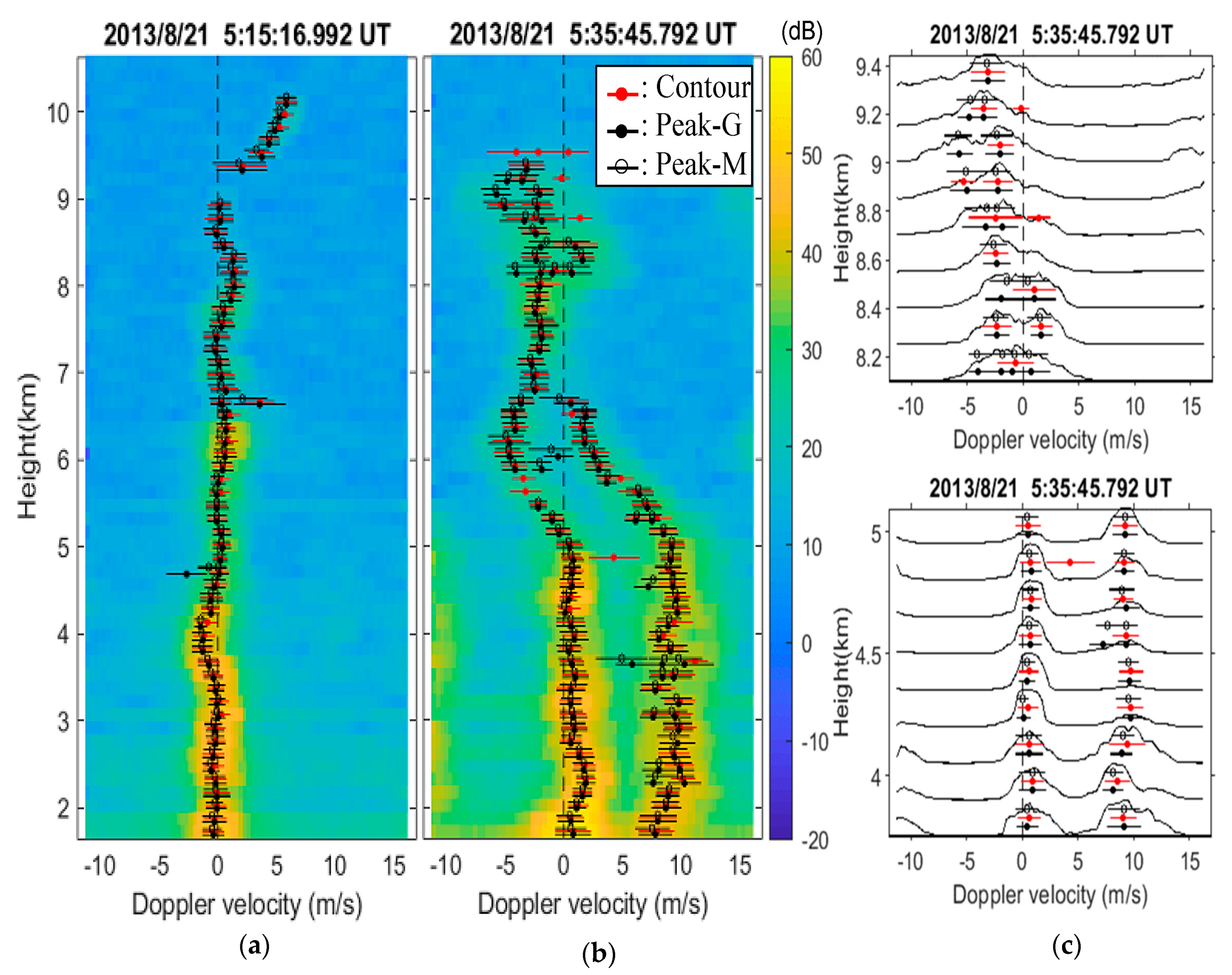
Figure 7a,b show two examples of Doppler spectra (coloured image) varying with height, which were calculated from 64-point FFT. Positive and negative Doppler velocities denote approaching and receding motions, respectively. The number of incoherent integrations of Doppler spectrum was 2, resulting in a duration of about 17 s for a Doppler spectrum. Notice that the positive Doppler range was extended to about 16 m/s, which exceeded the Nyquist Doppler velocity of about 11 m/s. The reason for such extension and the manner of extension can refer to the pre-processing described in Section 2.1.

Additionally, shown in Figure 7a,b are the Doppler velocities and the spectral widths of clear-air and precipitation echoes, which were estimated from the contour-based (marked in red) and peak-finding (marked in black) approaches, respectively. In Figure 7a, only the clear-air echoes were visible, while in Figure 7b the clear-air echoes (distributed around 0 m/s) and precipitation (characterized by salient positive Doppler velocities) were both present. As seen, the spectral parameters estimated by the two approaches were in agreement with each other generally, although there were discrepancies in them at some places. For a clearer inspection, the two panels in Figure 7c display the spectral power in curve for several sampling gates. As seen in the upper panel of Figure 7c, which shows the motion of clear air, the peak-finding approach determined four Doppler velocities (black dots) at the bottom gate, but the contour-based approach provided only one (red dot). Discrepancies in the calculated Doppler velocity can also be found at heights of around 8.4, 8.7, and 9.2 km, and at around 4.5 and 4.8 km (see the lower panel of Figure 7c). In view of this, further classification and grouping of these Doppler velocities are necessary for tracing respective Doppler profiles of clear air and precipitation; this is addressed in Section 4.

A statistical comparison between the spectral parameters obtained from the contour-based and peak-finding approaches is shown in Figure 8, in which V_C and SW_C are the Doppler velocity and spectral width of the contour-based approach, V_pg and SW_pg are the corresponding results of Gaussian fitting in the peak-finding approach, and V_pm and SW_pm denote the extra estimates using the moment method in the peak-finding approach. The histogram in each panel shows the distribution of the difference between the two spectral parameters, which is present between −2 and 2 m/s. As shown in Figure 8a for the clear-air echoes, the correlations between the two spectral parameters were very high, although the slope (~0.96) of the regression line for the values of SW_C and SW_pm (at the second row and middle column) was slightly lower than the others (close to 1). Note that, for the moment method executed in the peak-finding approach, the spectral lines within ±2 times of the Gaussian-fitted standard deviation were used in calculation, which included the spectral lines more than those in the Gaussian fitting method. As a result, the standard deviation (i.e., spectral width) estimated from the moment method could be slightly different from those of the Gaussian-fitting method. Such a situation was more observable under the conditions of strongly turbulent atmosphere and precipitation, as shown in Figure 8b. As seen, the slopes of the regression lines for the values of SW_C and SW_pg, SW_C and SW_pm, and SW_pg and SW_pm were smaller than those in Figure 8a, which reduced to about 0.98, 0.81, and 0.95, respectively. Moreover, the scatter dots in all panels of Figure 8b spread out more than in Figure 8a.

3.2. Spectral Parameters from Different FFT Numbers

Distributions of the spectral parameters calculated, respectively, by 32-, 64-, and 128-point FFT were shown in Figure 9, where only the calculations from the contour-based approach are present (V_C: Doppler velocity, SW_C: spectral width). For the clear-air echoes shown in Figure 9a, the three distributions of V_C and SW_C were relatively narrow, nearly invariant with height, and very close to each other, except for the height above ~8 km where the signal to noise ratio (SNR; indicated by thick, black profiling curve) was lower than 10 dB (10 dB is denoted by the dotted vertical line). Here, the SNR was calculated from the 64-point data length and self-normalized for presentation. By contrast, the distribution of V_C shown in Figure 9b varied highly with height, and SW_C was relatively broad.

A noticeable feature in the distributions of SW_C in Figure 9b was that the spectral width estimated from 128-point FFT (blue curve) was generally smaller than the other two. A detailed examination showed that in the environment of intense precipitation, the mean of spectral width became smaller (lager) if a FFT with more (less) data points was performed to generate the Doppler spectra, as shown in Figure 10. As seen in the left panel of Figure 10b, the mean of SW_C was the largest for 32-point FFT (black thin curve), and the smallest for 128-point FFT (blue curve) throughout the height. Such feature can be attributed to the smoothing effects on the spectrum caused by the windowing function in time domain, as well as the practice of incoherent integration in the spectral domain.

By contrast, the mean of SW_C shown in the left panel of Figure 10a, where the clear-air echoes dominated, were very close to each other. Above the height of ~4.5 km, however, the mean of SW_C from 32-point FFT was still slightly larger than the other two, and that from 128-point FFT was the smallest. On the other hand, irrespective of region 1 or region 2, the standard deviation of SW_C was nearly constant throughout the height, as shown in the right panels of Figure 10a and b, suggesting the robustness of the process in determination of spectral width. These results can be of help to advanced studies. For example, a careful investigation into the profiles of mean SW_C, the values increased slightly with height, especially observable in the results of 32- and 64-point FFT. This feature will be discussed further in Section 5.

3.3. Comparison between the Spectral Widths of Clear-Air and Precipitation Echoes

The spectral widths shown in Figure 10b were associated with both echoes of clear air and precipitation. It is of worth to find the difference between the spectral widths of clear air and precipitation when both echoes coexist. First, we categorized the spectral widths into two different groups in terms of Doppler velocity: between −3 and 3 m/s, and larger than 3 m/s. This is because that most of the Doppler velocities larger than 3 m/s were found to arise from precipitation echoes. Figure 11 shows the results calculated from the spectral widths (SW_C) for the radar echoes in region 2 of Figure 6a. In Figure 11a, all the outcomes of SW_C were used to estimate the mean (μ_SWc) and standard deviation (σ_SWc) of SW_C. It is apparent that the mean SW_C of precipitation echoes (red solid curve) was slightly larger than that of clear-air echoes (blue solid curve) below ~6 km; notice that strong precipitation occurred mainly below ~6 km in region 2 of Figure 6a, where the radar echoes were much larger than 10 dB. Even if the outcomes having the amplitudes larger than 0.5 or 0.8 (a normalized amplitude from the Gaussian fitting) were adopted, the mean SW_C of precipitation echoes were still larger than those of clear-air echoes below ~6 km, as demonstrated in Figure 11b and c. Moreover, the deviations of spectral widths (σ_SWc, dotted curves) were small for both echoes of clear air and precipitation. In view of this, the precipitation echoes indeed distributed over a broader range of Doppler velocity than the clear-air echoes. This result was expected because precipitation can be accelerated from rest to a terminal velocity of about 10 m/s in a vertical direction. Moreover, the falling velocities of precipitation may spread in a wider velocity interval due to different raindrop sizes. One more noticeable thing in Figure 11 is that only the clear-air echoes showed the feature of an increased spectral width with height (solid blue curve). This reveals the difference in spectral characteristics between clear-air and precipitation echoes.

4. Doppler Velocity Profiling

With the Gaussian-fitted Doppler velocities obtained from the two approaches proposed in Section 2, in the following we describe the process of tracing the respective Doppler velocities of clear air and precipitation through height. A brief flowchart describing the process is provided in Figure 1.

4.1. Tracing of Clear Air

Starting from the lowest sampling gate, the two Gaussian-fitted Doppler velocities within ±2 m/s and at the greatest significances that are determined, respectively, by the two proposed approaches, were averaged as an initial mean Doppler velocity (v₁) of clear-air motion. The respective amplitudes of the two Gaussian-fitted Doppler velocities were employed as the weights in the calculation of v₁. In case of no Gaussian-fitted Doppler velocity available in the first sampling gate, the second sampling gate was examined. This process might continue through several sampling gates until a value of v₁ was obtained. In case no v₁ was obtained from the lowest 15 sampling gates (the number is user defined), the value of 0 m/s was assigned to v₁.

Determination of mean Doppler velocity for the second sampling gate was based on v₁, i.e., by taking the Gaussian-fitted Doppler velocities within a velocity window between −v_dev and v_dev that centred on v₁, the weighted mean Doppler velocity was calculated as v₂. In the present calculation, v_dev =3 m/s. v₂ became the reference velocity of the next tracing in the third sampling gate. In a similar fashion, a Doppler velocity profile for clear air can be obtained. In practice, it happened occasionally that there was no reference velocity for the present sampling gate because the calculation failed in the preceding sampling gate due to the diagnosis of Doppler velocity shear (described below). In case of this, the tracing process continued searching for the existing mean Doppler velocity in the lower sampling gates. If no value was available in the 10 sampling gates lower than the present sampling gate, the searching process stopped.

In the tracing, the Doppler velocity shear is a crucial criterion. Assigning v_n, v_n−1, v_n−2, and v_n−3 to the mean Doppler velocities of the present and the lower three sampling gates, and v_shear to the threshold of Doppler velocity shear, v_n was discarded if |v_n − v_n−1| > v_shear or |v_n − v_n−2| > 1.5v_shear or |v_n − v_n−₃| > 1.5v_shear. When v_n was discarded, the Gaussian-fitted Doppler velocities used for estimate of v_n were regarded as the part of precipitation and retained for profile of precipitation. For clear air, the value of 2 m/s was given for v_shear. Use of these Doppler shear criteria in tracing can increase the reliability of the traced Doppler profile, although intermittent breaks in the profile may happen occasionally. It should be stated here that all values assigned for tracing are changeable, considering the atmospheric condition is variable. Once the tracing of clear-air motion is completed, the fitted Doppler velocities within −v_dev/2 and v_dev/2, centring on the mean Doppler velocities of the sampling gates, were discarded in the tracing of precipitation velocity described below.

4.2. Tracing of Precipitation

It is assumed that the Doppler speed of precipitation near the ground is larger than that of clear-air motion in the observation using a vertical radar beam. Therefore, the initial mean Doppler velocity (v₁) of precipitation was calculated from the fitted Doppler velocities larger than 3 m/s. In case of no v₁ obtained in the lowest 15 sampling gates, 5 m/s was assigned to v₁. The tracing was carried out with the same process as that for clear air. However, considering a wider range of Doppler velocities during the falling of precipitation, 3 m/s was given for the threshold of Doppler velocity shear (v_shear), which was larger than 2 m/s used for clear air. Notice here that the fitted Doppler velocities used for tracing the Doppler profile of clear air had been discarded and were not included in the calculation.

4.3. Results of Doppler Profiling

In total, 109 Doppler spectra were produced from the radar data shown in Figure 6. Readers can find more tracing results via the hyperlink in the Supplementary Materials provided in this article. Figure 12 exhibits several typical tracing results, where the black and red curves are the traced Doppler profiles of clear air and precipitation, respectively. Original Doppler spectra are displayed in the background. The panels Figure 12a,b are two examples dominated by clear-air echoes, showing the tracing was good, although the airplane echoes might interfere with the tracing slightly, e.g., around the height of 7 km. In the panel Figure 12c, one more profile (red curve) was traced for precipitation, showing the precipitation echoes occurred aloft and was much weaker than the clear-air echoes. More successful tracings for both clear air and precipitation are exhibited in the panels Figure 12d–k, in which the strong interferences around 2 km height in the panel Figure 12j were treated properly in the tracing and had been discarded in the profiling.

Two cases that were not traced completely are shown in the panels Figure 12l,m. As seen, the Doppler profiles of clear air broke around the height of 5 km and continued again since ~6 km. The echoes in the height interval of 5 and 6 km were traced as precipitation, and the weak precipitation echoes between 5 and 7 km and around 5 m/s, which were traced successfully in the panel Figure 12k, were not identified. This was partly due to a large variation in Doppler velocity around 5 km altitude, and partly owing to a mixture of clear-air and precipitation echoes, making the tracing difficult. The Doppler profile of clear air became continuous again later, as shown in panels Figure 12n,o.

The two events in panels Figure 12l,m show that a large wind shear within a short-range interval could cause the tracing to fail occasionally. In addition, it was sometimes difficult to distinguish the clear-air and precipitation echoes when both types of signals had the Doppler velocities close to each other. For the present data which were collected in a severely convective condition, only two events, i.e., the panels Figure 12l,m, out of 109 tracing results mistook the Doppler profiles of clear air and precipitation around 5 km altitude. In view of this, the success rate of tracing was really high. It is expected that the spectral parameters and the tracing process validated in this study can be of help to more scientific studies in the future. We provide an extended study in the following section for readers’ reference.

5. Observation Campaign of Convective Precipitation

As shown in Figure 6, dynamic echoes were present in a height range between about 7 and 10 km in region 2. From the Doppler spectra shown in Figure 12d–o, these echoes were characterized by very broad spectral width combined with intense upward air motion (sometimes larger than 5 m/s) and were identified as clear-air echoes rather than precipitation echoes. Moreover, we observed that these echoes were followed by the presence of precipitation echoes from the supercooled droplets between about 5.5 and 7 km (the temperature of 0 °C occurred at the height of about 5.7 km according to the rawinsonde data nearby; shown later). This feature seems to suggest that there existed hydrometeors in the height range of 7 and 10 km that were responsible for the formations of the supercooled droplets below 7 km. To verify this, the measurement of a dual-polarization microwave radiometer was investigated to study the properties of the targets responsible for the echoes observed by the VHF radar.

The dual-polarization microwave radiometer (model: RPG-4CH-DPR) was deployed on the campus of National Defence University (~200 m above sea level), which was located at about 13.52 km southeast of the Chung-Li VHF radar site (~140 m above sea level). The radiometer operated at two frequency bands (400 MHz each) centred on 18.7 GHz and 36.5 GHz, respectively. It can detect the thermal radiation emitted from water vapour, liquid water particles (raindrop, cloud droplet, and supercooled water particle), atmospheric molecules, and solid particles at vertical and horizontal polarizations and thereby measure the so-called brightness temperatures (Tb) at two orthogonal polarizations. However, the contributions from atmospheric molecules and solid hydrometeors are tiny and can be ignored, compared with those of water vapour and liquid water. The difference between the Tb of vertical and horizontal polarizations, i.e., vertical Tb—horizontal Tb, termed polarization difference (PD), can be used to determine the geometrical shape of liquid water particles. For a round liquid water particle, the PD will be very close to zero, and for a liquid water particle in a horizontally oblate shape, a negative PD is expected. In general, the bigger the liquid particle is, the flatter the liquid water particle will be, and a more negative value of PD is measured. In addition to PD, the four-channel measurements (two frequencies and two polarizations) can retrieve the total mass of liquid water (LWP, a path-integrated liquid water content above a unit surface area) and distinguish respective contributions of liquid water from cloud droplets and liquid raindrops (denoted LWC and LWR thereafter, respectively). More information and the physical background of the measurements with microwave radiometers can be found in the literature, e.g., [34,35,36,37,38,39]. Several key capabilities of the radiometer used in this study are range of the brightness temperature measurement 0–350 K with a precision of 0.05 K, integration time (or data resolution) 1 s, half power beam width (HPBW) of the antenna beam 10.25° with a sidelobe level less than −30 dBc and precision of PD measurement ± 0.25 K.

Compared with 18.7 GHz, the frequency of 36.5 GHz is more sensitive to smaller liquid water particles and corresponds to a thicker slant optical thickness [40], which can cover the height range above the melting layer. Therefore, the PD measurement from the frequency band of 36.5 GHz was examined for the purpose of this study. It is noteworthy that according to the study of Hou and Tsai [39] with the same radiometer, the positively linear relationship between brightness temperature and rain rate decreased gradually when the rain rate was higher than 20 mm/h, and became doubtful when the rain rate reached the value of about 60 mm/h. According to the rain rates at 05:00 and 06:00 UTC measured by the two rain gauges at Dasi and Bade, which are closer to the radiometer and also closer to the observational path of the radiometer, were 3.5 and 19.0 mm, and 6.5 and 17.0 mm, respectively, the two sets of rain rates were much smaller than the rain rate measured by the disdrometer at the VHF radar site. In view of these observations, we suppose that the measurements of the radiometer are still reliable. More descriptions of the radiometer and measurement characteristics can refer to Hou and Tsai [39], and Yeh et al. [41].

Figure 13 depicts the configuration of experimental setup. The VHF radar beam was transmitted vertically, and the antenna beam of the radiometer was steered to the northwest direction at an elevation and azimuth angles of 30° and 341.5°, respectively. Therefore, the observation zone of the radiometer at the distance of 13.52 km lay about 5 km to the east of the VHF radar site, and approximately in the height range between 6.33 and 9.57 km above the sea level of the VHF radar site. As a result, there was no overlapped field of view between the obliquely pointed radiometer beam and the vertically pointed VHF radar beam. Nevertheless, by taking account of finite beam widths, the separation of observational volumes between the radiometer and the VHF radar was less than 5 km in the height range of 6.33 and 9.57 km. A separation of 5 km was not a considerable distance for the convective structure examined later that covered a horizontal region of over ten kilometres. Therefore, it was justified to compare the concurrent measurements of convective precipitation aloft made by the VHF radar and the radiometer.

Figure 14a provides five consecutive maps of meteorological radar reflectivity, which were trimmed from those released by the Central Meteorological Bureau of Taiwan.

As shown, a strong front-like convective precipitation structure (or rainband), tilted in northwest-southeast direction, was moving from north to south at a phase speed of about 20 m/s. The rainband approached the VHF radar (black circle) and the radiometer (white circle) around 05:15 and 05:22 UTC, respectively, and left the VHF radar after 05:45 UTC approximately. The rainband was a strong convective structure, according to the large and prevailing upward Doppler velocities found in the VHF radar spectra shown in Figure 12d–n. In the meantime, the PD shown in Figure 14b increased from about −1.5 to around zero between 05:18 and 05:42 UTC and decreased quickly after 05:42 UTC, although the PD fluctuated during this time interval. Fluctuation of PD could be due to changes of axis ration and DSD of raindrops during updraft motion. According to previous research, the axis ratio and DSD of raindrops might be influenced by rain rates and winds [42,43]. In spite of this, the PD during 05:18 and 05:42 UTC was statistically larger than those before and after the rainband coverage, therefore it is reasonable to assume that the shape of liquid water particles varied mostly from horizontally oblate shape to almost round shape during the passage of the convective structure, which can thus be speculated to be caused by an uplift of liquid water particles in the convective structure, i.e., the liquid water particles got more round during uplift.

In addition to PD, the temporal variations of LWP, LWC, and LWR are shown in Figure 14c. LWP consists of the contributions of LWR, LWC, and water vapour. However, it is shown in Figure 14c that LWP, LWC, and LWR varied in accordance with each other and LWP was approximately the sum of LWC and LWR. In view of this, the contribution of water vapour to LWP was minor in the present event. Since LWP, LWC, and LWR decreased gradually and recovered from the valley between 5.24 and 5.36 h UTC, it implies a general decrease in liquid water content in the observation volume of the radiometer in this time period. As observed in Figure 14a, however, the rain band approached and covered the area between the VHF radar and radiometer during this time interval, and so the liquid water content was expected to increase gradually, not decrease. In view of this, the mechanism responsible for decrease in liquid water content is worthy of discussion. We supposed that an interaction of ice crystals, water vapour, and supercooled water particles above the melting layer could be the candidate of the cause, as discussed below.

According to the rawinsonde measurement at 06:00 UTC, conducted by the Pan-Chiao radiosonde station that was located at about 25 km east-northeast of the VHF radar, the temperatures of 0 °C, −10 °C and −20 °C appeared at the heights of around 5.7 km, 7.6 km and 9.2 km, respectively, as shown in Figure 15a. Thus, it signifies that in the absence of the vertical air motion, the compositions of the hydrometeors in the height ranges of 5.7 and 7.6 km, and 7.6 and 9.2 km were essentially dominated by supercooled water particles and the mixture of ice crystals and supercooled water particles in the cloud, respectively. However, in the presence of intense updraft, the updraft-carried water vapour and liquid water particles can significantly determine the growth of ice crystals and/or supercooled water particles above the 0 °C isotherm level. The so-called Bergeron effect will proceed to transfer water vapour from supercooled water particles to ice crystals due to the difference in relative humidity around supercooled water particles and ice crystals [44], leading to decrease of LWP. Because of the expense of supercooled water particles and/or water vapour during the Bergeron process, LWC and LWR decrease as well, as those happened around 05:30 UTC in Figure 14c. As the ice crystals become larger, their weights increase and finally cause them to fall. During the fall of ice crystals, a second process, coalescence or accretion, continue increasing the weights of the falling ice crystals. Coalescence during the fall of ice crystals is a process that the supercooled water particles collide and merge together, and then freeze on the surface of ice crystals [45,46], leading to the formation of graupel particles. The process of coalescence can decrease LWP, LWC, or LWR, too.

More evidences supporting the above-mentioned processes can be found in the VHF radar spectral parameters. As shown in Figure 12, very broad coverage of Doppler spectra (could be as large as 10 m/s) were observed in association with the updrafts in the height interval between about 7 and 10 km (e.g., Figure 12e–j). Broad Doppler spectra can be related to intense turbulence, or beam broadening effect from horizontal wind. As shown in Figure 15b, the rawinsonde measurement at 06:00 UTC revealed that the horizontal wind speed ranged mostly between 15 and 20 m/s below 10 km height, which contributed about 0.92–1.22 m/s to the spectral width (estimated from wind speed × sin(half-power-half-beamwidth 3.5°)). This interval of values was very close to the mean of SW_C shown in Figure 10a. In view of this, the beam broadening effect seemed to dominate the spectral width of clear-air echoes observed here, and the slight increment of spectral width along the height was thought to be due to the increase of horizontal wind. By contrast, the mean and standard deviation of SW_C in Figure 10b were obviously larger than that in Figure 10a, indicating a more turbulent condition or larger horizontal wind under precipitation circumstance. Assuming the horizontal wind speed increases to 30 m/s during the passage of convective structure, the beam broadening effect contributes about 1.83 m/s to the spectral width, which might tell the mean values of SW_C around 9 km height in Figure 10b (refer to the curves of 32- and 64-point FFT). Nevertheless, since the Doppler spectral coverage in the height interval between 7 and 10 km was quite broad in Figure 12e–j (could reach 10 m/s), there must be intense turbulences between 7 and 10 km in addition to incremental horizontal wind. Vertical motion induced by such intense turbulences can intensify the Bergeron effect and coalescence process.

Falling of ice crystals and graupel particles started from the height of about 7 km, as shown by the red curves in Figure 12d–k. When the ice crystals and graupel particles fall below 0 °C isotherm level, they start to melt and become wet. Therefore, it is expected that their backscatter will be about 5–15 dB larger than those above the 0 °C isotherm level [45,46]. Indeed, as shown in Figure 12e–j, a drastic increase in the radar backscatter of the falling ice crystals and graupel particles was about 5–10 dB in the height interval of 4–5 km, where was approximately below the 0 °C isotherm level. This was coincident with the theoretical and previous experimental results [47,48]. As ice crystals and graupel particles fall, their downward speeds are expected to increase. This feature was also observed clearly in Figure 12e–j, where the downward speeds increased to 10 m/s at around the height of 4 km. Moreover, variations in the profiles of atmosphere and precipitation were coherent when the convective condition prevailed in the time interval of Figure 12d–m. Based on this, it is evident that a convective atmosphere played a key role in the precipitation motion.

6. Conclusions

Two approaches have been developed in this study to identify the Doppler velocities of clear air and precipitation when both types of echoes coexist in the VHF radar spectra, i.e., contour-based and peak-finding processes. Initially, the two approaches provided a few contour centres and spectral peaks, and then grouping and sifting of these centres and peaks were processed to yield several mean locations of spectral humps that are more appropriate for use. Finally, Gaussian fitting with different fitting numbers was carried out for each mean location of spectral hump to provide several Gaussian curves. Among the qualified Gaussian curves, the one with the smallest standard deviation was assigned to the optimal outcome of that spectral hump, which was based on two considerations: (1) the beam broadening effect associated with horizontal wind exists commonly, and (2) the processes of smoothing and incoherent integration of spectra can broad the spectral width. Therefore, the spectral parameters (i.e., Doppler velocity and spectral width) estimated from such obtained outcomes are expected to be closer to the true spectral characteristics. The spectral parameters produced by the two approaches were consistent with each other generally, but discrepancy in them existed sometimes. In view of this, the outcomes of the two approaches were regarded as complementary results and have been cooperatively used to develop a process of Doppler profiling for treating a great amount of radar data more effectively.

To achieve the above-mentioned works, some parameters and criteria such as SNR, contour level, peak amplitude, separation of peaks, Doppler shear, and so on, have been considered. These parameters and criteria are adjustable. A strongly convective atmosphere with heavy precipitation and intense turbulence has been selected to test the identification approach and profiling process, showing about 98% of the tracings were acceptable and thereby validated the suitability of the parameters and criteria, at least, for the present radar observation. It is thus expected that these parameters and criteria are usable for a moderately varied atmosphere. More traced profiles can be found via the hyperlink attached with this article. Keeping these parameters and criteria adjustable makes the approach and process more flexible for identification and profiling of Doppler spectra in diversified conditions. Compared with many existing methods, the proposed approaches employ only basic and common data analysis techniques and utilize sifting and grouping processes for the spectral parameters. A future work can also include the outcomes of the already existed peak-finding methods to raise the accuracy of profiling results.

An application study of convective precipitation using the Doppler profile, radar echo power, and spectral parameter, retrieved from a rainy and strongly convective atmosphere during the period of a typhoon passage, has been made. This was achieved via the collaborative observation with a dual-polarization microwave radiometer. The measurements yielded by the radiometer, such as polarization difference of brightness temperature, total liquid water path, liquid water of cloud, and liquid water of rain, suggest the occurrences of Bergeron effect as well as coalescence process on formation of ice crystals and graupel particles above the height of the melting layer. This is the first time to present a collaborative study on this issue with VHF atmospheric radar and microwave radiometer, as far as we know.

Finally, it is worth mentioning that the FFT spectra with different raw data numbers (32, 64, and 128) were also examined in this study. Statistical characteristics of spectral width showed that the more the FFT number, the narrower the spectral width was. In addition, the mean spectral widths retrieved from 32 and 64 FFT numbers increased with altitude more evidently than that of 128 FFT number. The altitude-dependent spectral width could be a response of the beam broadening effect arising from a varied horizontal wind with height. Nevertheless, the altitudinal variation in spectral width was invisible in precipitation echoes. Moreover, the spectral widths of precipitation were generally larger than those of clear-air turbulence, showing the precipitation had a wider variation range of vertical velocity. All these consequences may be valid only for the present data but provide us with the motivation to carry out a more in-depth study with the retrieved spectral parameters in the future.