Abstract
Land-use regression (LUR) has emerged as a promising technique for air pollution modeling to obtain the spatial distribution of air pollutants for epidemiological studies. LUR uses traffic, geographic, and monitoring data to develop regression models and then predict the concentration of air pollutants in the same area. To identify the spatial distribution of nitrogen dioxide (NO2), benzene, toluene, and m-p-xylene, we developed LUR models in Pohang City, one of the largest industrialized areas in Korea. Passive samplings were conducted during two 2-week integrated sampling periods in September 2010 and March 2011, at 50 sampling locations. For LUR model development, predictor variables were calculated based on land use, road lengths, point sources, satellite remote sensing, and population density. The averaged mean concentrations of NO2, benzene, toluene, and m-p-xylene were 28.4 µg/m3, 2.40 µg/m3, 15.36 µg/m3, and 0.21 µg/m3, respectively. In terms of model-based R2 values, the model for NO2 included four independent variables, showing R2 = 0.65. While the benzene and m-p-xylene models showed the same R2 values (0.43), toluene showed a lower R2 value (0.35). We estimated long-term concentrations of NO2 and VOCs at 167,057 addresses in Pohang. Our study could hold particular promise in an epidemiological setting having significant health effects associated with small area variations and encourage the extended study using LUR modeling in Asia.
1. Introduction
Land-use regression (LUR) modeling is an accepted exposure assessment methodology, supported by numerous published models at local, country, and continental scales, for predicting the spatial distribution of ambient air pollutants and assessing long-term exposure to traffic-generated air pollution [1]. Regression methods are used to model pollutant concentrations measured at given sites on the basis of variables that characterize their surrounding land use, population density, and traffic patterns, as described elsewhere [2,3,4].
The development of geographical information system (GIS) offers the opportunity to predict pollutant concentrations on a fine spatial scale. LUR modeling is widely used in community health studies for capturing the smaller-scale variability because of the increasing ability of GIS to provide land-use data [5].
With geographic variables, such as traffic intensity, proximity to roadways, commercial and government areas, industrial area and point sources, population, and housing density (independent variables), a statistical model regresses measured values of a pollutant at sampling locations (the dependent variable). Air pollution levels are then predicted for any location, such as individual homes, using the parameter estimates derived from the regression model that mainly includes nitrogen dioxide (NO2) and particulate matter (PM10 and PM2.5) [4,6,7,8,9,10,11,12].
In the studies using the LUR method in Europe and North American contexts, only six have been investigated for volatile organic compounds (VOCs) [13,14,15,16,17,18].
Moreover, the applications of LUR in Asian countries have been performed using regulatory monitoring and measured data in Japan [19], China [12], and Mongolia [20].
The traffic patterns and land use in Pohang, Korea, are very complicated because the world’s third-largest steelmaker is located in the city. Therefore, it would be required to estimate the concentrations of air pollutants such as NO2 and VOCs using LUR modeling for epidemiologic studies.
This study, modeled with measured data, could contribute to the wide and extended use of LUR models in Korea, as well as other countries in Asia. The objectives of this research are to (1) provide the concentrations of NO2 and VOCs with long-term sampling methods, (2) predict the spatial distributions of NO2 and VOCs in the study area with LUR modeling, and (3) identify which air pollutants can be predicted most accurately in Pohang City. These LUR models of NO2 and VOCs would be useful for providing an exposure assessment tool for the epidemiologic studies of the adverse health impacts of outdoor air pollution. In this study, we provided the long-term NO2 and VOC concentrations for every location in Pohang City, Korea.
2. Materials and Methods
2.1. Study Area
The study area is Pohang City, located at 36°01′ N and 129°20′ W, North Gyeongsang Province, South Korea. It is bordered by the East Sea to the east and covers an area of 1127 km2. The 2009 population of Pohang was 509,475 persons, and the population density was 451.97 persons/km2. Pohang is one of the largest industrialized areas in Korea and mainly manufactures steel products (Figure 1).
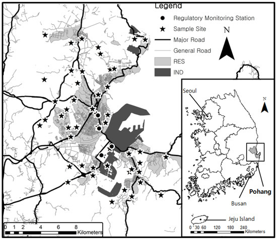
Figure 1.
Locations of sampling site in Pohang city, South Korea (RES: residential area; IND: industrial area).
2.2. Selection of Sampling Locations
Figure 1 shows the 50 locations of Pohang sampling sites including four regulatory monitoring stations, operated by the government, that are located in residential (2 sites) and industrial (2 sites) areas and used to monitor their exhausts. The regulatory monitoring stations in Pohang are designed to monitor compliance with regulatory standards. Although the location–allocation techniques [21] were not used, the monitoring sites were chosen based on a number of objective criteria to identify a spatial variability of NO2 and VOC. To investigate the spatial variability in the pollutant concentrations, 35 and 7 locations across the city were selected to ensure covering the residential area and nearby major roads, respectively. Since the focus was to capture the spatial trend of ambient pollution, especially where there were high numbers of residents, only 3 sites were located near or within the industrial area. Five sites were placed to provide information across the city, away from any noticeable local sources of importance, such as laneways or industrial areas. Consideration was provided to make sure the inclusion of all types of land use, such as road networks, industry, and residential settings.
2.3. Air Sampling and Analysis
Once the monitoring sites were selected, a NO2 passive sampler (Roshi Kaisha, Ltd., Tokyo, Japan [22]) and organic vapor samplers (3M, Saint Paul, MN, U.S.) were deployed for two 2-week integrated sampling periods to measure NO2 and VOC, respectively. The first sampling session included 50 locations monitored from 6 September to 20 September (henceforth “fall”) in 2010, and the second session was conducted between 15 March and 29 March (henceforth “spring”) in 2011 at the same 50 locations (Figure 1). Samplers were placed on lamp posts, utility poles, and street signs at a height of 2.5 m to prevent contamination and vandalism. Of the 50 samples, 4 were placed for duplicate samplings nearby the regulatory monitoring sites, and 5 field blanks in each session and pollutant were sampled. NO2, sampled by passive sampling badge, was analyzed by a UV spectrophotometer. Based on the recommendation of Lee et al. [23], an overall mass transfer coefficient of 0.10 cm/s was used. Analytical quality for the NO2 passive sampling badge was controlled by the blanks from each sampling location to explain the difference in sealing quality and lag time.
The 3M passive samplers were extracted with 2.0 mL of solvent and VOCs were determined by gas chromatography/mass selective detector (Shimadzu Corp., Kyoto, Japan). The results were corrected with laboratory blank, internal standard, and recovery. A more detailed description of the samplers and the performance can be found elsewhere [24,25,26,27].
Three VOCs (benzene, toluene, and m-p-xylene, henceforth “BTX”) were chosen for modeling. The number of measurements above minimum detection limits (MDL) for each pollutant and sampling session is shown in Table 1. All NO2 and BTX values were above the MDL (1 µg/m3 for NO2, 0.01 µg/m3 for BTX) except for 2 benzene and 6 m-p-xylene values in both sessions. The values below MDLs were replaced with MDL/√2 to provide a numerical result for all analyzed samples [28].

Table 1.
Number of observations above minimum detection limits (MDLs) for NO2, benzene, toluene, and m-p-xylene.
2.4. Temporal Trends and Adjustments
To account for the fact that measurements were made during two different sampling periods, and because our primary interest was in long-term (i.e., annual average) concentrations, NO2 data were converted to effective annual averages, as previously described elsewhere [11]. To account for any bias in the NO2 measurements, we planned to adjust NO2 concentrations based on the regulatory monitoring sites operated by the government (Figure 1). However, due to not providing government data during 2010–2011, we analyzed the average concentrations from 2005 to 2009 using the regulatory monitoring data for NO2 available from four sites in the GyeongSangbukdo Government Public Institute of Health and Environment. Then, we calculated the ratio of the annual average concentration to the relevant 2-week period (6 September–20 September 2020, 15 March–29 March 2021) and multiplied our measurements by the appropriate ratio to estimate the effective annual average. The two adjusted annual averages from each of the 50 locations were then averaged for LUR modeling. We could not adjust the BTX data because those were not provided by the regulatory monitoring sites. Therefore, we just averaged the two measurements in two sessions at each location. As a result, the BTX LUR models provide an assessment of relative concentrations across the city.
2.5. GIS Data
We generated variables in 5 categories and 20 subcategories to characterize the road length, land use, and population density in circular buffers with different radii around each sampling site (Table 2). All variables in each category were derived from a single spatial dataset in vector format.
Table 2.
Description of predictor variable categories for land-use regression model development.
The land-use data were obtained from the National Geographic Information Institute, an affiliated organization of the Ministry of Land, Transport and Maritime Affairs, Korea. In this study, land-use patterns included residential, industrial, open, commercial, government, and water variables. The population density in the city was obtained from Statistics Korea, based on the census data of 2007. The emission and point source data for BTX were obtained from the Pollutant Release and Transfer Registers (PRTR) Information System in the National Institute of Environmental Research, an affiliated organization of the Ministry of Environment, Korea. After converting the land use polygon into a raster file with 5 m pixels, we used Neighborhood Statistics, Spatial Analyst extension in ESRI’s ArcGis 9.3 (ESRI, Redlands, CA, USA) to sum the area of each land use type within the search radii based on a circular buffer (radii: 100, 200, 300, 500, 750, 1000, 1500, 2000 m) of each monitoring site.
The roads were classified into three categories: (1) major roads (MJR), including main city access roads and main intracity roads; (2) general roads (GEN), including secondary intercity roads; (3) minor or residential roads (MNR). These classifications were chosen according to the dominant use of the roads provided by the Ministry of Land, Transport, and Maritime Affairs, Korea. The road line was performed with the same approach in the land use polygon.
The Landsat ETM+ data were acquired from the Global Land Cover Facility (www.landcover.org, accessed on 13 July 2011). The advantage of using ETM+ data is its global coverage and free access. The scene for Pohang, Korea was at path-114/row-35 and captured on 10 September 2007. The ETM+ bands 1–5 and 7 were used to calculate the tasseled-cap brightness, greenness, and wetness [29], which were used to classify land cover types in Pohang. To facilitate the procedure of the LUR, all the individual images (30 m × 30 m) were resampled to have a spatial resolution of 5 m.
For population density, we used Calculate Density, Spatial Analyst extension in ESRI’s ArcGis 9.3 (ESRI, Redlands, CA, USA) to estimate the values within each search radius after converting census polygon to centroids and assigning each centroid the population count of the polygon from which it was derived (Table 2).
Eleven additional variables were included, which describe the geographic location of each site in terms of its elevation (ELEV), longitude (X), latitude (Y), distance to the city center (DCC), distance to the roads (DMJR, DGEN, and DMNR), distance from the ocean (DOC), and point sources for benzene, toluene, and xylene (DBP, DTP, and DXP), for a total of 140 potential predictors.
2.6. Land-Use Regression Model Development
While NO2 values showed the normal distribution, BTX values were log-normally distributed. Using an algorithm described by [4], we built models for NO2 and BTX: (1) Correlation coefficients between each potential predictor and the pollutants were calculated. (2) The predictors were ranked in each subcategory by the absolute value correlation. (3) Other variables with coefficients higher than 0.6 in the highest-ranking variables were eliminated. (4) All remaining variables were entered into a stepwise multiple linear regression. (5) To include only variables contributing at least 1% to the model R2 and coefficients consistent with a priori assumptions (e.g., positive coefficients for industrial land use variables and negative coefficients for open land use), the models were rerun as necessary.
2.7. Evaluation of the Developed Models
The models were evaluated based on the model-based R2 and root mean square error from a “leave-one-out” cross-validation. Each model was repeatedly parameterized on N-1 data points, where N is the total number of each pollutant in the selected sites, and then the concentration at the excluded site was predicted. Independent variables reserved in the models had to have a significant t-value (p < 0.05) and low collinearity, variance inflation factor (VIF < 2.0), with other retained variables. The surfaces of predicted NO2 and BTX concentrations were created by applying the coefficients of the predictive model equation and generating predicted surfaces with a 5 × 5 m resolution. Where the estimates exceeded 120% of the highest measured concentration, grid cell values were truncated. All geographic variables were calculated with ArcGIS 9.3 (ESRI, Redlands, CA, USA).
Statistical analyses were performed using SAS (Statistical Package for the Social Sciences, SAS Institute Inc., Cary, NC, USA) 9.2 for Windows. The correlations among measured air pollutants were analyzed by Spearman’s rank correlation test.
3. Results
3.1. Descriptive Statistics
Descriptive statistics for measured and temporally adjusted NO2 and BTX concentrations are shown in Table 3. With the duplicate samples, measurement precisions calculated as the standard deviation of duplicate differences divided by the square root of 2 were 1.88 µg/m3 for NO2, 0.13 µg/m3 for benzene, 0.37 µg/m3 for toluene, and 0.002 µg/m3 for m-p-xylene. The averaged mean concentrations of NO2, benzene, toluene, and m-p-xylene were 28.4 µg/m3 (SD = 7.5), 2.40 µg/m3 (SD = 1.13), 15.36 µg/m3 (SD = 5.20), and 0.21 µg/m3 (SD = 0.13), respectively. The mean value of NO2 in the fall session was significantly higher than that in spring, while the adjusted mean concentration (28.3 ± 7.5 µg/m3) of NO2 in 50 locations was lower than that (41.0 ± 6.2 µg/m3) of annual average from 4 regulatory monitoring sites. The mean values of benzene and toluene in the fall session were significantly higher than those in spring, while m-p-xylene showed the opposite result.
Table 3.
Statistical summary of measured NO2 and BTX, and temporally adjusted NO2 concentrations (unit: µg/m3).
Table 4 shows the correlation coefficients between pollutants. Benzene had significant correlations with NO2, toluene, and m-p-xylene.
Table 4.
Correlation coefficients between ambient NO2 and BTX compounds.
3.2. LUR Models
The final LUR models and modeled pollution maps are shown in Table 5 and Figure 2, respectively. In terms of model-based R2 values, the model for NO2 included four independent variables, showing the R2 = 0.65. While the benzene and m-p-xylene models showed the same R2 values (0.43), toluene showed lower R2 values (0.35). In NO2 and BTX model equations, the major road predictor (MJR) was commonly included, showing 2000 m buffer in NO2, 50 m buffer in benzene, 500 m buffer in toluene, and 300 m buffer in m-p-xylene. Additionally, industrial predictors (IND) were included in NO2 (2000 m buffer), benzene (500 m buffer), and toluene (2000 m buffer). “Leave-one-out” cross-validation R2 values for NO2, benzene, toluene, m-p-xylene were 0.56, 0.34, 0.26, and 0.33, respectively.
Table 5.
Final land-use regression models for NO2, benzene, toluene, and m-p-xylene.

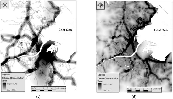
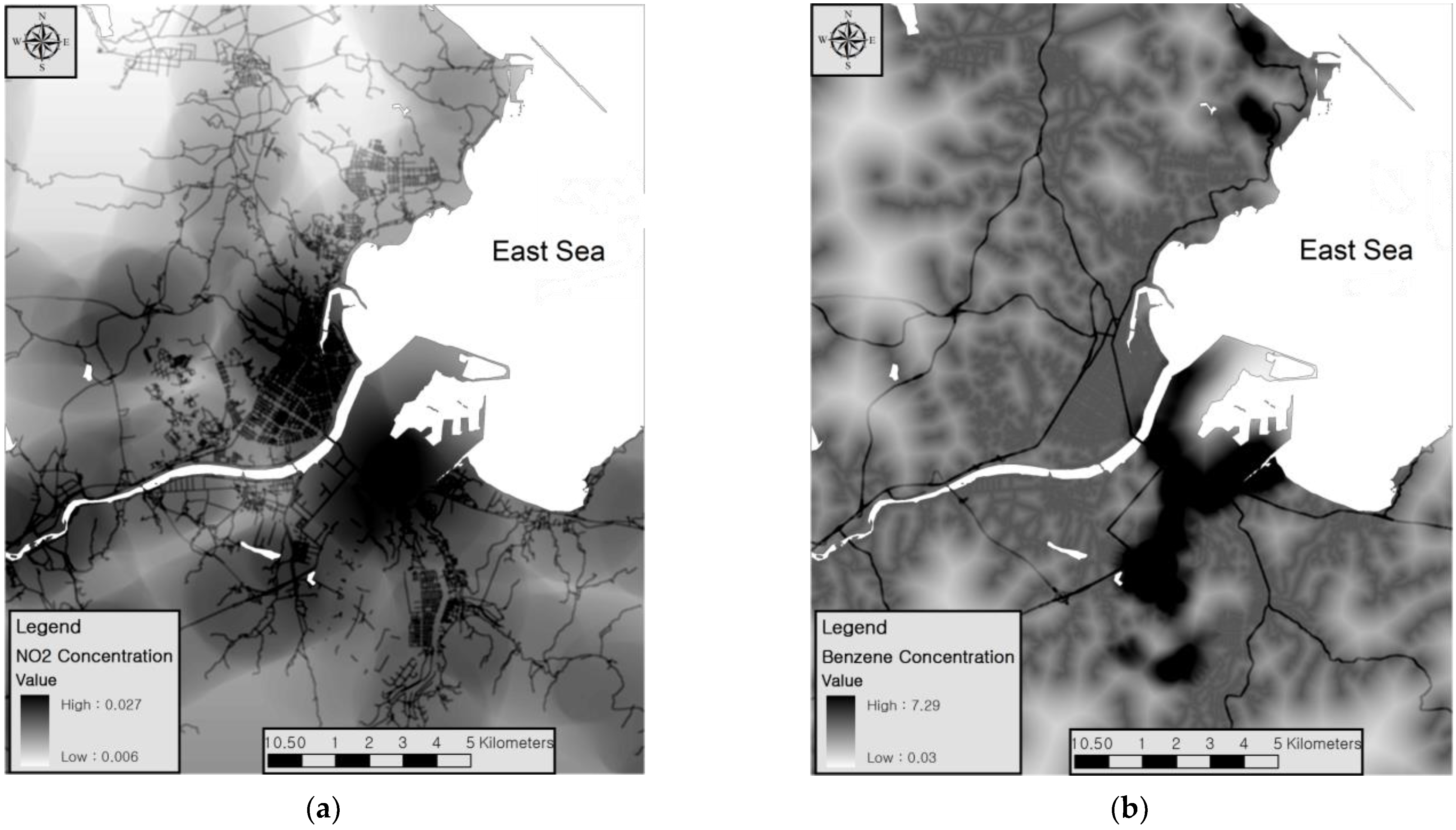
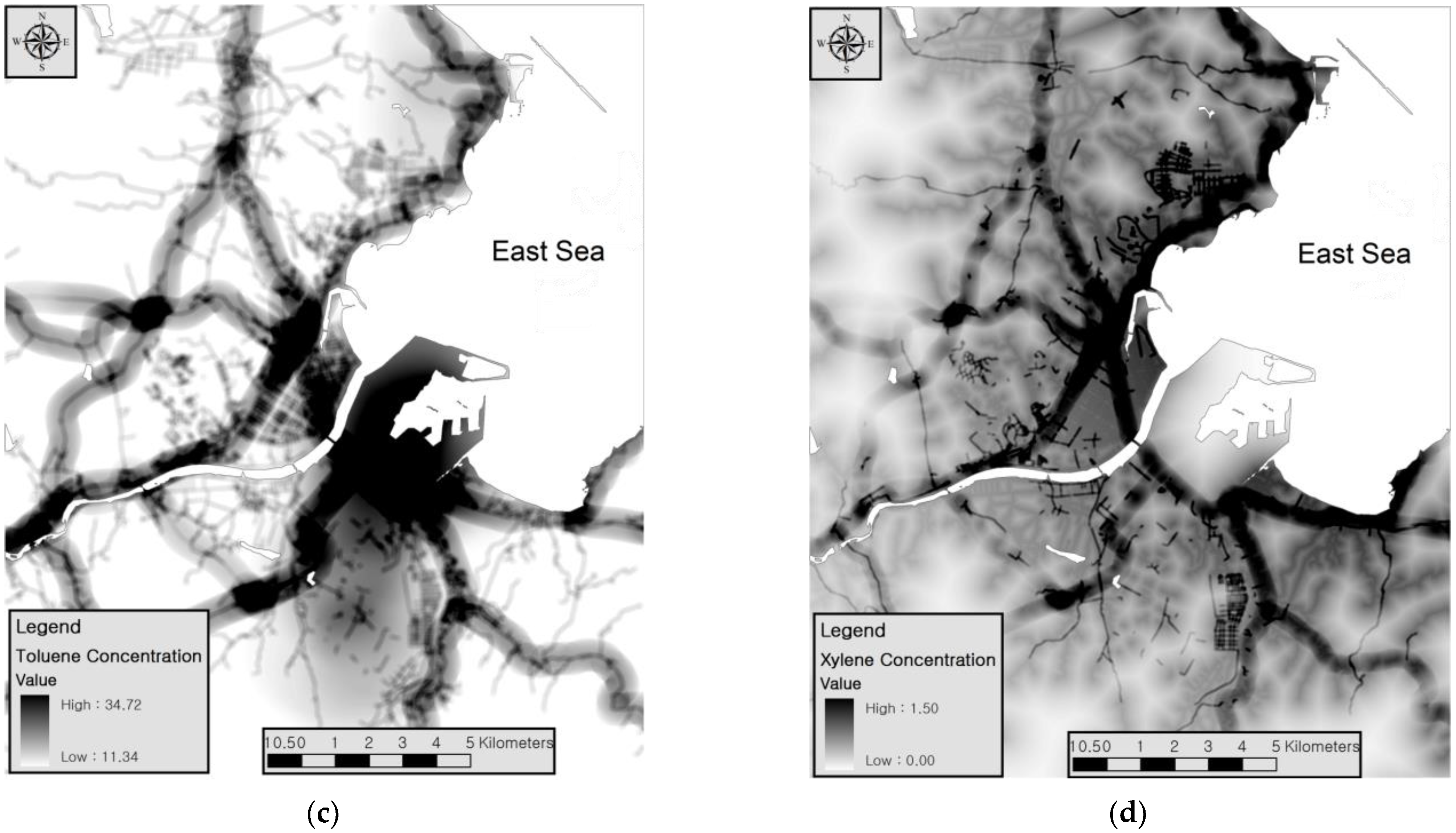
Figure 2.
Modeled concentrations (µg/m3) of NO2 (a), benzene (b), toluene (c), and m-p-xylene (d) in Pohang.
3.3. Estimation of VOC Concentrations at Locations
By applying the equation of the regression models on a 5 m cell basis to all locations in the city area, we modeled maps for NO2, benzene, toluene, and m-p-xylene concentrations (Figure 2) and then estimated long-term concentrations at 167,057 addresses in Pohang. These addresses contained 154,367 dwellings and 464,710 residents based on 2007 census data. The estimated air pollutant levels (not shown) of NO2 (20.7 µg/m3), benzene (1.46 µg/m3), toluene (12.13 µg/m3), m-p-xylene (0.17 µg/m3) in Pohang area were lower than measured data in sampling sites (Table 3).
4. Discussion
In this study, we developed LUR models for the estimation of air pollutants concentrations (NO2 and BTX) in Pohang, Korea by applying the measured data in 50 sampling locations. This study showed the NO2 concentration was properly estimated using the predictor variables, but BTX modeling had comparatively low R2.
In Table 3, the measured NO2 concentration was 28.4 µg/m3, ranging from 11.3 µg/m3 to 41.4 µg/m3 and lower than the annual NO2 average in Pohang regulatory monitoring stations. To remove bias introduced by seasonal trends in background concentrations [11], the measured NO2 values were corrected with adjusted factors of fall and spring, respectively to acquire the effective annual average.
The measured benzene concentrations (Table 3) in our study ranged from 0.41 to 6.08 µg/m3, with a mean value of 2.40 µg/m3, much lower than typically identified [30,31,32,33]. However, the values were similar to the measured data (1.4–2.7 µg/m3) reported by Baek et al. [34] for the same city, Pohang.
The correlation between NO2 and BTX species in this study (Table 4) showed slightly different coefficient ranges, compared with other studies in the US and Canada [35,36]. Our research had slightly low and narrow coefficient ranges (0.31–0.46) compared with those (0.53–0.89) reported in Toronto, Canada [35]. While the higher correlation ranges (0.78–0.99) resulted from the numerous petrochemical industries in the region [36], the lower correlation coefficients in this study may have been due to complicated NO2 and BTX sources from roads, residential, and industrial areas. The significant correlation between NO2 and benzene indicated that benzene was partially from traffic, considering other correlations among benzene, toluene, and m-p-xylene, presumably being from industrial areas.
As shown in Table 5, the R2 value for our NO2 model was 0.65. The highest R2 values of NO2 in the previous studies of Europe and North America were 0.77 in San Diego, United States [37] and 0.77 in Montreal, Canada [15], followed by 0.76 in Huddersfield, 0.73 in Sheffield, United Kingdom [3], 0.56 in Vancouver, Canada [4], 0.54 in Montreal, Canada [8], and 0.51 in Munich, Germany [10]. In Asia, the values of R2 are 0.74 and 0.61 in Tianjin, China [12], 0.54 in Shizuoka, Japan [19], and 0.74 in Ulaanbaatar, Mongolia [20]. Our R2 value was in the middle of the previous R2 values for the NO2 model. Our NO2 modeling had variables related to industrial areas, as well as traffic variables. The result may support the fact that the densely populated areas, areas located in the north, and industrial areas also have higher traffic lengths.
In Pohang, only four regulatory monitoring stations are deployed to control the air quality level for the purpose of compliance with air standards. Even though there was a reasonable result about R2 value in NO2 modeling [19] using regulatory air quality data, the modeling would be possible in the case of providing the monitoring stations that can gather background data, not affected by specific sources of air pollutants. Without monitoring stations being able to gather background levels and having enough numbers, there would be no other way other than directly measuring NO2 levels. Therefore, we selected the sampling sites located in the residential and industrial areas, including high traffic areas, and some locations to gather background data to cover the entire city.
On the other hand, R2 for the BTX models showed 0.43, 0.35, and 0.43 for benzene, toluene, and m-p-xylene, respectively. Moreover, their R2 were lower than those observed in similar studies (0.73 for benzene [38], 0.76 for toluene and 0.80 for benzene [13], 0.90 for BTEX [14], 0.74 for BTEX [16], 0.73 for benzene [15], and 0.72 and 0.71 for benzene and m-p-xylene (winter), respectively [18]. Nevertheless, some results in those studies showed similar R2, 0.46 for toluene [15], 0.49, 0.41, and 0.40 for benzene, toluene, and xylene (summer), respectively [18].
The “leave-one-out” procedure was conducted to evaluate the validity of the regression models. The resulting estimations were a root mean squared error (RMSE) of 4.3 µg/m3 for NO2, 0.24 µg/m3 for ln(benzene), 0.17 µg/m3 for ln(toluene), and 0.54 µg/m3 for ln(m-p-xylene), as shown in Table 5. The RMSE value for NO2 modeling in this study was similar to that in a previous study (4.5–4.7 µg/m3) [39,40].
Even though we tried to apply the remote sensing data such as brightness, greenness, and wetness as predictor variables in NO2 and BTX modeling, the remote sensing variables were not included in the final land-use regression model. Since the application of satellite remote sensing data in LUR modeling in recent years [16,38,41,42,43], modeling based on Landsat ETM+ data has provided a relatively easy and feasible way to improve exposure analysis in cases in which highly resolved traffic, road, and land-use data are unavailable.
In our LUR modeling study, on the other hand, we directly measured the NO2 and BTX levels with passive samplers to cope with the limitations of the regulatory monitoring data described above. The main encouragement of our LUR modeling is to bring effective tools that can extract reliable estimates of air pollutants concentrations for epidemiological study and risk assessment [4]. Therefore, according to spatial variability of the measured or regulatory monitored data, the appropriate process should be applied for extracting reliable estimates in LUR modeling.
In conclusion, our land-use regression models hold particular promise in epidemiological settings having significant health effects associated with small area variations. While the NO2 model appears to predict well, data limitations hampered our ability to gather all potentially useful predictors in BTX models. Further studies are needed on designing more detailed monitoring and modeling strategies for epidemiological studies of chronic health effects.
5. Conclusions
For the first time, we developed LUR models for the estimation of air pollutant concentrations for NO2, benzene, toluene, and m-p-xylene in Korea. The performance of the LUR model was comparable to that found in previous reports in Europe and North America as well as Asia. The major road predictor in all models was commonly included, and the industry predictor was also found in NO2, benzene, and toluene models. The application of this prediction model is a promising tool for the assessment of individual levels of exposure to traffic and industry-related air pollution. The results obtained from this study will be utilized as fundamental data for a predictive model to pertinently manage the level of urban air pollution.
Author Contributions
Conceptualization & methodology, H.-J.C. and K.-Y.K.; investigation, Y.-M.R., Y.-W.L. and Y.-J.L.; writing, H.-J.C. and K.-Y.K. All authors have read and agreed to the published version of the manuscript.
Funding
This research was funded by the Korea Institute of Planning and Evaluation for Technology in Food, Agriculture, and Forestry (IPET) through the Livestock Industrialization Technology Development Program, funded by the Ministry of Agriculture, Food and Rural Affairs (MAFRA) (Grant Number: 321089-05-1-HD030).
Institutional Review Board Statement
Not applicable.
Informed Consent Statement
Not applicable.
Conflicts of Interest
The authors declare no conflict of interest.
References
- Hoek, G.; Beelen, R.; de Hoogh, K.; Vienneau, D.; Gulliver, J.; Fischer, P.; Briggs, D. A review of land-use regression models to assess spatial variation of outdoor air pollution. Atmos. Environ. 2008, 42, 7561–7578. [Google Scholar] [CrossRef]
- Jerrett, M.; Arain, A.; Kanaroglou, P.; Beckerman, B.; Potoglou, D.; Sahsuvaroglu, T.; Morrison, J.; Giovis, C. A review and evaluation of intraurban air pollution exposure models. J. Expo. Sci. Environ. Epidemiol. 2004, 15, 185–204. [Google Scholar] [CrossRef] [PubMed]
- Sahsuvaroglu, T.; Arain, A.; Kanaroglou, P.; Finkelstein, N.; Newbold, B.; Jerrett, M.; Beckerman, B.; Brook, J.; Finkelstein, M.; Gilbert, N.L. A land use regression model for predicting ambient concentrations of nitrogen dioxide in Hamilton, Ontario, Canada. J. Air Waste Manag. Assoc. 2006, 56, 1059–1069. [Google Scholar] [CrossRef] [PubMed] [Green Version]
- Henderson, S.B.; Beckerman, B.; Jerrett, M.; Brauer, M. Application of land use regression to estimate long-term concentrations of traffic-related nitrogen oxides and fine particulate matter. Environ. Sci. Technol. 2007, 41, 2422–2428. [Google Scholar] [CrossRef] [PubMed]
- Burrough, P.A.; McDonnell, R.; Lloyd, C.D. Principles of Geographical Information Systems; Oxford University Press: Oxford, UK, 1998. [Google Scholar]
- Brauer, M.; Hoek, G.; van Vliet, P.; Meliefste, K.; Fischer, P.; Gehring, U.; Heinrich, J.; Cyrys, J.; Bellander, T.; Lewne, M. Estimating long-term average particulate air pollution concentrations: Application of traffic indicators and geographic information systems. Epidemiology 2003, 14, 228. [Google Scholar] [CrossRef] [PubMed]
- Briggs, D.J.; de Hoogh, C.; Gulliver, J.; Wills, J.; Elliott, P.; Kingham, S.; Smallbone, K. A regression-based method for mapping traffic-related air pollution: Application and testing in four contrasting urban environments. Sci. Total Environ. 2000, 253, 151–167. [Google Scholar] [CrossRef]
- Gilbert, N.L.; Goldberg, M.S.; Beckerman, B.; Brook, J.R.; Jerrett, M. Assessing spatial variability of ambient nitrogen dioxide in montreal, canada, with a land-use regression model. J. Air Waste Manag. Assoc. 2005, 55, 1059–1063. [Google Scholar] [CrossRef] [PubMed] [Green Version]
- Gilliland, F.; Avol, P.K.; Jerrett, M.; Dvonch, T.; Lurmann, F.; Buckley, T.; Breysse, P.; Keeler, G.; de Villiers, T.; McConnell, R. Air pollution exposure assessment for epidemiologic studies of pregnant women and children: Lessons learned from the centers for Children’s environmental health and disease prevention research. Environ. Health Perspect. 2005, 113, 1447. [Google Scholar] [CrossRef] [Green Version]
- Morgenstern, V.; Zutavern, A.; Cyrys, J.; Brockow, I.; Gehring, U.; Koletzko, S.; Bauer, C.P.; Reinhardt, D.; Wichmann, H.E.; Heinrich, J. Respiratory health and individual estimated exposure to traffic-related air pollutants in a cohort of young children. Occup. Environ. Med. 2007, 64, 8. [Google Scholar] [CrossRef] [PubMed] [Green Version]
- Poplawski, K.; Gould, T.; Setton, E.; Allen, R.; Su, J.; Larson, T.; Henderson, S.; Brauer, M.; Hystad, P.; Lightowlers, C. Intercity transferability of land use regression models for estimating ambient concentrations of nitrogen dioxide. J. Expo. Sci. Environ. Epidemiol. 2008, 19, 107–117. [Google Scholar] [CrossRef] [Green Version]
- Chen, L.; Bai, Z.; Kong, S.; Han, B.; You, Y.; Ding, X.; Du, S.; Liu, A. A land use regression for predicting NO2 and PM10 concentrations in different seasons in Tianjin region, China. J. Environ. Sci. 2010, 22, 1364–1373. [Google Scholar] [CrossRef]
- Carr, D.; von Ehrenstein, O.; Weiland, S.; Wagner, C.; Wellie, O.; Nicolai, T.; von Mutius, E. Modeling annual benzene, toluene, NO2, and soot concentrations on the basis of road traffic characteristics. Environ. Res. 2002, 90, 111–118. [Google Scholar] [CrossRef] [PubMed]
- Smith, L.; Mukerjee, S.; Gonzales, M.; Stallings, C.; Neas, L.; Norris, G.; Ozkaynak, H. Use of GIS and ancillary variables to predict volatile organic compound and nitrogen dioxide levels at unmonitored locations. Atmos. Environ. 2006, 40, 3773–3787. [Google Scholar] [CrossRef]
- Wheeler, A.J.; Smith-Doiron, M.; Xu, X.; Gilbert, N.L.; Brook, J.R. Intra-urban variability of air pollution in windsor, ontario—measurement and modeling for human exposure assessment. Environ. Res. 2008, 106, 7–16. [Google Scholar] [CrossRef] [PubMed]
- Aguilera, I.; Sunyer, J.; Fernandez-Patier, R.; Hoek, G.; Aguirre-Alfaro, A.; Meliefste, K.; Bomboi-Mingarro, M.T.; Nieuwenhuijsen, M.J.; Herce-Garraleta, D.; Brunekreef, B. NOx, NO2 and BTEX exposure in a cohort of pregnant women using land use regression modeling. Environ. Sci. Technol. 2008, 42, 815–821. [Google Scholar] [CrossRef] [PubMed]
- Su, J.G.; Brauer, M.; Ainslie, B.; Steyn, D.; Larson, T.; Buzzelli, M. An innovative land use regression model incorporating meteorology for exposure analysis. Sci. Total Environ. 2008, 390, 520–529. [Google Scholar] [CrossRef] [PubMed]
- Smith, L.A.; Mukerjee, S.; Chung, K.C.; Afghani, J. Spatial analysis and land use regression of VOCs and NO2 in Dallas, Texas during two seasons. J. Environ. Monit. 2011, 13, 999–1007. [Google Scholar] [CrossRef] [PubMed]
- Kashima, S.; Yorifuji, T.; Tsuda, T.; Doi, H. Application of land use regression to regulatory air quality data in Japan. Sci. Total Environ. 2009, 407, 3055–3062. [Google Scholar] [CrossRef] [PubMed]
- Allen, R.W.; Gombojav, E.; Barkhasragchaa, B.; Byambaa, T.; Lkhasuren, O.; Amram, O.; Takaro, T.K.; Janes, C.R. An assessment of air pollution and its attributable mortality in Ulaanbaatar, Mongolia. Air Qual. Atmos. Health 2011, 6, 137–150. [Google Scholar] [CrossRef] [PubMed] [Green Version]
- Kanaroglou, P.S.; Jerrett, M.; Morrison, J.; Beckerman, B.; Arain, M.A.; Gilbert, N.L.; Brook, J.R. Establishing an air pollution monitoring network for intra-urban population exposure assessment: A location-allocation approach. Atmos. Environ. 2005, 39, 2399–2409. [Google Scholar] [CrossRef]
- Yanagisawa, Y.; Nishimura, H. A badge-type personal sampler for measurements of personal exposure to NO2 and NO in ambient air. Environ. Int. 1982, 18, 235–242. [Google Scholar] [CrossRef]
- Lee, K.; Yanagisawa, Y.; Spengler, J.D.; Özkaynak, H.; Billick, I.H. Sampling rate evaluation of NO2 badge:(I) in indoor environments. Indoor Air 1993, 3, 124–130. [Google Scholar] [CrossRef]
- Yamada, E.; Kimura, M.; Tomozawa, K.; Fuse, Y. Simple analysis of atmospheric NO2, SO2, and O3 in mountains by using passive samplers. Environ. Sci. Technol. 1999, 33, 4141–4145. [Google Scholar] [CrossRef]
- Mukerjee, S.; Smith, L.A.; Norris, G.A.; Morandi, M.T.; Gonzales, M.; Noble, C.A.; Neas, L.M.; Ozkaynak, A.H. Field method comparison between passive air samplers and continuous monitors for VOCs and NO2 in El Paso, Texas. J. Air Waste Manag. Assoc. 2004, 54, 307–319. [Google Scholar] [CrossRef] [PubMed]
- Sather, M.E.; Slonecker, E.T.; Mathew, J.; Daughtrey, H.; Williams, D.D. Evaluation of ogawa passive sampling devices as an alternative measurement method for the nitrogen dioxide annual standard in El Paso, Texas. Environ. Monit. Assess. 2007, 124, 211–221. [Google Scholar] [CrossRef]
- Mukerjee, S.; Smith, L.A.; Johnson, M.M.; Neas, L.M.; Stallings, C.A. Spatial analysis and land use regression of VOCs and NO2 from school-based urban air monitoring in Detroit/Dearborn, USA. Sci. Total Environ. 2009, 407, 4642–4651. [Google Scholar] [CrossRef]
- Succop, P.A.; Clark, S.; Chen, M.; Galke, W. Imputation of data values that are less than a detection limit. J. Occup. Environ. Hyg. 2004, 1, 436–441. [Google Scholar] [CrossRef] [PubMed]
- Huang, C.; Wylie, B.; Yang, L.; Homer, C.; Zylstra, G. Derivation of a tasselled cap transformation based on landsat 7 at-satellite reflectance. Int. J. Remote Sens. 2002, 23, 1741–1748. [Google Scholar] [CrossRef]
- Adgate, J.L.; Eberly, L.E.; Stroebel, C.; Pellizzari, E.D.; Sexton, K. Personal, indoor, and outdoor VOC exposures in a probability sample of children. J. Expo. Sci. Environ. Epidemiol. 2004, 14, S4–S13. [Google Scholar] [CrossRef] [Green Version]
- Rappaport, S.M.; Kupper, L.L. Variability of environmental exposures to volatile organic compounds. J. Expo. Sci. Environ. Epidemiol. 2004, 14, 92–107. [Google Scholar] [CrossRef] [Green Version]
- Weisel, C.P.; Zhang, J.J.; Turpin, B.J.; Morandi, M.T.; Colome, S.; Stock, T.H.; Spektor, D.M.; Korn, L.; Winer, A.; Alimokhtari, S. Relationship of indoor, outdoor and personal air (RIOPA) study: Study design, methods and quality assurance/control results. J. Expo. Sci. Environ. Epidemiol. 2004, 15, 123–137. [Google Scholar] [CrossRef] [PubMed] [Green Version]
- Sexton, K.; Mongin, S.; Adgate, J.; Pratt, G.; Ramachandran, G.; Stock, T.; Morandi, M. Estimating volatile organic compound concentrations in selected microenvironments using time-activity and personal exposure data. J. Toxicol. Environ. Health Sci. Part A 2007, 70, 465–476. [Google Scholar] [CrossRef] [PubMed]
- Baek, S.O.; Kim, S.H.; Kim, M.H. Characterization of atmospheric concentration of volatile organic compounds in industrial areas of Pohang and Gumi cities. J. Environ. Toxicol. 2005, 20, 167–178. [Google Scholar]
- Beckerman, B.; Jerrett, M.; Brook, J.R.; Verma, D.K.; Arain, M.A.; Finkelstein, M.M. Correlation of nitrogen dioxide with other traffic pollutants near a major expressway. Atmos. Environ. 2008, 42, 275–290. [Google Scholar] [CrossRef]
- Pankow, J.F.; Luo, W.; Bender, D.A.; Isabelle, L.M.; Hollingsworth, J.S.; Chen, C.; Asher, W.E.; Zogorski, J.S. Concentrations and co-occurrence correlations of 88 volatile organic compounds (VOCs) in the ambient air of 13 semi-rural to urban locations in the United States. Atmos. Environ. 2003, 37, 5023–5046. [Google Scholar] [CrossRef]
- Ross, Z.; English, P.B.; Scalf, R.; Gunier, R.; Smorodinsky, S.; Wall, S.; Jerrett, M. Nitrogen dioxide prediction in southern california using land use regression modeling: Potential for environmental health analyses. J. Expo. Sci. Environ. Epidemiol. 2005, 16, 106–114. [Google Scholar] [CrossRef] [PubMed]
- Su, J.G.; Jerrett, M.; Beckerman, B.; Verma, D.; Arain, M.A.; Kanaroglou, P.; Stieb, D.; Finkelstein, M.; Brook, J. A land use regression model for predicting ambient volatile organic compound concentrations in Toronto, Canada. Atmos. Environ. 2010, 44, 3529–3537. [Google Scholar] [CrossRef]
- Briggs, D.J.; Collins, S.; Elliott, P.; Fischer, P.; Kingham, S.; Lebret, E.; Pryl, K.; Van Reeuwijk, H.; Smallbone, K.; Van Der Veen, A. Mapping urban air pollution using GIS: A regression-based approach. Int. J. Geogr. Inf. Sci. 1997, 11, 699–718. [Google Scholar] [CrossRef] [Green Version]
- Hoek, G.; Meliefste, K.; Brauer, M.; van Vliet, P.; Brunekreef, B.; Fischer, P.; Lebret, E.; Cyrys, J.; Gehring, U.; Heinrich, A. Risk Assessment of Exposure to Traffic-Related Air Pollution for the Development of Inhalant Allergy, Asthma and Other Chronic Respiratory Conditions in Children (TRAPCA). Final Report; IRAS University: Utrecht, the Netherlands, 2001. [Google Scholar]
- Su, J.G.; Brauer, M.; Buzzelli, M. Estimating urban morphometry at the neighborhood scale for improvement in modeling long-term average air pollution concentrations. Atmos. Environ. 2008, 42, 7884–7893. [Google Scholar] [CrossRef]
- Gao, L.N.; Tao, F.; Ma, P.L.; Wang, C.Y.; Kong, W.; Chen, W.K.; Zhou, T. A short-distance healthy route planning approach. J. Transp. Health 2022, 24, 101–114. [Google Scholar] [CrossRef]
- Ma, P.; Tao, F.; Gao, L.; Leng, S.; Yang, K.; Zhou, T. Retrieval of Fine-Grained PM2.5 Spationtemporal Resoultion Based on Multiple Machine Learning Models. Remote Sens. 2022, 14, 599. [Google Scholar] [CrossRef]
Publisher’s Note: MDPI stays neutral with regard to jurisdictional claims in published maps and institutional affiliations. |
© 2022 by the authors. Licensee MDPI, Basel, Switzerland. This article is an open access article distributed under the terms and conditions of the Creative Commons Attribution (CC BY) license (https://creativecommons.org/licenses/by/4.0/).