Abstract
Poor air quality is a major environmental concern worldwide, but people living in low- and middle-income countries are disproportionately affected. Measurement of PM2.5 is essential for establishing regulatory standards and developing policy frameworks. Low-cost sensors (LCS) can construct a high spatiotemporal resolution PM2.5 network, but the calibration dependencies and subject to biases of LCS due to variable meteorological parameters limit their deployment for air-quality measurements. This study used data collected from June 2019 to April 2021 from a PurpleAir Monitor and Met One Instruments’ Model BAM 1020 as a reference instrument at Alberta, Canada. The objective of this study is to identify the relevant meteorological parameters for each season that significantly affect the performance of LCS. The meteorological features considered are relative humidity (RH), temperature (T), wind speed (WS) and wind direction (WD). This study applied Multiple Linear Regression (MLR), k-Nearest Neighbor (kNN), Random Forest (RF) and Gradient Boosting (GB) models with varying features in a stepwise manner across all the seasons, and only the best results are presented in this study. Improvement in the performance of calibration models is observed by incorporating different features for different seasons. The best performance is achieved when RF is applied but with different features for different seasons. The significant meteorological features are PM2.5_LCS in Summer, PM2.5_LCS, RH and T in Autumn, PM2.5_LCS, T and WS in Winter and PM2.5_LCS, RH, T and WS in Spring. The improvement in R2 for each season (values in parentheses) is Summer (0.66–0.94), Autumn (0.73–0.96), Winter (0.70–0.95) and Spring (0.70–0.94). This study signifies selecting the right combination of models and features to attain the best results for LCS calibration.
1. Introduction
Air-quality monitoring is an integral part of the regulatory and management system of any region. It helps to assess the pollutant levels in the atmosphere concerning the ambient air-quality standards. In 2016, it was estimated that ambient outdoor air pollution caused 4.2 million premature deaths annually worldwide in both cities and rural areas [1]. Although poor air quality is a major environmental concern in most parts of the world, people living in low- and middle-income countries are affected disproportionately, with 91% of the 4.2 million premature deaths occurring in these regions [1,2]. This mortality is due to the exposure to fine particulate matter (PM2.5) as they are easily inhalable and cause chronic respiratory disease and cancers [3,4]. Measurement of PM2.5 in ambient air is essential for establishing regulatory standards and developing policy frameworks. Therefore, it is crucial that the air-quality measurements are spatiotemporally dense, economically feasible, and accurate [5]. Traditional monitoring instruments such as gravimetric method, beta attenuation monitor (BAM) and tapered element oscillating microbalance (TEOM) are expensive, have high operation and maintenance costs, and require highly skilled professionals to perform measurements. This limits their deployment, especially in areas that have significant spatial gradients of pollution concentration [6,7,8,9]. In the past decade, significant efforts have been made for the rapid development of low-cost sensors that enable inexpensive and dense spatial measurements of particle concentration [10,11,12,13]. However, the calibration dependencies and subject to biases of low-cost sensors for PM measurements are the challenges that must be addressed to use the data obtained from these sensors for quantitative assessment of air quality in a region [14,15].
Low-cost sensors are based on laser light-scattering technology (LLS) which means that the estimated concentration of particles depends on the factors such as aerosol composition, morphology, and meteorology that affect the interaction of light with particles [16,17,18,19,20]. Meteorological conditions such as relative humidity (RH) and temperature (T) are known to impact the performance and accuracy of LCS data [6,11,21,22]. Aerosol particles absorb water in high RH conditions, which changes their size, shape, refractive index and other properties, known as hygroscopic growth [23]. It affects the amount of light scattered by the particle and hence deviates from actual particle concentration. Additionally, PM measurements using regulatory-grade instruments (FRM/FEM) must be performed at specific temperature and humidity conditions (T: 20–23 °C, RH: 30–40%). However, LCS measures data in ambient conditions, which causes discrepancies in reported concentrations [14,24]. Studies have indicated significant overestimation of true PM2.5 mass when RH is high (>80%) [15,16,22]. It has been emphasized in the literature that the inclusion of RH and T for developing LCS calibration models is crucial as it improves the accuracy and can account for up to 17% and 7% variation in the PM2.5 measurement by LCS [6,11,25,26,27,28]. Giordano et al. [10] summarized the details of several studies to examine the effects of different parameters on the calibration of LCS data. However, other meteorological parameters such as wind speed (WS) and wind direction (WD) may contribute to the inaccuracy of LCS measurements. Chen et al. [25] developed an ML-based calibration method to study the effects of T, RH, WS, and WD on LCS particle measurements. Unfortunately, the effect of selecting different meteorological parameters on the calibration strategy of LCS remains unclear. Furthermore, seasonal variations in meteorological parameters are not considered, leading to inconsistent results for a larger data set. Meteorological parameters vary seasonally and impact the LCS performance in different degrees, which might be overlooked in the case of a general model. Additionally, including data from multiple seasons will skew the data distribution and affect the model performance [29]. So, to investigate the impact of seasonal variation on LCS performance, individual calibration models for each season should be developed and evaluated. Incorporating auxiliary features in the LCS calibration models can be beneficial but with varying effects. Including irrelevant features can trivialize the effect of major variables, increase the model complexity and is difficult to interpret at the expense of model performance [29,30]. So, features selection is a critical and inevitable step in the LCS calibration process [29]. Stepwise regression of LCS data with RH, T, WS and WD across seasons is implemented to understand the impact of each parameter on LCS performance and calibration strategy.
This paper investigates the (a) correlation between the PM2.5 data from Met One Instruments’ Model BAM 1020 (reference instrument) and the underlying size distribution of PurpleAir monitor (PAM) that is used in the apportionment of PM1, PM2.5 and PM10 (b) effect of meteorological parameters such as RH, T, WS and WD on performance and calibration of LCS using ML algorithms (c) impact of seasonal variation on performance and calibration of LCS. The ML algorithms used in this study are Random Forest (RF), Gradient Boosting (GB) and k-Nearest Neighbor (kNN). The meteorological parameters vary seasonally, and their impact on LCS performance is distinct, so features need to be selected appropriately for each season. This study attempts to identify the relevant meteorological parameters for each season that significantly affect the performance of LCS and should be included in the calibration. Case-wise comparison of predicted values from ML algorithms with the LCS and reference instrument measurements is performed, and the best results are presented. The approach for estimating the right combination of features and model for the best performance of LCS calibration models seasonally is discussed.
2. Materials and Methods
2.1. Data
The PurpleAir monitor (PAM) evaluated in this study measures PM1.0, PM2.5, PM10, RH and T. PAM uses Plantower PMS 5003, one of the most widely used LCS for measurement of PM. The data for PAM are freely available online and can be accessed at [31]. The data used in this study were gathered from PAM available at Edmonton (McIntyre), the capital city of Alberta, Canada (53.4860, −113.4643). The Met One Instruments’ Model BAM 1020 is used as a reference instrument to evaluate the PAM. The data for the reference instrument were gathered from Alberta Air Data Warehouse [32] for the station Edmonton McIntyre (53.4859, −113.4647), which is at a distance of 11 m from the PAM. The EPA colocation guidelines were followed while selecting the LCS for this study [33]. The WS and WD data were also obtained from Alberta Air Data Warehouse. This study focuses on data from 3 June 2019 to 30 April 2021. The data from PAM were available at an interval of 10 min and were resampled to obtain the hourly concentrations. Further details about PAM’s measurement and data can be found at [34,35] for reference instruments.
2.2. Methodology
Regression is a prominent statistical tool and is applied in various fields of science and technology. Regression attempts to understand the dependence of one variable on another through mathematical modeling [36,37]. It generally includes two real-valued variables known as dependent (y) and independent (x) variables. Regression analysis maps a mathematical function between the variables represented by y = f(x) + ε, where ε is the error [38,39]. When regression models have only one independent variable, they are known as univariate regression models. However, regression models can have more than one independent variable, in which case they are known as multi-regression models.
In this study, four different regression algorithms were applied for calibration of LCS, viz. multiple linear regression (MLR), Random Forest (RF), Gradient Boosting (GB) and k-Nearest Neighbor (kNN). MLR is a simple regression technique while RF, GB and kNN are ML algorithms. ML algorithms have been reported to improve the accuracy of LCS calibration models in the literature [11,40,41,42]. RF and GB are tree-based ensemble ML algorithms that construct numerous decision trees and integrate their outputs for prediction. The major difference between RF and GB is the approach of integrating the decision trees. RF implements a simple average on the prediction of individual trees, while GB performs a weighted average based on the performance of individual trees [43,44,45,46]. However, kNN is an ML algorithm that assumes that similar objects occur closer by and memorizes the training data. kNN does not formulate any theory about the data and solely averages out the value of occurrences closer to a new sample for prediction [45,46,47]. The details of these algorithms are available and described in detail in the literature [11,43,45,46,47,48].
Stepwise regression was conducted on the LCS data to understand the importance of feature selection. The features selected for regression were based on the present literature, which describes their effects on the data quality of LCS measurements [10,16,17,18]. The effect of RH on the calibration of PM2.5_LCS data due to the hygroscopic growth of particles is widely known [23]. However, the calibration of LCS data with RH and T has been studied widely due to the interdependency of these meteorological parameters [11,21,22,49]. More recently, researchers have studied the effects of WS and WD on LCS calibration [25]. For this reason, these two parameters were included in the regression of calibration PM2.5_LCS with RH and T. The algorithms, viz. MLR, RF, GB and kNN, were tested individually stepwise with varying features for all the seasons, and the best results were presented. The entirety of the data was segregated into four seasons, namely Summer (June, July, August), Autumn (September, October, November), Winter (December, January, February) and Spring (March, April, May) to conduct seasonal calibration of LCS at Alberta, Canada [49].
3. Results and Discussion
3.1. Season Wise Variation of Meteorological Features
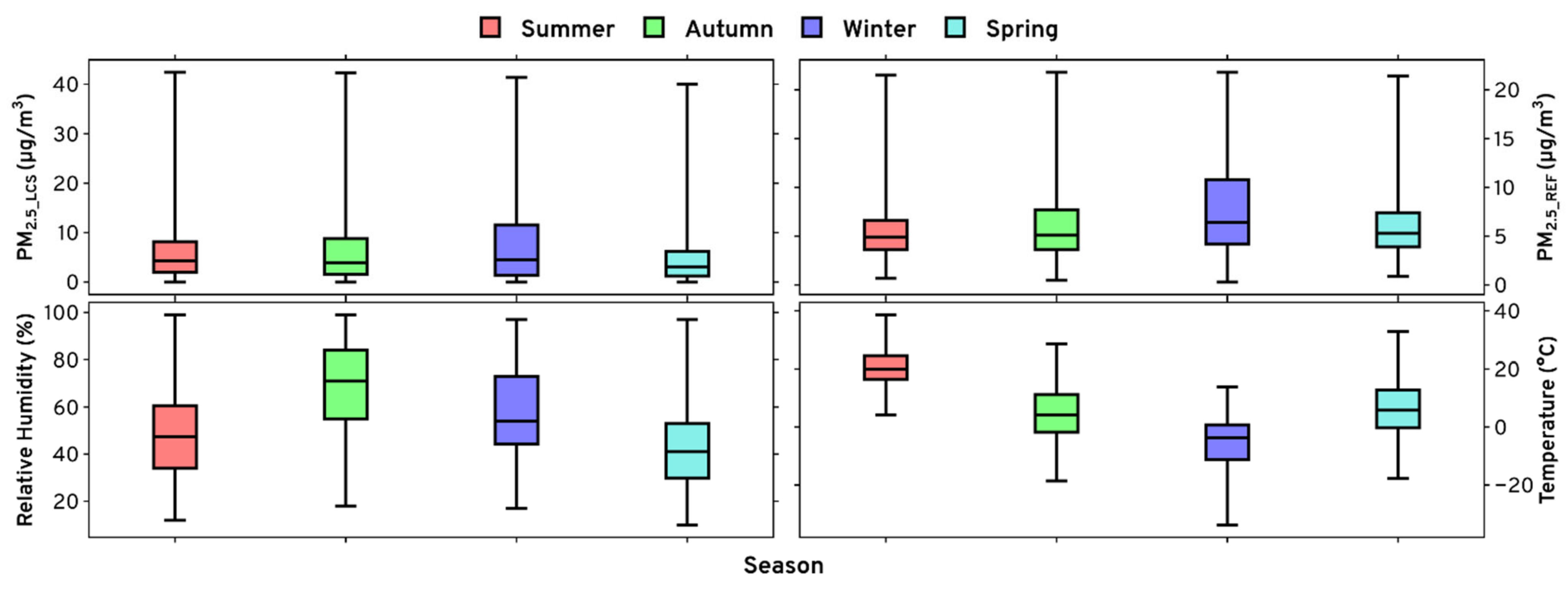
The PM mass concentrations recorded using LCS were influenced by variation in various meteorological parameters, as described in the earlier section. The meteorological parameters selected for this study included RH, T, WS and WD, which were used to calibrate the sensor PMX_LCS concentrations with PM2.5_REF. Table 1 shows a season-wise statistical summary of these variables. From the table, the variation in mean values of RH and T is noticeable, especially temperature (T) with an average value of 20.65 ± 5.87, 4.42 ± 9.04, −5.91 ± 9.08, 6.46 ± 9.24 °C in the Summer, Autumn, Winter and Spring season, respectively. The average value of RH is significantly higher in Autumn by 30%, 16% and 37% compared to Summer, Winter and Spring seasons, respectively. Wind speed (WS) has a negligible variation across seasons with a mean value of 7.46 ± 4.25, 7.30 ± 4.12, 6.66 ± 3.68, and 8.10 ± 4.48 m/s for Summer, Autumn, Winter and Spring season, respectively. The impact of wind direction (WD) on sensor performance is also studied. The major wind direction in Summer is South-East, while for Autumn, Winter and Spring, it is North, as can be seen in the wind rose plots presented in Figure S6 of the Supplementary Materials. Seasonal variation of these parameters is also shown using boxplots of PM2.5_LCS, PM2.5_REF, RH and T to understand the range of the variables in Figure 1. PM2.5_REF has a maximum value of 20 μg/m3 for all seasons, which is nearly half of the sensor recorded PM2.5 data as presented in histograms in Figures S2–S5 of the Supplementary Materials, which illustrates that PAM has a general tendency to over-predict irrespective of the season. It also indicates that these meteorological parameters vary seasonally and their impact on LCS performance is also distinctive. So, applying a general model might be inadequate for examining the impact of seasonal variation. This dictates the development and evaluation of calibration models for each season individually.

Table 1.
Statistical summary of the data used in the study.
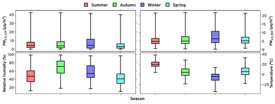
Figure 1.
Boxplot of variables for each season.
3.2. Comparison of PM1.0, PM2.5 and PM10 from LCS with PM2.5 from Reference Instrument
PAM uses a Plantower PMS5003 sensor, which is fundamentally a nephelometer as it operates on the principle of laser light-scattering technology. The sensor measures total light scattering, and the manufacturer’s proprietary algorithm apportions this to different size bins based on some underlying distribution and utilizes it to estimate the PM concentration (PM1.0, PM2.5 and PM10) based on the particle count. Therefore, LCS cannot truly resolve the sampled particles into different size fractions [50]. So, a comparison was conducted of PM1.0, PM2.5 and PM10 from LCS with each other and PM2.5 from reference instrument to identify which variable was closer to the actual PM2.5. The heatmap for the Pearson correlation coefficient (R) presented in Figure S1 of Supplementary Materials exhibits a strong correlation of PM2.5_LCS with PM1.0_LCS (0.99) and PM10_LCS (1). The regression analysis indicates that including PM1.0 and PM10 instead of PM2.5 measured from LCS does not provide significant variation in the results. The scatter plots and statistical performance of PM2.5_REF with PM1.0_LCS, PM2.5_LCS and PM10_LCS are presented in Figure 2a–c respectively, indicates approximately similar results for all the scenarios. The R2 between PM2.5_REF and PM2.5_LCS (0.7) is highest among all the cases, while RMSE (3.78) and MAE (2.71) are higher than PM1.0_LCS but lower than PM10_LCS. Due to this, PM1.0 and PM10 from LCS are not included in further calibration as the variation in the result is minimal. Only PM2.5 from LCS is used in further calibration tests.
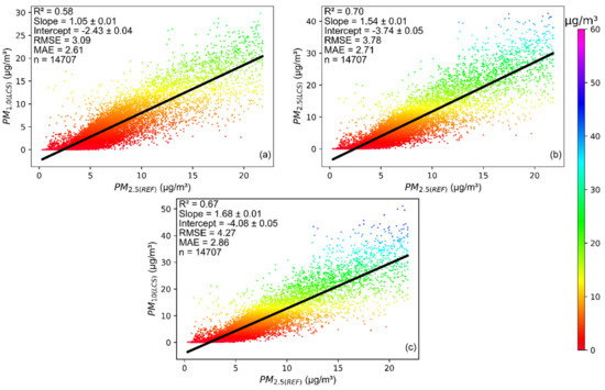
Figure 2.
Comparison between PM2.5_REF and (a) PM1.0_LCS; (b) PM2.5_LCS; and (c) PM10_LCS.
3.3. Effect of Meteorological Features and Seasons on LCS Calibration
PAM uses the Plantower PMS5003 sensor, a laser light-particle sensor that operates on Mie scattering theory [51]. Unlike the gravimetric method, where mass concentration is measured directly, LCS estimates the concentration based on the light scattered by the particles [22,52]. The light scattering is primarily a function of the particle size (d) and wavelength (λ) and can be classified into three regimes viz. Rayleigh (d << λ, d < 0.1 μm), Mie (d ≈ λ, 0.1 μm < d < 2 μm) and Optical (d >> λ, d > 2 μm) [17,53,54]. However, Mie scattering is a complex phenomenon that does not correspond only to particle size but depends on particle shape, morphology and refractive index as well [10]. Based on the scattered-light intensity from the particles in different size bins, the PM concentration is calculated by applying the confidential proprietary algorithm developed by the manufacturer. The Plantower PMS5003 sensor has six bins (0.3–10 μm) and applies Mie scattering theory on the entire range of particle sizes, which limits the true mass estimation of PM as a substantial portion of the particle sizes and number fall outside the scope of the Mie scattering regime. Another important aspect is the absence of particle count with a diameter < 0.3 μm while estimating the PM mass concentration, which excludes the contribution from sources such as sea salt, diesel engine, biogenic and other aerosols [55,56,57]. On the contrary, the reference instruments such as BAM and TOEM have 0.1 μm and 0.01 μm minimum detection limits, respectively. The light scattered by the particles is governed by the aerosol composition and morphology, porosity, shape and size distribution and meteorological conditions, which vary seasonally [17,18,19,22]. The variation in RH affects the optical and chemical properties of particles such as refractive index, density, etc., due to hygroscopic growth, which regulates the amount of light scattered. This causes inaccuracy in estimating the PM concentration due to seasonal variation in meteorological conditions, as discussed in Section 3.1, and so their impact on LCS performance will also be distinctive.
The source apportionment study conducted at Edmonton McIntyre, Alberta for 2009–2015 [58] reports that the major source of PM2.5 in Winter is secondary nitrate (3.14 µg/m3, 32.1%). However, secondary organic aerosol (SOA) is the major source in Summer (3.64 µg/m3, 51.7%), Spring (1.84 µg/m3, 20.5%) and Fall/Autumn (2.11 µg/m3, 28%). The contribution of secondary nitrate in Summer is almost negligible, while the contribution of traffic source varies from 0.96 µg/m3 (9.9%) in Winter to 1.57 µg/m3 (20.8%) in Autumn. Similarly, the contribution of biomass burning varies from 0.45 µg/m3 (6.1%) in Spring to 1.71 µg/m3 (17.5%) in Winter. This exhibits that the sources and their respective contributions vary seasonally, invariably altering the composition, particle size and distribution, hygroscopicity, density, refractive index, etc., which will fluctuate the scattered-light intensity. So, a single general model might suppress this information and will be incompetent to operate in varying conditions. In addition to this, using multi-season data in a single model can lead to the issue of imbalanced data, skewing the data distribution and affecting the model’s accuracy in the process [29].
However, before performing seasonal calibration the data were split into two parts, i.e., first year (June 2019–May 2020) and second year (June 2020–April 2021). The mean ± SD of PM2.5_LCS for the first and second year is 6.47 ± 7.10 µg/m3 and 6.11 ± 6.70 µg/m3, respectively. A statistical t-test indicated that the difference between the mean of the first and second year was insignificant (p < 0.05). The R2 between PM2.5_REF and PM2.5_LCS for the first and second year are 0.67 and 0.73, respectively. This suggests that there was little effect of aging or dust accumulation on the performance of LCS for two years at least. By applying MLR on these data by just taking PM2.5_LCS for calibration, R2 improved to 0.80 and 0.82 for the first and second year, respectively. So, the data are segregated seasonally based on the general trend of seasons occurring in Canada (Environment and Climate Change Canada, 2016) to examine the effect of seasonal variation on LCS performance. The seasonal calibration model development and results for each season are discussed below.
3.3.1. Summer
The scatter plot for the Summer season (before calibration) presented in Figure 3a indicates that the sensor-recorded data are in less agreement with the reference instrument as compared to the Autumn and Winter season, with R2, RMSE, and MAE values of 0.66, 3.37 and 2.21, respectively. MLR was applied for all variables in a stepwise manner to improve the sensor performance. The best results were obtained when MLR was applied on PM2.5_LCS and PM2.5_REF with an R2 value of 0.89 and a slope of 0.45, as presented in Table 2. The sensor performance had negligible improvement when other parameters were considered for calibration, which would only increase computational cost and model complexity. The statistical summary of sensor recorded data for the Summer season shows the highest average value of T (20.65 ± 5.87) and less RH (48.42 ± 18.02). It is inferred from the results that the sensor performance was degraded due to high temperature, which had a direct effect on RH in the ambient atmosphere. All three ML algorithms used in the study outperformed MLR with an improved R2 of 0.94, 0.91 and 0.91 for RF, GB and kNN, respectively. RF performed the best for Summer with a significant improvement in sensor performance compared to the results before calibration. The R2 improved by 0.28; RMSE and MAE decreased by 2.68 and 1.77, respectively.
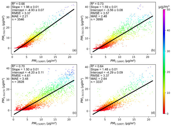
Figure 3.
Comparison between PM2.5_REF and PM2.5_LCS for the season of (a) summer; (b) autumn; (c) winter; and (d) spring.
Table 2.
Season-wise calibration of PM2.5_REF with PM2.5_LCS.
3.3.2. Autumn
The LCS-recorded data are in good agreement with the reference instrument for the Autumn season with an R2 value of 0.73 before calibration as presented in Figure 3b. MLR shows improvement in sensor performance with an R2, RMSE, MAE, and slope of 0.86, 1.48, 0.96 and 0.55, respectively. The best results were obtained when RH and T were considered for calibrating the sensor data with PM2.5_REF, as presented in Table 2. ML algorithms were used while considering the same meteorological features as in the case of MLR for calibration. RF, GB, and kNN performed better than MLR with R2 values of 0.96, 0.92 and 0.92, respectively.
3.3.3. Winter
MLR shows an improved R2 of 0.83 from before calibration R2 of 0.70 for the Winter season as shown in Figure 3c. T and WS were considered for calibration as they had significant slope values of −0.11 and −0.13, respectively. Since the winter season has a high mean value for RH, this means that the sensor overpredicted the PM2.5 mass concentration, which accounts for the negative slopes of T and WS in the calibration equation developed using MLR. Similar to other cases, ML algorithms gave better results with an R2 of 0.95, 0.89 and 0.89 for RF, GB and kNN, respectively. The train and test scores and other accuracy metrics are presented in Table 2.
3.3.4. Spring
The before calibration R2 is lowest for the Spring season (0.64) as presented in Figure 3d. The best results using MLR were obtained when RH, T and WS were included in the calibration for the Spring season. It is clear from the statistical summary of the data that WS was highest, and RH was lowest for the Spring season. MLR improved the R2 by 0.16, while RF, GB, and kNN improved the R2 value by 0.30, 0.23 and 0.22, respectively.
The comparison of PM2.5_LCS, PM2.5_REF and PM2.5_PRED from the best-case result for Summer, Autumn, Winter and Spring is presented in Figure S7a–d, respectively, in the Supplementary Materials. The figure exhibits that the predicted values are closer to the reference instrument compared to LCS measurements. The discussion on season-wise feature selection and calibration techniques to improve LCS performance shows the importance of choosing the right combination of suitable models and features to attain the best results. The relevant variables for LCS calibration vary for each season and have different weights. However, the weights obtained for parameters for each season (Table 1) are statistically significant (p < 0.05). The mean bias of seasonal models ranges from 2.82 in Summer to 5.61 in Spring, consistent with the values reported for PAM in the literature [59,60,61,62]. The mean bias can be reduced further by including chemical composition data, particle count below 0.3 µm, etc. The overall analysis determined that RF is the best-performing model with the inclusion of the correct features for each season.
The methodology and results presented in the study can be extrapolated to the other PAM sensors collocated with the sensor used in the study and reference instrument. PAM has a high precision [63,64], due to which the same models can be extrapolated if any other PAM sensor is collocated with the current sensor. The same methodology is applicable to other PM sensors from different manufacturers. However, the same models developed in the study cannot be directly applied to other sensors since the values of PM concentration reported by other sensors are dependent on their design, underlying distributions and laboratory calibration methods as these sensors are essentially nephelometers. In addition, particle binning and underlying algorithms to segregate particles in different size bins and PM estimation vary for each sensor. Additionally, the same approach can be applied to calibrate PM1.0 and PM10 by collocating the LCS with a reference instrument and obtaining the respective concentrations.
The study focuses on the calibration strategy by dividing the data collected from LCS and discusses the influence of selecting different meteorological parameters (feature selection) on LCS performance across seasons. The methodology adopted in the study can be applied to any data obtained from LCS collocated with a reference instrument, given that the data are sufficient to be divided into seasons for analysis. However, the same models generated for the LCS used in the study cannot be utilized for another LCS located in a different part of the world. The core idea of the study was to provide a hint towards the need for seasonal calibration of LCS instead of generating a global model because of seasonal variation of meteorological parameters. In the future, the proposed calibration strategy can be used on LCS located in different locations and may be helpful to provide better calibration results, particularly for locations with high variation of PM concentration, sources, and meteorological parameters.
4. Conclusions
A study was conducted to understand the impact of meteorological features and seasonal variation on the performance and calibration of low-cost sensors (LCS). The study used data collected from a PurpleAir Monitor, which operates on Plantower PMS5003 LCS and Met One Instruments’ Model BAM 1020 as a reference instrument at Alberta, Canada. Multiple Linear Regression (MLR), k-Nearest Neighbor (kNN), Random Forest (RF) and Gradient Boosting (GB) models were applied with varying features in a stepwise manner across all seasons. The meteorological features considered were relative humidity (RH), temperature (T), wind speed (WS) and wind direction (WD). Individual models for each season were developed for each algorithm and combination of meteorological parameters. The effect of meteorological parameters on calibration models varied seasonally. This study tried to identify the relevant meteorological parameters for each season that significantly affect the performance of LCS and should be included in the calibration while acknowledging the computational complexity. The best results were obtained for each season for features that were PM2.5_LCS in Summer; PM2.5_LCS, RH and T in Autumn; PM2.5_LCS, T and WS in Winter; and PM2.5_LCS, RH, T and WS in Spring. The R2 before and after calibration increased from 0.66, 0.73, 0.70 and 0.64 to 0.94, 0.96, 0.95 and 0.94 for Summer, Autumn, Winter and Spring seasons, respectively when RF was applied with the combination of features mentioned above. It is evident that RF is superior to other algorithms such as MLR, GB and kNN and is most suitable for LCS calibration. This study signifies selecting the right combination of models and features to attain the best results for LCS calibration.
Supplementary Materials
The following supplementary materials can be downloaded at: https://www.mdpi.com/article/10.3390/atmos13040587/s1. Figure S1: Pearson correlation coefficient between variables used in the study; Figure S2: Histogram of variables for the summer season; Figure S3: Histogram of variables for the autumn season; Figure S4: Histogram of variables for the winter season; Figure S5: Histogram of variables for the spring season; Figure S6: Wind rose plots for the season of (a) Summer, (b) Autumn, (c) Winter and (d) Spring; Figure S7: Comparison of PM2.5_REF, PM2.5_LCS and PM2.5_PRED for the season of (a) summer, (b) autumn, (c) winter and (d) spring.
Author Contributions
Conceptualization, V.K., V.M. and M.S.; Data curation, V.K. and V.M.; Funding acquisition, M.S.; Methodology, V.K., V.M. and M.S.; Project administration, M.S.; Resources, M.S.; Writing—original draft, V.K. and V.M.; Writing—review & editing, M.S. All authors have read and agreed to the published version of the manuscript.
Funding
This work has been supported by the Central Pollution Control Board as a part of the study “Pilot Study for Assessment of Reducing Particulate Air Pollution in Urban Areas by Using Air Cleaning System (sometimes called as Smog Tower)” (Grant no: RD/0120-CPCB000- 001). Partial support from the study “Application of Nanoparticles in ESP for Inactivation of Microorganisms and Degradation of VOCs for Air Purification” (Grant no: RD/0119- DST0000-048) is acknowledged.
Institutional Review Board Statement
Not applicable.
Informed Consent Statement
Not applicable.
Data Availability Statement
The data that support the findings of this study are available open and free to the public and can be accessed from PurpleAir’s open data portal for low-cost sensor and Alberta Air Data Warehouse for reference instruments.
Acknowledgments
The authors would like to thank and acknowledge PurpleAir’s open data portal and Alberta Air Data Warehouse for their efforts to make these data available for public use.
Conflicts of Interest
The authors declare no conflict of interest.
References
- World Health Organization. Ambient (Outdoor) Air Quality and Health. 2018. Available online: https://www.who.int/news-room/fact-sheets/detail/ambient-(outdoor)-air-quality-and-health/ (accessed on 7 September 2021).
- Gakidou, E.; Afshin, A.; Abajobir, A.A.; Abate, K.H.; Abbafati, C.; Abbas, K.M.; Abd-Allah, F.; Abdulle, A.M.; Abera, S.F.; Aboyans, V.; et al. Global, regional, and national comparative risk assessment of 84 behavioural, environmental and occupational, and metabolic risks or clusters of risks, 1990–2016: A systematic analysis for the Global Burden of Disease Study 2016. Lancet 2017, 390, 1345–1422. [Google Scholar] [CrossRef] [Green Version]
- Cohen, A.J.; Brauer, M.; Burnett, R.; Anderson, H.R.; Frostad, J.; Estep, K.; Balakrishnan, K.; Brunekreef, B.; Dandona, L.; Dandona, R.; et al. Estimates and 25-year trends of the global burden of disease attributable to ambient air pollution: An analysis of data from the Global Burden of Diseases Study 2015. Lancet 2017, 389, 1907–1918. [Google Scholar] [CrossRef] [Green Version]
- Yang, Y.; Ruan, Z.; Wang, X.; Yang, Y.; Mason, T.G.; Lin, H.; Tian, L. Short-term and long-term exposures to fine particulate matter constituents and health: A systematic review and meta-analysis. Environ. Pollut. 2019, 247, 874–882. [Google Scholar] [CrossRef] [PubMed]
- Adhikari, A. Introduction to spatiotemporal variations of ambient air pollutants and related public health impacts. In Spatiotemporal Analysis of Air Pollution and Its Application in Public Health; Li, L., Zhou, X., Tong, W., Eds.; Elsevier: Amsterdam, The Netherlands, 2020; pp. 1–34. [Google Scholar] [CrossRef]
- Rai, A.C.; Kumar, P.; Pilla, F.; Skouloudis, A.N.; DI Sabatino, S.; Ratti, C.; Yasar, A.-U.; Rickerby, D. End-user perspective of low-cost sensors for outdoor air pollution monitoring. Sci. Total Environ. 2017, 607–608, 691–705. [Google Scholar] [CrossRef] [PubMed] [Green Version]
- Le, T.-C.; Shukla, K.K.; Chen, Y.-T.; Chang, S.-C.; Lin, T.-Y.; Li, Z.; Pui, D.Y.; Tsai, C.-J. On the concentration differences between PM2.5 FEM monitors and FRM samplers. Atmos. Environ. 2020, 222, 117138. [Google Scholar] [CrossRef]
- Ayers, G.; Keywood, M.; Gras, J. TEOM vs. manual gravimetric methods for determination of PM2.5 aerosol mass concentrations. Atmos. Environ. 1999, 33, 3717–3721. [Google Scholar] [CrossRef]
- Noble, C.A.; Vanderpool, R.W.; Peters, T.M.; McElroy, F.F.; Gemmill, D.B.; Wiener, R.W. Federal Reference and Equivalent Methods for Measuring Fine Particulate Matter. Aerosol Sci. Technol. 2001, 34, 457–464. [Google Scholar] [CrossRef]
- Giordano, M.R.; Malings, C.; Pandis, S.N.; Presto, A.A.; McNeill, V.; Westervelt, D.M.; Beekmann, M.; Subramanian, R. From low-cost sensors to high-quality data: A summary of challenges and best practices for effectively calibrating low-cost particulate matter mass sensors. J. Aerosol Sci. 2021, 158, 105833. [Google Scholar] [CrossRef]
- Kumar, V.; Sahu, M. Evaluation of nine machine learning regression algorithms for calibration of low-cost PM2.5 sensor. J. Aerosol Sci. 2021, 157, 105809. [Google Scholar] [CrossRef]
- Karagulian, F.; Barbiere, M.; Kotsev, A.; Spinelle, L.; Gerboles, M.; Lagler, F.; Redon, N.; Crunaire, S.; Borowiak, A. Review of the Performance of Low-Cost Sensors for Air Quality Monitoring. Atmosphere 2019, 10, 506. [Google Scholar] [CrossRef] [Green Version]
- Kumar, P.; Morawska, L.; Martani, C.; Biskos, G.; Neophytou, M.K.-A.; DI Sabatino, S.; Bell, M.; Norford, L.; Britter, R. The rise of low-cost sensing for managing air pollution in cities. Environ. Int. 2015, 75, 199–205. [Google Scholar] [CrossRef] [PubMed] [Green Version]
- Malings, C.; Tanzer, R.; Hauryliuk, A.; Saha, P.K.; Robinson, A.L.; Presto, A.A.; Subramanian, R. Fine particle mass monitoring with low-cost sensors: Corrections and long-term performance evaluation. Aerosol Sci. Technol. 2019, 54, 160–174. [Google Scholar] [CrossRef]
- Liu, H.-Y.; Schneider, P.; Haugen, R.; Vogt, M. Performance Assessment of a Low-Cost PM2.5 Sensor for a near Four-Month Period in Oslo, Norway. Atmosphere 2019, 10, 41. [Google Scholar] [CrossRef] [Green Version]
- Barkjohn, K.J.; Bergin, M.H.; Norris, C.; Schauer, J.J.; Zhang, Y.; Black, M.; Hu, M.; Zhang, J. Using Low-cost sensors to Quantify the Effects of Air Filtration on Indoor and Personal Exposure Relevant PM2.5 Concentrations in Beijing, China. Aerosol Air Qual. Res. 2020, 20, 297–313. [Google Scholar] [CrossRef]
- Hagan, D.H.; Kroll, J.H. Assessing the accuracy of low-cost optical particle sensors using a physics-based approach. Atmos. Meas. Tech. 2020, 13, 6343–6355. [Google Scholar] [CrossRef] [PubMed]
- Crilley, L.R.; Shaw, M.; Pound, R.; Kramer, L.J.; Price, R.; Young, S.; Lewis, A.C.; Pope, F.D. Evaluation of a low-cost optical particle counter (Alphasense OPC-N2) for ambient air monitoring. Atmos. Meas. Tech. 2018, 11, 709–720. [Google Scholar] [CrossRef] [Green Version]
- Di Antonio, A.; Popoola, O.A.M.; Ouyang, B.; Saffell, J.; Jones, R.L. Developing a Relative Humidity Correction for Low-Cost Sensors Measuring Ambient Particulate Matter. Sensors 2018, 18, 2790. [Google Scholar] [CrossRef] [Green Version]
- Castell, N.; Dauge, F.R.; Schneider, P.; Vogt, M.; Lerner, U.; Fishbain, B.; Broday, D.; Bartonova, A. Can commercial low-cost sensor platforms contribute to air quality monitoring and exposure estimates? Environ. Int. 2017, 99, 293–302. [Google Scholar] [CrossRef]
- Bai, L.; Huang, L.; Wang, Z.; Ying, Q.; Zheng, J.; Shi, X.; Hu, J. Long-term field Evaluation of Low-cost Particulate Matter Sensors in Nanjing. Aerosol Air Qual. Res. 2020, 20, 242–253. [Google Scholar] [CrossRef]
- Badura, M.; Batog, P.; Drzeniecka-Osiadacz, A.; Modzel, P. Evaluation of Low-Cost Sensors for Ambient PM2.5 Monitoring. J. Sensors 2018, 2018, 5096540. [Google Scholar] [CrossRef] [Green Version]
- Lee, A.K.Y.; Ling, T.Y.; Chan, C.K. Understanding hygroscopic growth and phase transformation of aerosols using single particle Raman spectroscopy in an electrodynamic balance. Faraday Discuss. 2008, 137, 245–263. [Google Scholar] [CrossRef] [PubMed]
- U.S. Environmental Protection Agency (EPA). Monitoring PM2.5 in Ambient Air Using Designated Reference or Class I Equivalent Methods. 2016. Available online: https://www3.epa.gov/ttnamti1/files/ambient/pm25/qa/m212.pdf (accessed on 28 December 2021).
- Chen, C.-C.; Kuo, C.-T.; Chen, S.-Y.; Lin, C.-H.; Chue, J.-J.; Hsieh, Y.-J.; Cheng, C.-W.; Wu, C.-M.; Huang, C.-M. Calibration of Low-Cost Particle Sensors by Using Machine-Learning Method. In Proceedings of the 2018 IEEE Asia Pacific Conference on Circuits and Systems (APCCAS), Chengdu, China, 26–30 October 2018; pp. 111–114. [Google Scholar] [CrossRef]
- Lee, H.; Kang, J.; Kim, S.; Im, Y.; Yoo, S.; Lee, D. Long-Term Evaluation and Calibration of Low-Cost Particulate Matter (PM) Sensor. Sensors 2020, 20, 3617. [Google Scholar] [CrossRef] [PubMed]
- Lin, Y.; Dong, W.; Chen, Y. Calibrating Low-Cost Sensors by a Two-Phase Learning Approach for Urban Air Quality Measurement. Proc. ACM Interact. Mob. Wearable Ubiquitous Technol. 2018, 2, 1–18. [Google Scholar] [CrossRef]
- Zheng, T.; Bergin, M.H.; Johnson, K.K.; Tripathi, S.N.; Shirodkar, S.; Landis, M.S.; Sutaria, R.; Carlson, D.E. Field evaluation of low-cost particulate matter sensors in high- and low-concentration environments. Atmos. Meas. Tech. 2018, 11, 4823–4846. [Google Scholar] [CrossRef] [Green Version]
- Liang, L. Calibrating low-cost sensors for ambient air monitoring: Techniques, trends, and challenges. Environ. Res. 2021, 197, 111163. [Google Scholar] [CrossRef]
- Fang, X.; Bate, I. Using multi-parameters for calibration of low-cost sensors in urban environment. In Proceedings of the International Conference on Embedded Wireless Systems and Networks (EWSN), Uppsala, Sweden, 20–22 February 2017. [Google Scholar]
- PurpleAir. Real-Time Air Quality Map | PurpleAir. 2021. Available online: https://www.purpleair.com/map (accessed on 19 June 2021).
- Alberta Government. Ambient Data Download. 2021. Available online: https://airdata.alberta.ca/reporting (accessed on 20 June 2021).
- U.S. Environmental Protection Agency (EPA). How to Evaluate Low-Cost Sensors by Collocation with Federal Reference Method Monitors. 2018. Available online: https://www.epa.gov/sites/default/files/2018-01/documents/collocation_instruction_guide.pdf (accessed on 21 February 2022).
- PurpleAir. Using PurpleAir Data. 2021. Available online: https://docs.google.com/document/d/15ijz94dXJ-YAZLi9iZ_RaBwrZ4KtYeCy08goGBwnbCU/edit (accessed on 3 September 2021).
- Alberta Government. Alberta Air Data Warehouse. 2021. Available online: https://www.alberta.ca/alberta-air-data-warehouse.aspx (accessed on 25 September 2021).
- Rawlings, J.O.; Pantula, S.G.; Dickey, D.A. Applied Regression Analysis: A Research Tool; Springer: New York, NY, USA, 1998. [Google Scholar]
- Mendenhall, W.; Sincich, T. A Second Course in Statistics: Regression Analysis; Pearson: London, UK, 2014. [Google Scholar]
- Kroese, D.P.; Botev, Z.I.; Taimre, T.; Vaisman, R. Data Science and Machine Learning: Mathematical and Statistical Methods; CRC Press, Taylor & Francis Group: New York, NY, USA, 2019. [Google Scholar]
- Zaki, M.J.; Meira, W. Data Mining and Machine Learning: Fundamental Concepts and Algorithms; Cambridge University Press: Cambridge, UK, 2020. [Google Scholar]
- Wang, Y.; Du, Y.; Wang, J.; Li, T. Calibration of a low-cost PM2.5 monitor using a random forest model. Environ. Int. 2019, 133, 105161. [Google Scholar] [CrossRef]
- Wang, W.-C.V.; Lung, S.-C.C.; Liu, C.-H. Application of Machine Learning for the in-Field Correction of a PM2.5 Low-Cost Sensor Network. Sensors 2020, 20, 5002. [Google Scholar] [CrossRef]
- Wijeratne, L.O.; Kiv, D.R.; Aker, A.R.; Talebi, S.; Lary, D.J. Using Machine Learning for the Calibration of Airborne Particulate Sensors. Sensors 2019, 20, 99. [Google Scholar] [CrossRef] [Green Version]
- Sutton, C.D. Classification and Regression Trees, Bagging, and Boosting. In Handbook of Statistics; Elsevier: Amsterdam, The Netherlands, 2005; Volume 24, pp. 303–329. [Google Scholar] [CrossRef] [Green Version]
- Bishop, C.M. Pattern Recognition and Machine Learning; Springer: New York, NY, USA, 2006. [Google Scholar]
- Hastie, T.; Tibshirani, R.; Friedman, J. The Elements of Statistical Learning, Second Edition: Data Mining, Inference, and Prediction; Springer: New York, NY, USA, 2009. [Google Scholar]
- Yang, X.-S. Introduction to Algorithms for Data Mining and Machine Learning; Elsevier: Amsterdam, The Netherlands, 2019. [Google Scholar]
- Kuhn, M.; Johnson, K. Applied Predictive Modeling; Springer: New York, NY, USA, 2013. [Google Scholar]
- Jagatha, J.V.; Klausnitzer, A.; Chacón-Mateos, M.; Laquai, B.; Nieuwkoop, E.; van der Mark, P.; Vogt, U.; Schneider, C. Calibration Method for Particulate Matter Low-Cost Sensors Used in Ambient Air Quality Monitoring and Research. Sensors 2021, 21, 3960. [Google Scholar] [CrossRef]
- Environment and Climate Change Canada. Temperature Change in Canada. 2016. Available online: https://www.canada.ca/en/environment-climate-change/services/environmental-indicators/temperature-change.html (accessed on 23 July 2021).
- Tryner, J.; L’Orange, C.; Mehaffy, J.; Miller-Lionberg, D.; Hofstetter, J.C.; Wilson, A.; Volckens, J. Laboratory evaluation of low-cost PurpleAir PM monitors and in-field correction using co-located portable filter samplers. Atmos. Environ. 2019, 220, 117067. [Google Scholar] [CrossRef]
- Plantower. PMS5003 Datasheet. 2019. Available online: https://docs.smartcitizen.me/assets/datasheets/pms5003/PTQ3004-2015%20PMS5003%20series%20data%20manual%20English_SLT_V1.0K.pdf (accessed on 16 March 2022).
- He, M.; Kuerbanjiang, N.; Dhaniyala, S. Performance characteristics of the low-cost Plantower PMS optical sensor. Aerosol Sci. Technol. 2019, 54, 232–241. [Google Scholar] [CrossRef]
- Seinfeld, J.H.; Pandis, S.N. Atmospheric Chemistry and Physics: From Air Pollution to Climate Change; Wiley: Hoboken, NJ, USA, 2016. [Google Scholar]
- Gramsch, E.; Oyola, P.; Reyes, F.; Vásquez, Y.; Rubio, M.A.; Soto, C.; Pérez, P.; Moreno, F.; Gutiérrez, N. Influence of Particle Composition and Size on the Accuracy of Low Cost PM Sensors: Findings From Field Campaigns. Front. Environ. Sci. 2021, 9, 527. [Google Scholar] [CrossRef]
- Feng, L.; Shen, H.; Zhu, Y.; Gao, H.; Yao, X. Insight into Generation and Evolution of Sea-Salt Aerosols from Field Measurements in Diversified Marine and Coastal Atmospheres. Sci. Rep. 2017, 7, srep41260. [Google Scholar] [CrossRef] [PubMed]
- Tomasi, C.; Lupi, A. Primary and Secondary Sources of Atmospheric Aerosol. In Atmospheric Aerosols: Life Cycles and Effects on Air Quality and Climate Tomasi; Fuzzi, S., Kokhanovsky, A., Eds.; Wiley: Weinheim, Germany, 2016; pp. 1–86. [Google Scholar] [CrossRef]
- Wihersaari, H.; Pirjola, L.; Karjalainen, P.; Saukko, E.; Kuuluvainen, H.; Kulmala, K.; Keskinen, J.; Rönkkö, T. Particulate emissions of a modern diesel passenger car under laboratory and real-world transient driving conditions. Environ. Pollut. 2020, 265, 114948. [Google Scholar] [CrossRef] [PubMed]
- Bari, A.; Kindzierski, W.B. Fine particulate matter (PM2.5) in Edmonton, Canada: Source apportionment and potential risk for human health. Environ. Pollut. 2016, 218, 219–229. [Google Scholar] [CrossRef] [PubMed]
- Sayahi, T.; Butterfield, A.; Kelly, K.E. Long-term field evaluation of the Plantower PMS low-cost particulate matter sensors. Environ. Pollut. 2019, 245, 932–940. [Google Scholar] [CrossRef]
- Ardon-Dryer, K.; Dryer, Y.; Williams, J.N.; Moghimi, N. Measurements of PM2.5 with PurpleAir under atmospheric conditions. Atmos. Meas. Tech. 2020, 13, 5441–5458. [Google Scholar] [CrossRef]
- Jiang, Y.; Zhu, X.; Chen, C.; Ge, Y.; Wang, W.; Zhao, Z.; Cai, J.; Kan, H. On-field test and data calibration of a low-cost sensor for fine particles exposure assessment. Ecotoxicol. Environ. Saf. 2021, 211, 111958. [Google Scholar] [CrossRef]
- Zimmerman, N. Tutorial: Guidelines for implementing low-cost sensor networks for aerosol monitoring. J. Aerosol Sci. 2021, 159, 105872. [Google Scholar] [CrossRef]
- Feenstra, B.; Papapostolou, V.; Hasheminassab, S.; Zhang, H.; Der Boghossian, B.; Cocker, D.; Polidori, A. Performance evaluation of twelve low-cost PM2.5 sensors at an ambient air monitoring site. Atmos. Environ. 2019, 216, 116946. [Google Scholar] [CrossRef]
- Stavroulas, I.; Grivas, G.; Michalopoulos, P.; Liakakou, E.; Bougiatioti, A.; Kalkavouras, P.; Fameli, K.; Hatzianastassiou, N.; Mihalopoulos, N.; Gerasopoulos, E. Field Evaluation of Low-Cost PM Sensors (Purple Air PA-II) under Variable Urban Air Quality Conditions, in Greece. Atmosphere 2020, 11, 926. [Google Scholar] [CrossRef]


Publisher’s Note: MDPI stays neutral with regard to jurisdictional claims in published maps and institutional affiliations. |
© 2022 by the authors. Licensee MDPI, Basel, Switzerland. This article is an open access article distributed under the terms and conditions of the Creative Commons Attribution (CC BY) license (https://creativecommons.org/licenses/by/4.0/).