Abstract
Haze level evaluation is highly desired in outdoor scene monitoring applications. However, there are relatively few approaches available in this area. In this paper, a novel haze level evaluation strategy for real-world outdoor scenes is presented. The idea is inspired by the utilization of dark and bright channel prior (DBCP) for haze removal. The change between hazy and haze-free scenes in bright channels could serve as a haze level indicator, and we have named it DBCP-I. The variation of contrast between dark and bright channels in a single hazy image also contains useful information to reflect haze level. By searching for a segmentation threshold, a metric called DBCP-II is proposed. Combining the strengths of the above two indicators, a hybrid metric named DBCP-III is constructed to achieve better performance. The experiment results on public, real-world benchmark datasets show the advantages of the proposed methods in terms of assessment accuracy with subjective human ratings. The study is first-of-its-kind with preliminary exploration in the field of haze level evaluation for real outdoor scenes, and it has a great potential to promote research in autonomous driving and automatic air quality monitoring. The open-source codes of the proposed algorithms are free to download.
1. Introduction
In application scenarios like city surveillance and autonomous driving, high quality videos without haze are desired. However, in the real world, heavy haze weather accounts for a large proportion of outdoor scenes, which seriously affects the normal work of monitoring-related applications. One of the solutions is to adopt the haze level evaluation (HLE) technique. Assessing the degree of haze through video or picture is a useful aid on many occasions. For example, for self-driving cars, if the visibility is severely influenced by heavy haze, precise evaluation results will trigger the alarm to warn the driver immediately, which helps to guarantee people’s safety. Another instance comes from air quality monitoring. In hard natural features like deserts or mountaintops, it is usually difficult to install air quality inspection devices at the observation spot. HLE results could reflect extremely bad weather through remote surveillance videos, which is an effective substitute for traditional device-based air quality monitoring techniques.
Despite its great significance and wide application prospects, HLE technology has received little attention from researchers, and there are few studies on this topic. The closest approach is haze image quality assessment (IQA). However, current IQA methods are not suitable for HLE problem for three reasons. First, they might belong to a different IQA category. It is well known that the most famous IQA metric is the SSIM index [1] which aims to evaluate image quality using structural differences between an original image and its degraded counterpart. Although the SSIM method and its improved versions are widely used [2,3,4,5], they are not suitable for haze level assessment because these methods need reference images. Apparently, for haze images captured in real outdoor scenes, there exist no original haze-free images to be compared with. Second, traditional IQA metrics usually deal with degraded images that have suffered from channel transmission [1,6,7,8,9], which might undermine the inherent statistical distributions in natural scenes [10,11,12,13]. However, there is no report indicating that this kind of statistic destruction is observed in haze images. Third, evaluating the haze level of original pictures and assessing the quality of dehazed images are two different things. In recent years, an upsurge of research appeared on quality evaluation of haze removal pictures [14,15,16,17,18,19,20,21,22]. Since haze images could be turned into dehazed ones by various dehazing methods, the visual differences between original and dehazed pictures could be compared and serve as the performance criteria of haze removal algorithms. Again, the task of quality assessment for dehazed images is quite different from that of HLE. For HLE tasks, an objective index needs to be found to accurately reflect the hazy degree in the scene, whereas for dehazing evaluation more factors (e.g., noises introduced by haze removal algorithms) need to be considered. Although dehazing algorithms could remove haze visually, extra artifacts are possible to be introduced through the haze removal operation. This is why two criteria, i.e., visibility index and realness index, are respectively established in [22] to reflect the two different dehazing effects.
To further demonstrate the differences, two groups of pictures are compared in Figure 1. Obviously, the range of hazy degrees in the dehazed images are much smaller than those in the real natural haze images. Additionally, the images in the top row all look natural and real, while comparatively, the bottom dehazed images look visually different in terms of realness. Furthermore, the visibility in the real haze images is more like a global concept covering the whole region, whereas in the dehazed pictures the visibility is region dependent. Therefore, more effective methods need to be explored to assess haze level in real outdoor scenes.
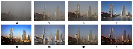
Figure 1.
Example of hazy and dehazed images. The first row contains hazy images of different haze level: (a) heavy haze, (b) moderate haze, (c) slight haze and (d) no haze. The second row contains dehazed images of picture (b) using different dehazing methods: (e) histogram equalization, (f) retinex [23], (g) guided image filter [24] and (h) multi-scale convolutional neural network [25].
In this paper, we propose a series of novel dark and bright channel prior (DBCP)-based methods to fill in the gap in the HLE research for real-world outdoor scenes. The aim of the DBCP methods is not to assess the quality of dehazed images, but to evaluate the haze level in real outdoor scenes. No ground truth image or dehazed image is needed. Only the dark channel and bright channel prior information in a single hazy image is used. Compared with machine learning-based methods, the proposed metrics could be directly and easily calculated without training. An upgraded version of our formerly published real haze image database [26], i.e., RHID_AQI, is adopted as the benchmark dataset. The performances of the DBCP metrics outperform the state-of-the-art blind IQA methods, including haze feature-based and machine learning-based ones.
The rest of the paper is organized as follows. Preliminary knowledge such as physical model, dark channel prior and bright channel prior is presented first in Section 2. The motivation and methodology of the proposed methods are introduced in Section 3. In Section 4, we compare and analyze the performances of different haze IQA algorithms on real haze scene databases. Finally, the conclusion is drawn in Section 5.
2. Background
In this section, we will briefly introduce the atmospheric scattering model as the preliminary knowledge. After that, two successful dehazing models using dark and bright channel prior will be reviewed, respectively.
2.1. Physical Model
In the field of haze removal and haze quality assessment, the following equation is widely used to describe the atmospheric scattering model [27,28]:
where is the observed scene, is the scene radiance at the intersection of the scene with the real-world ray at position , represents the transmission along that ray, and is the global atmospheric light.
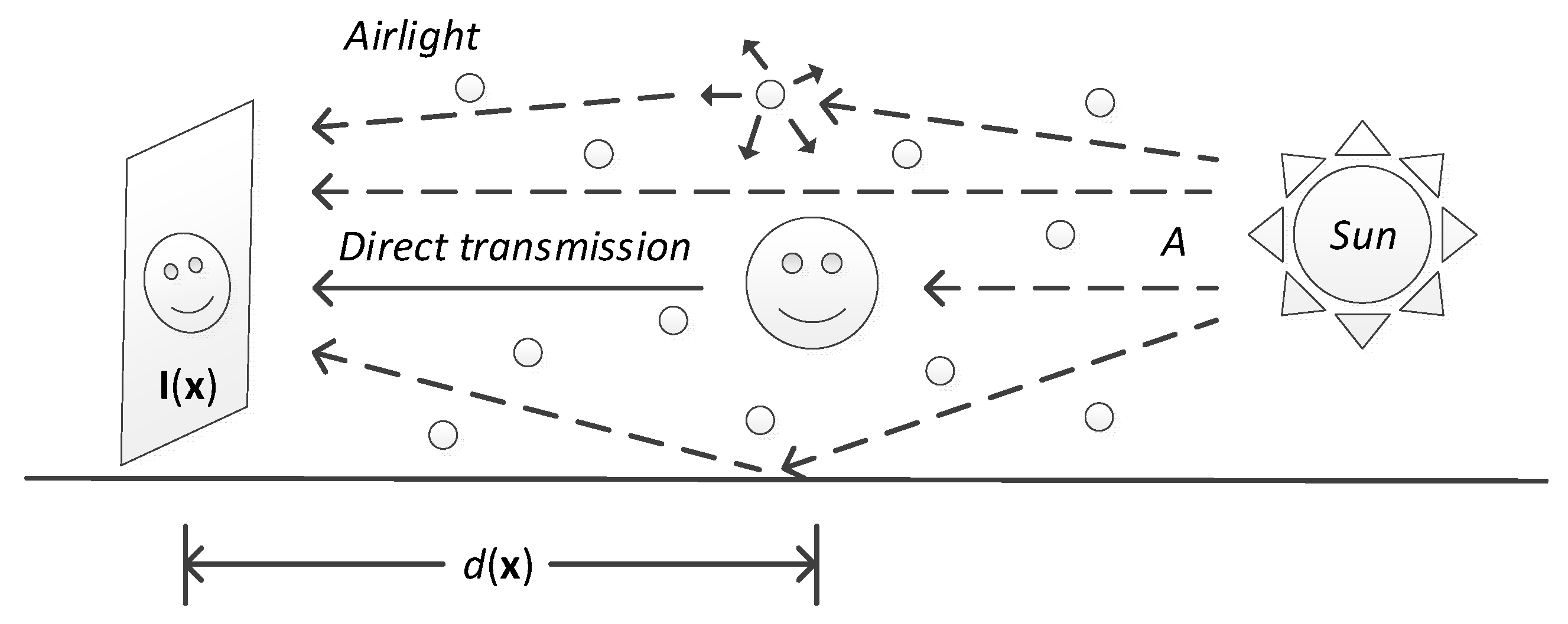
Figure 2 illustrates the model. The formation of an image is decided by two parts: direct transmission and airlight [29,30]. Direct transmission, which corresponds to the first right-side item in (1), represents the attenuation of light received by the camera from the scene point along the line of sight. Airlight, the second item, is the assemble of environmental illumination including sunlight, ground light and skylight reflected into the line of sight by atmospheric particles [31,32].
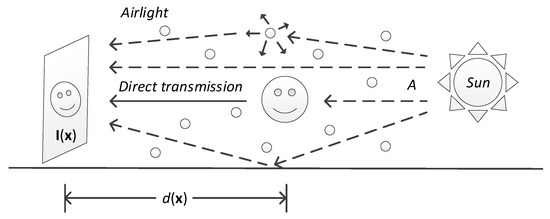
Figure 2.
Illustration of the atmosphere scattering models.
Suppose the atmosphere is homogenous, the transmission is defined as:
where is the scattering coefficient of the atmosphere and is the scene depth. Geometrically, Equation (1) means that in the RGB color space, the vectors , , and are coplanar and their end points are collinear (a detailed description can be found in [27]). Hence the transmission could also be viewed as the ratio of two line segments:
where represents the color channel index.
2.2. Dark Channel Prior
Equation (1) implies the goal of haze removal is to recover , and from . Unfortunately, the problem is inherently ambiguous. He et al. [28] proposed a simple but effective image prior, i.e., dark channel prior, to solve the problem. The dark channel prior (DCP) is a kind of observed statistics for outdoor haze-free images; most local patches contain some pixels whose intensities are very low in at least one color channel. In other words, the minimum value among the red, green and blue channels in such a region is close to zero. The mathematical description of dark channels is as follow:
where is the dark channel of an arbitrary image , is a color channel of , is a local patch centered at , and represents the red, green, and blue color channels, respectively.
According to the DCP theory, the intensity of pixel in an outdoor haze-free image , except for the sky region, is very low and tends to be zero:
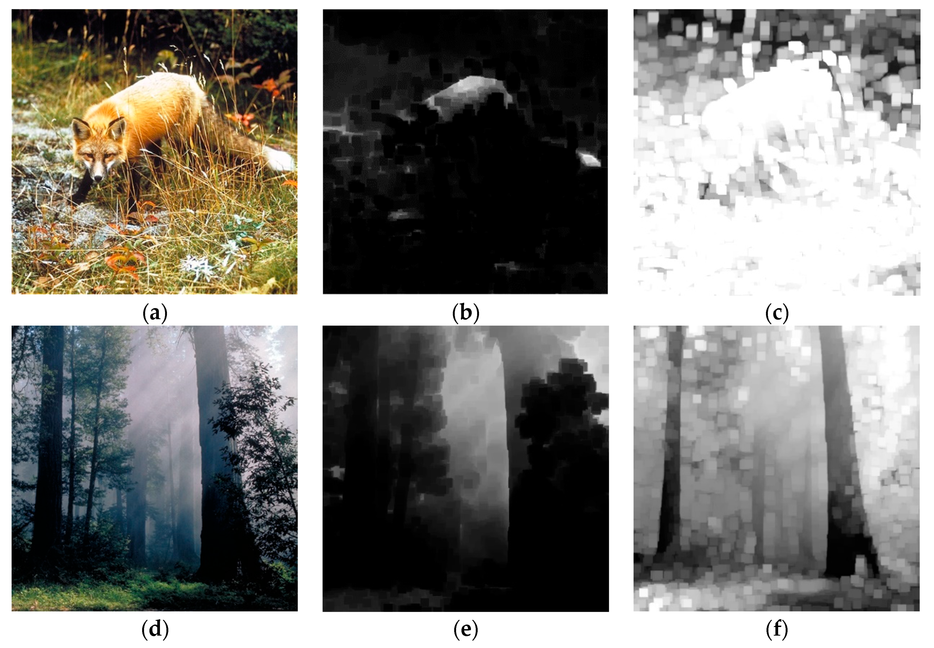
The observation of DCP in real outdoor haze-free and hazy images have been shown in Figure 3. We could see that for the haze-free image, a large number of pixels in the dark channel tend to be zero. While in the dark channel of the hazy picture, the intensities in the middle hazy area remain gray. This difference may contain useful information to reflect the hazy degree in real outdoor scenes, which will be discussed later in Section 3.

Figure 3.
Example images and the corresponding dark and bright channels. (a) is a haze-free example image, (d) is a hazy example image, (b,e) are respectively the corresponding dark channels, and (c,f) are respectively the corresponding bright channels.
2.3. Bright Channel Prior
Inspired by the success of the DCP model, other researchers followed the idea and proposed modified versions, one of which is the bright channel prior (BCP) [33,34]. Like DCP, the BCP focuses on the statistical distribution of image intensities in a local patch and single channel. It is observed that for natural haze-free outdoor images, most local patches include high intensity pixels in at least one color channel, except for some dark regions. Hence, the bright channel is defined as follows:
Suppose the color channel is represented by 8 bits; the highest value in would be 255. The BCP theory could be mathematically expressed as:
Figure 3 demonstrates the observation of BCP in real outdoor scenes. For the haze-free image in the first row, its bright channel is mostly filled with white blocks, as shown in Figure 3c, while in Figure 3f, the hazy regions look gray, and the black trunks remain dark. Like DCP information, BCP differences between hazy and haze-free images might contribute to the HLE problem.
3. Methodology
3.1. Motivation
In previous haze image quality assessment tasks, many researchers used the combination of global atmospheric light, , and transmission, , as the index to reflect the haze degree [33,35]. Although the airlight and transmission could be estimated using dark prior channel information [28], it is still difficult to determine how to construct the combined expression.
From the atmospheric scattering model in Equation (1), we notice that if there is no haze, would be zero and would be equal to . In other words, the change from the “no haze” scene, to the observed “with haze” scene, , is caused by the existence of and . Since it is not easy to design the explicit expression using these two specific parameters, why not change the HLE scheme from bottom-top to top-bottom, i.e., focusing on the overall difference between and ?
Motivated by this inspiration, a series of HLE metrics called DBCP-I, DBCP-II and DBCP-III are proposed in this paper. We will introduce them successively in the following sections.
3.2. DBCP-I
First, we assume that the transmission in a local patch, , is constant and denote it as . For simplicity, we further assume that the atmosphere light, , in the whole scene is constant, and it remains the same in all the channels. We denote this airlight as . Then, we calculate the dark channel on both sides of (1). Equivalently, we put the minimum operators on both sides:
Since is a constant in the patch, it can be moved to the outside of the min operators. Let represent the dark channel on the left side; Equation (8) could be rewritten as:
Since the pixel value in the dark region tends to be zero, could be removed and the estimated transmission calculated by:
For the same local area in a picture, we assume that the transmission, , and airlight, , remain the same. Similarly, by calculating the bright channel on both sides of Equation (1), we have:
where represents the result of .
Substituting (10) into (11), we have:
Thus, the variation between and could be rewritten as:
So far, the dark and bright channel information in an image is calculable, and the air light is estimable [24,28]. This means that the overall difference between and in a bright channel is computable. It is natural to infer that for pictures with different haze levels, the difference between the observed hazy scene, , and the ideal haze-free scene, , will change with the variation of haze level. We believe that in the bright channel, the same rule still applies. Thus, the calculation result in Equation (13) could serve as an indicator of haze level.
Next, we express Equation (13) in a more concise and practical way:
where represents the contrast between and .
As shown in Equation (15), we restrict the bright channel with a lower bound to avoid introducing noise when the bright channel value is 0. A variety of methods for estimating transmission map have been proposed by researchers. In comparison with the roughly estimated transmission map using a dark channel prior [28], the upgraded version that was refined by the guided filter has better structure-transferring properties and faster speed [24]. In this paper we adopt the refined transmission map and denote it as (a detailed definition can be found in Reference [24]). Finally, we average the overall difference by going through the whole image. The proposed haze level evaluation index DBCP-I is defined as:
where and represent the width and height of the image, respectively.
3.3. DBCP-II
Although the DBCP-I already serves as a good HLE index, another label also has satisfactory performance. Particularly, if we view as an image, we found that its segmentation threshold contains useful information to anticipate the haze level. The DBCP-II index is defined as:
where means computing the global image threshold of using Otsu’s method [36]. To better illustrate the DBCP-II method, we compared pictures with same scene but with different haze levels in Figure 4.

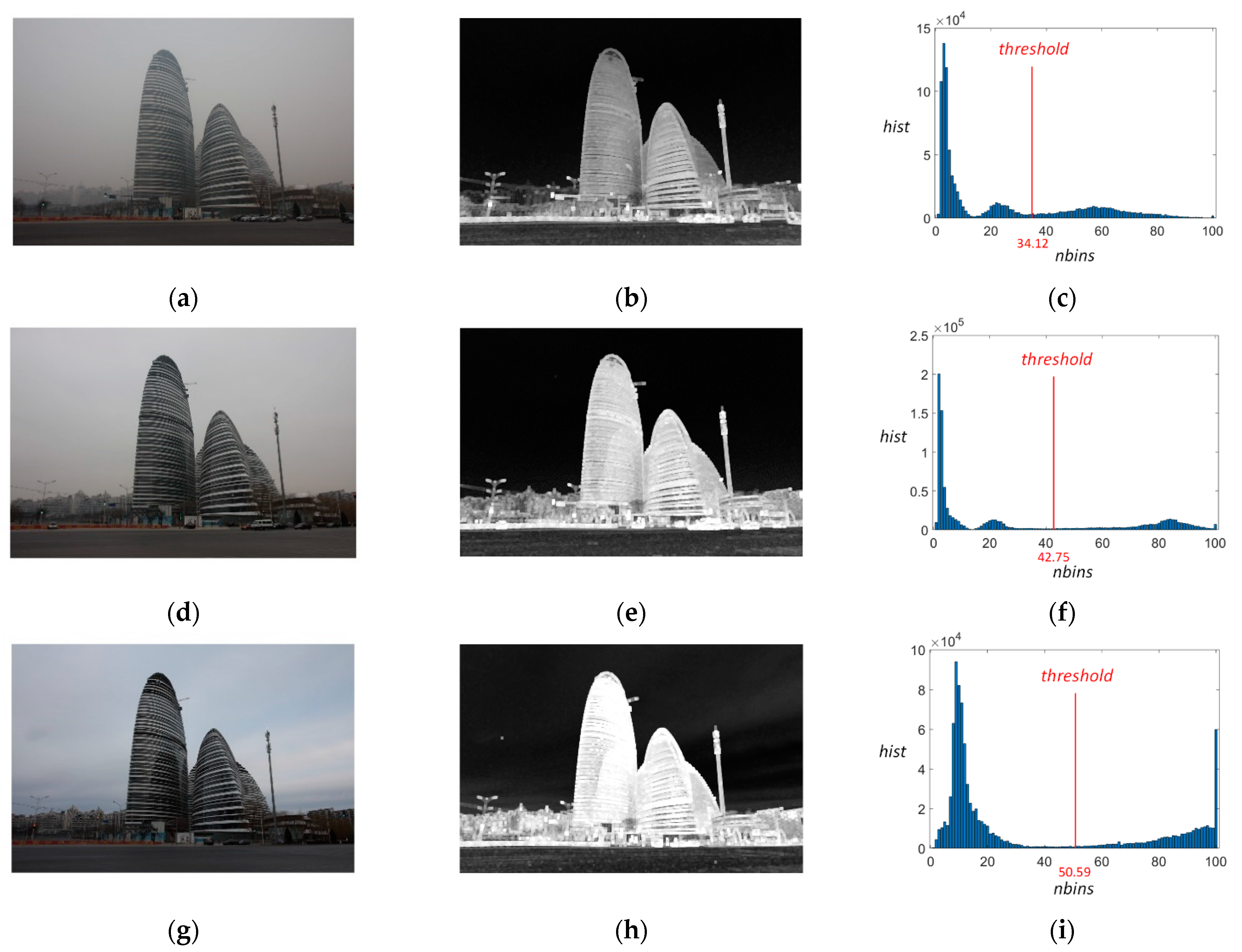
Figure 4.
Illustration of the DBCP-II method. (a,d,g) are examples of heavy, medium and light haze images with same scene. (b,e,h) are the calculated of the corresponding hazy images (a,d,g), respectively; and (c,f,i) are the histograms of (b,e,h), respectively.
According to the definition of , for pixel at a specified position, if its dark channel is equal to its bright channel, the value of would be zero, which means that the dark and bright channels at position have low contrast. On the other side, if is close to zero, we know from the prior information that should be close to 255 and the value of tends to be 1, which implies a high contrast between the dark and bright channels at position . This variation of contrast could be visually observed in Figure 4b,e,h by comparing the background low contrast dark region (tends to be zero) and the foreground high contrast white area (tends to be one). Most importantly, from these figures we notice that the degree of contrast varies with the degree of haziness. For example, in Figure 4b the foreground building looks much darker than that in Figure 4h. In other words, the overall contrast is smaller in the hazy image than in the haze-free image. If we further draw the histogram of and calculate its global threshold for binary segmentation, the threshold values show a good correlation with haze levels, as shown in Figure 4c,f,i.
3.4. DBCP-III
Since both DBCP-I and II work well for HLE problems, it is natural to think of the advantages of combining these two approaches. Let us mine more information from Figure 4. As mentioned above, the calculated segmentation threshold divides into two parts: low contrast area and high contrast area . Take the first row (heavy haze) in Figure 4 as an example; indicates the sky and the gray road in Figure 4a, the black and dark gray area in Figure 4b, and the neighborhood of the two highest peaks in Figure 4c. For pixels in , DBCP-II is a better choice because both the numerator and the denominator in Formula (14) tend to be very small, which would introduce more noise and uncertainty to the result of division. Meanwhile for the remaining pixels in , representing scene details and contents, DBCP-I is a better choice for accurately calculating the changes between dark and bright channels. In brief, the combined index is constructed as follow:
where represents the estimated HLE index in position , and the calculation of DBCP-III is defined as:
4. Experimental Results and Discussion
4.1. Evaluation Index
In an IQA field, the Pearson correlation coefficient (PCC) is usually used to measure the prediction linearity, and the Spearman rank order correlation coefficient (SROCC) is adopted to evaluate the prediction monotonicity. For HLE problem, we use the same evaluation indexes. The definitions of PCC and SROCC are as follows:
where is the total number of images in the database; and denote the i-th subjective and objective scores, respectively; and represent the mean value of the subjective and objective quality scores in each image set, respectively; and is the i-th difference between the ranks in the two image sets.
Additionally, the normally existed nonlinearity between predicted image quality scores and subjective grades needs to be eliminated before we calculate the evaluation index. Specifically, a five-parameter nonlinear logistic regression is recommended by the video quality expert group [37]:
where represents the mapped objective score, denotes the predicted quality score, and through are the model fitting parameters.
4.2. Datasets
With the rapid development of haze model and dehazing methods evaluation techniques, a variety of hazy image databases have appeared. Among them some are designed for HLE problems [26,35,38,39], while the others are designed to provide a benchmark for dehazing algorithms [14,16,17,18,19,20,21,22,40,41,42]. Figure 5 shows some hazy images in these databases.
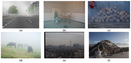
Figure 5.
Example hazy images in typical datasets: (a) IBHLED [39], (b) CHIC [16], (c) O-HAZE [41], (d) DHQ [19], (e) exBeDDE [22] and (f) RHID_AQI [26].
The hazy datasets could be further categorized. For example, Figure 5a shows a hazy image in the image-based haze level estimation dataset (IBHLED) [39], which contains 3024 synthetic images and their haze level labels. In the IBHLED database, both the ground truths and hazy images are generated by computer. To better simulate real scene dehazing scenarios, researchers adopted real indoor and outdoor haze-free images and generated hazy pictures using professional haze machines, as shown in Figure 5b,c, respectively. Figure 5d represents the most typical real hazy image in recently published dehazing databases like DHQ [19], RESIDE [17], SHRQ [20], NH-HAZE [21] and BeDDE [22]. In these datasets a hazy image is usually adopted as ground truth to generate dehazing counterparts, and the subjective scores (if available) usually belong to the dehazed ones. One exception comes from the extension version of BeDDE, i.e., exBeDDE [22], where the authors provided natural outdoor scenes together with intra-class subjective scores. Figure 5e shows a hazy scene captured in Hong Kong in the exBeDDE dataset. In the picture, the black edge was seen because images in the same group were spatially calibrated. The last introduced database comes from the real haze image database with a air quality information (RHID_AQI) dataset. It is an upgraded version of our formerly published dataset, i.e., HID2016 [26]. The aim of RHID_AQI is to evaluate the quality of outdoor hazy images. A total of 301 outdoor natural images taken in 8 different cities are provided, with subjective scores of compliance with the ITU-R_BT.500-11 protocol [43]. In this paper we use the RHID_AQI and exBeDDE datasets as simulation benchmarks because only they offer ground truth subjective scores for real haze images.
4.3. Performance Comparison
4.3.1. Implementation Details
Three groups of no-reference (NR) IQA metrics are compared with the proposed DBCP metrics. The first group comprises haze level-related features extracted from haze images directly, such as [35], [39], [33], [44], [45], [45], [45] and [46]. The second group is made up of pre-trained machine learning algorithms designed for rich types of scenes like natural pictures, screen content images, contrast-distorted images, etc. Specifically, the IQA models include: QAC [47], NIQE [48], LPSI [49], IL-NIQE [50], HOSA [51], dipIQ [52], UCA [53], NIQMC [54], BPRI(p) [55], BPRI(c) [55], BMPRI [56], BIQME [57] and MEON [58]. The third group consists of two deep neural networks for general-purpose NR IQA tasks: CNN [59] and DIQaM-NR [60]. Similar to Reference [61], we randomly divided the dataset into two parts: 80% for training and 20% for testing. This process was repeated ten times and the results were averaged. Finally, for the DBCP metrics, the window size was set to 9 × 9 for both dark channel and bright channel computation.
4.3.2. Experiment Results on RHID_AQI
To the best of our knowledge, the RHID_AQI database is the only one designed for haze level evaluation tasks with highly credible subjective ratings. We use it to serve as the benchmark dataset. The SROCC and PCC values of the IQA models mentioned in Section 4.3.1 are listed in Table 1.

Table 1.
Comparison of SROCC and PCC on the RHID_AQI database.
In each column of Table 1, the three best-performing models are highlighted in bold. From the ranking we could see that the DBCP-II metric performs best when considering both the SROCC and PCC evaluation indexes. We also found that for all the hazy images in the dataset, the best-performing algorithms are concentrated in the DBCP group and deep neural network group. Compared with these two groups, the image feature group and machine learning group perform poorly.
To further observe the individual scene performance, the SROCC values of different NR IQA metrics are compared in Table 2. Similarly, we show the top three scores for each city in bold and the number of hits for each model. The comparison results further validate the advantages of the DBCP family, especially for the hybrid method DBCP-III. The SROCC scores of DBCP-III are among top 3 for 7 out of 8 cities.
Table 2.
Comparison of SROCC on individual scenes in the RHID_AQI database.
Meanwhile, the performances of the pre-trained machine learning family are still at the bottom. This makes sense from two perspectives. First, the algorithms in the machine learning group mainly focus on image destruction or image degradation, not on haze level evaluation. Second, the type of the pre-trained datasets are images with natural scenes or screen content, which are quite different from real-world hazy images.
4.3.3. Experiment Results on exBeDDE
Although the proposed DBCP metrics have proven their effectiveness and superiority in the RHID_AQI database, we would like to check their generalization ability on other datasets. To the best of our knowledge, the RHID_AQI and exBeDDE databases are the only two datasets whose image pairs were collected in natural outdoor scenes without any simulation and who offer subjective scores. Table 3 shows the SROCC experiment results on the exBeDDE dataset. Note that the scores offered by the exBeDDE were defined in groups and should never be used between groups [22]; We only compared the evaluation index of the twelve individual cities but not of the whole dataset. To better observe the stability of the IQA models in different scenes, we calculated the mean value of the SROCC values along all the individual cities for each model. Meanwhile, when calculating the DBCP scores, a margin with a width of 128 pixels was cut off from the hazy images to eliminate the influence of image alignment in the construction of the exBeDDE dataset.
Table 3.
Comparison of SROCC on individual scenes in the exBeDDE database.
Overall, the comparison results in Table 3 are satisfactory. Same as before, the top 3 winners are highlighted in bold and the number of hits for each method is counted. The proposed DBCP-III metric once again wins first place in terms of hit count, and the no-reference machine learning group still falls behind. The deep learning group showed significant regression in some individual scenes. The reason might be the small sample size for these cities, which is a common problem for training-based IQA approaches.
4.4. Performance Analysis
Based on the design of the DBCP-III, it is supposed to have better performance. It is true for most cases when comparing the results in Table 1, Table 2 and Table 3. However, for the overall situation in the RHID_AQI dataset as well as several individual cities, the performances of the hybrid method are not the best. Meanwhile, the performance level only falls a little in comparison with the winners of the other two candidates in the DBCP family.
Obviously, the DBCP-I and DBCP-II methods have their own scenarios that are more applicable, and both of the approaches have their drawbacks. The first metric is not suitable for areas with low transmittance and the inclusion of that region will introduce noise. This is why, in most cases, DBCP-I performs worse than the other two. Conversely, for Lasa in the RHID_AQI dataset, DBCP-I won the first place because the pictures captured in this city have less haze and high transmittance [26].
As for the second one, the segmentation accuracy is a key factor. If the ratio of high contrast pixels to low contrast pixels in is mismatched, the accuracy of the segmentation threshold will be affected. According to the definition, the value of will move to zero when the pixels in dark and bright channels are similar. Although this is a good property for examining the degree of haze, it may be affected by the gray region. This type of area has exactly same dark and bright channels, and it will introduce a large number of zeros to . Therefore, for scenes with large gray areas, both the results of DBCP-I and DBCP-II might be affected, and this explains why for Taiyuan in the RHID_AQI database, the performances of these two metrics are unsatisfactory.
Fortunately, the deficiencies of DBCP-I and DBCP-II can be remedied by DBCP-III, which has been explained in Section 3.4. Most of the experimental data have proven the effectiveness, especially for Taiyuan, and it should be admitted that for cases that DBCP-I or DBCP-II perform extremely well, the introduction of the hybrid method might neutralize part of the original outstanding performance. Overall, the performance of DBCP-III is better or at least comparable to the other two.
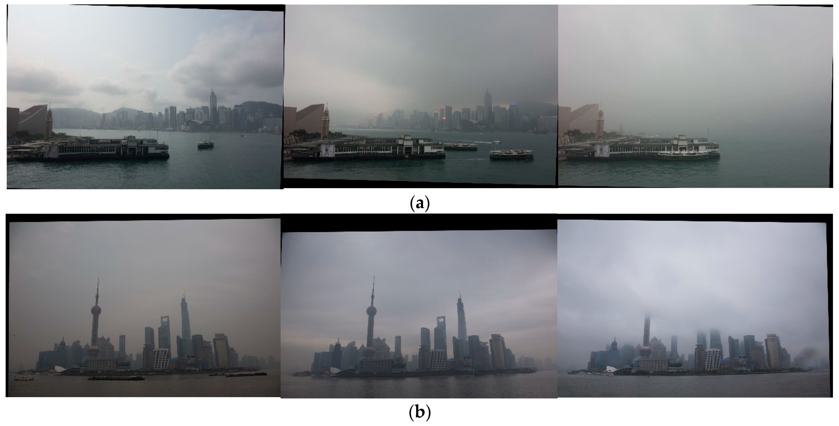
In the exBeDDE dataset, there are two scenes worth noting. The DBCP-based methods are not good for Hongkong and Shanghai. The reasons may be two-fold. On one hand, the numbers of hazy images of these two cities are too small. There are only 13 pictures for Hongkong and 8 images for Shanghai. On the other hand, the content in these two scenes varies considerably, as shown in Figure 6. The variance of the boats in the first row and the disappearance of the top of the building in the second row might introduce uncertainty into the evaluation results.
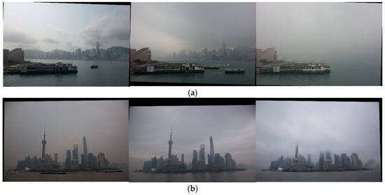
Figure 6.
Example hazy images in the exBeDDE dataset: (a) Hongkong and (b) Shanghai.
4.5. Effect of Window Size
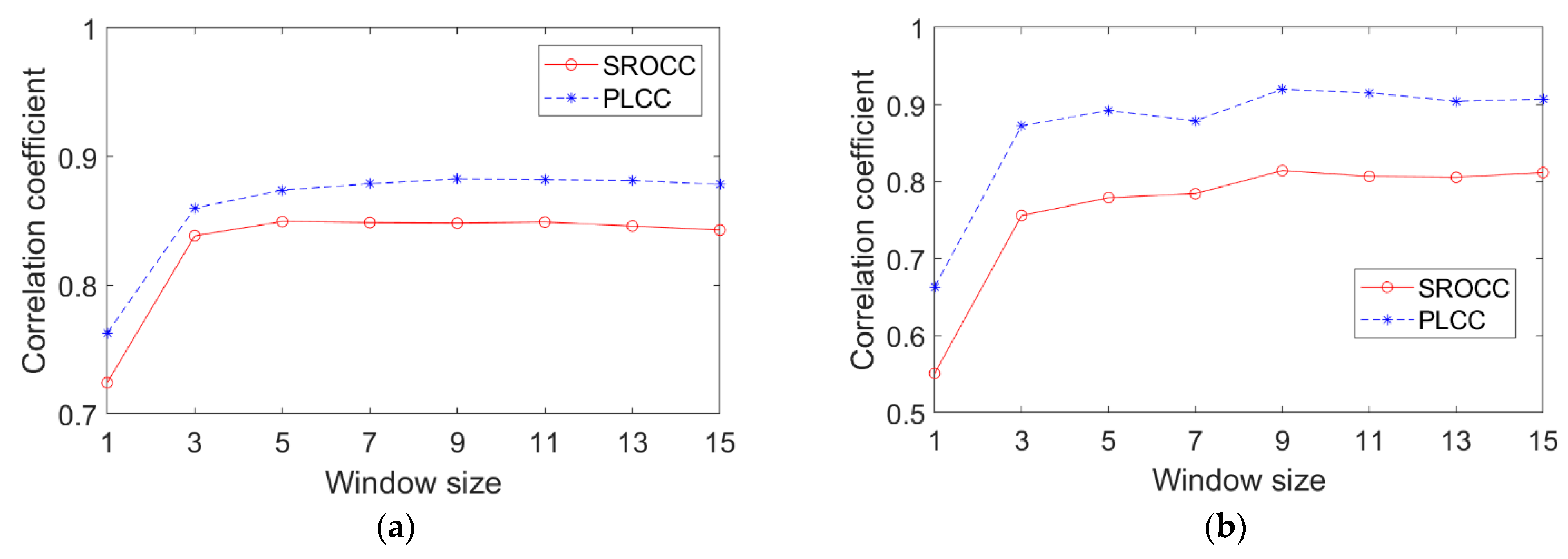
As described, the only parameter that needs to be set in the DBCP algorithms is the size of the template window when calculating the dark and bright channels. Here we selected different window sizes from 1 × 1 to 15 × 15 to observe the influence of this parameter in Figure 7. Take the DBCP-III metric for example; for each size, the averaged SROCC and PLCC values along overall and individual cities on the RHID_AQI database are calculated and indicated in Figure 7a, and the mean values along single cities in the exBeDDE dataset are illustrated in Figure 7b. The simulation results show that the performance of the algorithm is not sensitive to the variation of window size except for the situation of 1 × 1. In this case the template window is no longer an actual window but a pixel, and it is easy to anticipate the performance degradation. Based on the whole performance for various DBCP metrics on the two datasets, also considering the computation cost, we choose a window size of 9 × 9 for recommendation.
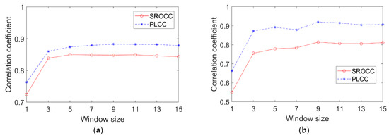
Figure 7.
Comparison of the average SROCC and PLCC values with respect to different window sizes for the DBCP-III method on the (a) RHID_AQI dataset and (b) exBeDDE dataset.
4.6. Computation Cost
As introduced, one of the purposes of HLE algorithms is to provide not only accurate but also fast index for the advanced driver assistance system. Hence, the computation cost of each algorithm is an important factor. Based on the performances of the methods in Section 4.3, we chose some relatively outstanding candidates to compare their computation speeds. The configuration of our CPU computer is an Intel(R) Core (TM) i7-4790 CPU at 3.60 GHz with 12 GB RAM, and the GPU model is GTX1080ti with 11 GB RAM. The comparison results of average computing time per image in the RHID_AQI dataset are shown in Table 4.
Table 4.
Comparison of computation cost on the RHID_AQI database.
From the table, we notice that the model of C is the fastest one. However, its HLE performance is not comparable to the other candidates. The deep learning group is fast too, but the configuration of the GUP computer is much higher than that of the CUP computer. The DBCP-II algorithm is faster than D, which is the best performer in the haze level-related feature group. As for the DBCP-I and DBCP-III metrics, although they are not as fast as the other competitors, the difference is not huge. In addition, the proposed DBCP metrics require no training time compared to the machine learning or deep learning groups, which is a potential advantage for time saving.
5. Conclusions
In this paper, we propose a series of simple but efficient DBCP metrics to evaluate the degree of haziness in real outdoor scenes. The presented methods utilize dark and bright channel prior information in a single image. The calculation process needs no training or learning, and only one parameter, i.e., window size, is required to be set. The algorithms not only have superior performances, but also have competitive computational speed. These features increase the practicability of the proposed methods. Furthermore, the study fills the gap in the field of haze level evaluation.
Of course, the proposed methods have their drawbacks. For DBCP-I, since it is inspired by the dark and bright channel prior, similar limitations for areas like sky, shadow, gray and white regions still exist [28,33]. Fortunately, in DBCP-II we discover an adaptive threshold and in DBCP-III we eliminate the influence of these regions by introducing the piecewise function. In addition, the potential auto-driving application scenario requires a high speed of evaluation. Hence improving the evaluation speed and transferring the idea from picture to video will be our future research focus.
Author Contributions
Conceptualization, Y.C.; methodology, Y.C.; validation, Y.C. and F.C.; formal analysis, Y.C.; writing—original draft preparation, Y.C.; writing—review and editing, H.F. and H.Y.; funding acquisition, Y.C. All authors have read and agreed to the published version of the manuscript.
Funding
This research was funded by the Stabilization Support Plan for Shenzhen Higher Education Institutions, grant number 20200812165210001.
Data Availability Statement
The source codes and the benchmark dataset, i.e., RHID_AQI, are free to download from the following websites: https://drive.google.com/file/d/1k27q8aFLdXbLXThrfcgv2TLCtMmujnwU/view?usp=sharing, or https://pan.baidu.com/s/18tGocrcd2RsO8kUPj2ecKA with password DBCP (accessed on 20 April 2022).
Acknowledgments
We thank the siyuefeng.com (accessed on 22 March 2022) website who held the public benefit photographic exhibition, i.e., “The breath of China” in 2014, and thank the organizer and the photographers who authorized us to use the photos to build the RHID_AQI database. Specifically, we want to thank the following photographers who took the haze pictures, including: Yingjiu Zhao and Duona Fu in Beijing, Jianshi Zhou in Hangzhou, Hong Shu and Qing Xia in Kunming, Hao Luo and Dui Zha in Lasa, Xiaojun Guo and Bing Hu in Shijiazhuang, Jiang Liu in Taiyuan, Ye Xue and Xinjie Wu in Tianjin, and Xiaojuan Pan in Wuhan.
Conflicts of Interest
The authors declare no conflict of interest. The funders had no role in the design of the study; in the collection, analyses, or interpretation of data; in the writing of the manuscript, or in the decision to publish the results.
References
- Wang, Z.; Bovik, A.C.; Sheikh, H.R.; Simoncelli, E.P. Image quality assessment: From error visibility to structural similarity. IEEE Trans. Image Process. 2004, 13, 600–612. [Google Scholar] [CrossRef] [PubMed] [Green Version]
- Chen, G.-H.; Yang, C.-L.; Po, L.-M.; Xie, S.-L. Edge-based structural similarity for image quality assessment. In Proceedings of the 2006 IEEE International Conference on Acoustics Speed and Signal Processing Proceedings, Toulouse, France, 14–19 May 2006; Volume 2, p. 2. [Google Scholar] [CrossRef] [Green Version]
- Chen, G.-H.; Yang, C.-L.; Xie, S.-L. Gradient-based structural similarity for image quality assessment. In Proceedings of the 2006 International Conference on Image Processing, Atlanta, GA, USA, 8–11 October 2006; pp. 2929–2932. [Google Scholar] [CrossRef]
- Zhang, L.; Zhang, L.; Mou, X. RFSIM: A feature based image quality assessment metric using Riesz transforms. In Proceedings of the 2010 IEEE International Conference on Image Processing, Hong Kong, China, 26–29 September 2010; pp. 321–324. [Google Scholar] [CrossRef] [Green Version]
- Zhang, L.; Zhang, L.; Mou, X.; Zhang, D. FSIM: A feature similarity index for image quality assessment. IEEE Trans. Image Process. 2011, 20, 2378–2386. [Google Scholar] [CrossRef] [Green Version]
- Wang, Z.; Sheikh, H.; Bovik, A. No-reference perceptual quality assessment of JPEG compressed images. In Proceedings of the International Conference on Image Processing, Rochester, NY, USA, 22–25 September 2002; Volume 1, pp. I-477–I-480. [Google Scholar] [CrossRef] [Green Version]
- Wang, Z.; Simoncelli, E.P.; Bovik, A.C. Multiscale structural similarity for image quality assessment. In Proceedings of the Thrity-Seventh Asilomar Conference on Signals, Systems & Computers, Pacific Grove, CA, USA, 9–12 November 2003; Volume 2, pp. 1398–1402. [Google Scholar] [CrossRef] [Green Version]
- Shen, J.; Li, Q.; Erlebacher, G. Hybrid no-reference natural image quality assessment of noisy, blurry, JPEG2000, and JPEG images. IEEE Trans. Image Process. 2011, 20, 2089–2098. [Google Scholar] [CrossRef] [PubMed]
- Xue, W.; Mou, X.; Zhang, L.; Bovik, A.; Feng, X. Blind image quality assessment using joint statistics of gradient magnitude and laplacian features. IEEE Trans. Image Process. 2014, 23, 4850–4862. [Google Scholar] [CrossRef] [PubMed]
- Simoncelli, E.P. Statistical models for images: Compression, restoration and synthesis. In Proceedings of the Conference Record of the Thirty-First Asilomar Conference on Signals, Systems and Computers (Cat. No.97CB36136), Pacific Grove, CA, USA, 2–5 November 1997; pp. 673–678. [Google Scholar] [CrossRef]
- Simoncelli, E.P. Modeling the joint statistics of images in the wavelet domain. In Proceedings of the International Society for Optical Engineering, Denver, CO, USA, 19–23 July 1999; Volume 3813, pp. 188–195. [Google Scholar] [CrossRef]
- Simoncelli, E.P.; Schwartz, O. Modeling surround suppression in V1 neurons with a statistically-derived normalization model. Adv. Neural Inf. Process. Syst. 1999, 11, 153–159. [Google Scholar]
- Wainwright, M.J.; Simoncelli, E.P. Scale mixtures of gaussians and the statistics of natural images. Adv. Neural Inf. Process. Syst. 2000, 12, 855–861. [Google Scholar]
- Ma, K.; Liu, W.; Wang, Z. Perceptual evaluation of single image dehazing algorithms. In Proceedings of the 2015 IEEE International Conference on Image Processing, Quebec City, QC, Canada, 27–30 September 2015. [Google Scholar]
- Ancuti, C.; Codruta, A.; Vleeschouwer, C. D-HAZY: A dataset to evaluate quantitatively dehazing algorithms. In Proceedings of the 2016 IEEE International Conference on Image Processing, Phoenix, AZ, USA, 25–28 September 2016. [Google Scholar]
- Mansouri, A.; Nouboud, F.; Chalifour, A.; Mammass, D.; Meunier, J.; Elmoataz, A. A color image database for haze model anddehazing methods evaluation. In Proceedings of the International Conference on Image and Signal Processing, Trois-Rivieres, QC, Canada, 30 May–1 June 2016; Springer: Berlin/Heidelberg, Germany, 2016. Chapter 12. pp. 109–117. [Google Scholar]
- Li, B.; Ren, W.; Fu, D.; Tao, D.; Feng, D.; Zeng, W.; Wang, Z. Benchmarking single-image dehazing and beyond. IEEE Trans. Image Process. 2018, 28, 492–505. [Google Scholar] [CrossRef] [Green Version]
- Zhang, Y.; Ding, L.; Sharma, G. HazeRD: An outdoor scene dataset and benchmark for single image dehazing. In Proceedings of the 2017 IEEE International Conference on Image Processing, Beijing, China, 17–20 September 2017. [Google Scholar]
- Min, X.; Zhai, G.; Gu, K.; Yang, X.; Guan, X. Objective quality evaluation of dehazed images. IEEE Trans. Intell. Transp. Syst. 2018, 20, 2879–2892. [Google Scholar] [CrossRef]
- Min, X.; Zhai, G.; Gu, K.; Zhu, Y.; Zhou, J.; Guo, G.; Yang, X.; Guan, X.; Zhang, W. Quality evaluation of image dehazing methods using synthetic hazy images. IEEE Trans. Multimed. 2019, 21, 2319–2333. [Google Scholar] [CrossRef]
- Ancuti, C.O.; Ancuti, C.; Timofte, R. NH-HAZE: An image dehazing benchmark with non-homogeneous hazy and haze-free images. In Proceedings of the 2020 IEEE/CVF Conference on Computer Vision and Pattern Recognition Workshops, Seattle, WA, USA, 14–19 June 2020. [Google Scholar]
- Zhao, S.; Zhang, L.; Huang, S.; Shen, Y.; Zhao, S. Dehazing evaluation: Real-world benchmark datasets, criteria, and baselines. IEEE Trans. Image Process. 2020, 29, 6947–6962. [Google Scholar] [CrossRef]
- Land, E.H. The Retinex. In Ciba Foundation Symposium-Colour Vision: Physiology and Experimental Psychology; Wiley: Hoboken, NJ, USA, 1965; pp. 217–227. [Google Scholar]
- He, K.; Sun, J.; Tang, X. Guided image filtering. IEEE Trans. Pattern Anal. Mach. Intell. 2013, 35, 1397–1409. [Google Scholar] [CrossRef] [PubMed]
- Ren, W.; Liu, S.; Zhang, H.; Pan, J.; Cao, X.; Yang, M.H. Single image dehazing via multi-scale convolutional neural networks. In Proceedings of the 14th European Conference on Computer Vision, Amsterdam, The Netherlands, 8–16 October 2016. [Google Scholar]
- Chu, Y.; Chen, Z.; Fu, Y.; Yu, H. Haze image database and preliminary assessments. In Proceedings of the Fully3D Conference, Xi’an, China, 18–23 June 2017; pp. 825–830. [Google Scholar]
- Fattal, R. Single image dehazing. ACM Trans. Graph. 2008, 27, 1–9. [Google Scholar] [CrossRef]
- He, K.; Sun, J.; Tang, X. Single image haze removal using dark channel prior. IEEE Trans. Pattern Anal. Mach. Intell. 2011, 33, 2341–2353. [Google Scholar] [CrossRef] [PubMed]
- Narasimhan, S.; Nayar, S. Chromatic framework for vision in bad weather. In Proceedings of the IEEE Conference on Computer Vision and Pattern Recognition, Hilton Head, SC, USA, 15 June 2000; Volume 1, pp. 598–605. [Google Scholar]
- Narasimhan, S.G.; Nayar, S.K. Vision and the atmosphere. Int. J. Comput. Vis. 2002, 48, 233–254. [Google Scholar] [CrossRef]
- Narasimhan, S.G.; Nayar, S.K. Contrast restoration of weather degraded images. IEEE Trans. Pattern Anal. Mach. Intell. 2003, 25, 713–724. [Google Scholar] [CrossRef] [Green Version]
- Tan, R.T. Visibility in bad weather from a single image. In Proceedings of the 2008 IEEE Conference on Computer Vision and Pattern Recognition, Anchorage, AK, USA, 23–28 June 2008; pp. 1–8. [Google Scholar] [CrossRef]
- Fu, X.; Lin, Q.; Guo, W.; Ding, X.; Huang, Y. Single image de-haze under non-uniform illumination using bright channel prior. J. Theor. Appl. Inf. Technol. 2013, 48, 1843–1848. [Google Scholar]
- Wang, Y.T.; Zhuo, S.J.; Tao, D.P.; Bu, J.J.; Li, N. Automatic local exposure correction using bright channel prior for under-exposed images. Signal Process. 2013, 93, 3227–3238. [Google Scholar] [CrossRef]
- Zhan, Y.; Zhang, R.; Wu, Q.; Wu, Y. A new haze image database with detailed air quality information and a novel no-reference image quality assessment method for haze images. In Proceedings of the 2016 IEEE International Conference on Acoustics, Speech and Signal Processing (ICASSP), Shanghai, China, 20–25 March 2016; Springer: Berlin/Heidelberg, Germany, 2016; pp. 1095–1099. [Google Scholar]
- Otsu, N. A threshold selection method from gray-level histograms. IEEE Trans. Syst. Man Cybern. 1979, 9, 62–66. [Google Scholar] [CrossRef] [Green Version]
- VQEG. Final Report from the Video Quality Experts Group on the Validation of Objective Models of Video Quality Assessment—Phase II. 2003. Available online: http://www.vqeg.org (accessed on 20 April 2022).
- Tarel, J.-P.; Hautiere, N.; Caraffa, L.; Cord, A.; Halmaoui, H.; Gruyer, D. Vision enhancement in homogeneous and heterogeneous fog. IEEE Intell. Transp. Syst. Mag. 2012, 4, 6–20. [Google Scholar] [CrossRef] [Green Version]
- Li, Y.; Huang, J.; Luo, J. Using user generated online photos to estimate and monitor air pollution in major cities. In Proceedings of the 7th International Conference on Internet Multimedia Computing and Service, Zhangjiajie, China, 19 August 2015; pp. 11–15. [Google Scholar] [CrossRef] [Green Version]
- Ancuti, C.; Ancuti, C.O.; Timofte, R.; De Vleeschouwer, C. I-HAZE: A dehazing benchmark with real hazy and haze-free indoor images. In Proceedings of the 19th International Conference on Advanced Concepts for Intelligent Vision Systems, Poitiers, France, 24–27 September 2018; Volume 11182, pp. 620–631. [Google Scholar] [CrossRef] [Green Version]
- Ancuti, C.O.; Ancuti, C.; Timofte, R.; De Vleeschouwer, C. O-HAZE: A dehazing benchmark with real hazy and haze-free outdoor images. In Proceedings of the 31st Meeting of the IEEE/CVF Conference on Computer Vision and Pattern Recognition Workshops, Salt Lake City, UT, USA, 18–22 June 2018; pp. 867–875. [Google Scholar] [CrossRef] [Green Version]
- Ancuti, C.O.; Ancuti, C.; Sbert, M.; Timofte, R. Dense-haze: A benchmark for image dehazing with dense-haze and haze-free images. In Proceedings of the 26th IEEE International Conference on Image Processing, Taipei, Taiwan, 22–25 September 2019; pp. 1014–1018. [Google Scholar] [CrossRef] [Green Version]
- ITU-T, Geneva, Switzerland: Methodology for the Subjective Assessment of the Quality of Television Pictures. Recommendation ITU-R BT.500-11. Available online: https://www.itu.int/rec/R-REC-BT.500 (accessed on 20 April 2022).
- CHsieh, C.-H.; Horng, S.-C.; Huang, Z.-J.; Zhao, Q. Objective haze removal assessment based on two-objective optimization. In Proceedings of the 2017 IEEE 8th International Conference on Awareness Science and Technology, Taichung, Taiwan, 8–10 November 2017; pp. 279–283. [Google Scholar] [CrossRef]
- Lu, H.; Zhao, Y.; Zhao, Y.; Wen, S.; Ma, J.; Keung, L.H.; Wang, H. Image defogging based on combination of image bright and dark channels. Guangxue Xuebao (Acta Opt. Sin.) 2018, 38, 1115004. [Google Scholar] [CrossRef]
- Choi, L.K.; You, J.; Bovik, A. Referenceless prediction of perceptual fog density and perceptual image defogging. IEEE Trans. Image Process. 2015, 24, 3888–3901. [Google Scholar] [CrossRef] [PubMed]
- Xue, W.; Zhang, L.; Mou, X. Learning without human scores for blind image quality assessment. In Proceedings of the 2013 IEEE Conference on Computer Vision and Pattern Recognition, Portland, OR, USA, 23–28 June 2013; pp. 995–1002. [Google Scholar] [CrossRef] [Green Version]
- Mittal, A.; Soundararajan, R.; Bovik, A. Making a ‘completely blind’ image quality analyzer. IEEE Signal Process. Lett. 2013, 20, 209–212. [Google Scholar] [CrossRef]
- Wu, Q.; Wang, Z.; Li, H. A highly efficient method for blind image quality assessment. In Proceedings of the 2015 IEEE International Conference on Image Processing, Quebec City, QC, Canada, 27–30 September 2015; pp. 339–343. [Google Scholar] [CrossRef]
- Zhang, L.; Zhang, L.; Bovik, A. A feature-enriched completely blind image quality evaluator. IEEE Trans. Image Process. 2015, 24, 2579–2591. [Google Scholar] [CrossRef] [PubMed] [Green Version]
- Xu, J.; Ye, P.; Li, Q.; Du, H.; Liu, Y.; Doermann, D.S. Blind image quality assessment based on high order statistics aggregation. IEEE Trans. Image Process. 2016, 25, 4444–4457. [Google Scholar] [CrossRef] [PubMed]
- Ma, K.; Liu, W.; Liu, T.; Wang, Z.; Tao, D. dipIQ: Blind image quality assessment by learning-to-rank discriminable image pairs. IEEE Trans. Image Process. 2017, 26, 3951–3964. [Google Scholar] [CrossRef] [PubMed] [Green Version]
- Min, X.; Ma, K.; Guangtao, Z.; Zhai, G.; Wang, Z.; Lin, W. Unified blind quality assessment of compressed natural, graphic, and screen content images. IEEE Trans. Image Process. 2017, 26, 5462–5474. [Google Scholar] [CrossRef]
- Gu, K.; Lin, W.; Zhai, G.; Yang, X.; Zhang, W.; Chen, C.W. No-reference quality metric of contrast-distorted images based on information maximization. IEEE Trans. Cybern. 2017, 47, 4559–4565. [Google Scholar] [CrossRef]
- Min, X.; Gu, K.; Zhai, G.; Liu, J.; Yang, X.; Chen, C.W. Blind quality assessment based on pseudo-reference image. IEEE Trans. Multimed. 2018, 20, 2049–2062. [Google Scholar] [CrossRef]
- Min, X.; Zhai, G.; Gu, K.; Liu, Y.; Yang, X. Blind image quality estimation via distortion aggravation. IEEE Trans. Broadcast. 2018, 64, 508–517. [Google Scholar] [CrossRef]
- Gu, K.; Tao, D.; Qiao, J.-F.; Lin, W. Learning a no-reference quality assessment model of enhanced images with big data. IEEE Trans. Neural Netw. Learn. Syst. 2018, 29, 1301–1313. [Google Scholar] [CrossRef] [Green Version]
- Ma, K.; Liu, W.; Zhang, K.; Duanmu, Z.; Wangmeng, Z.; Zuo, W. End-to-end blind image quality assessment using deep neural networks. IEEE Trans. Image Process. 2017, 27, 1202–1213. [Google Scholar] [CrossRef] [PubMed]
- Kang, L.; Ye, P.; Li, Y.; Doermann, D. Convolutional neural networks for no-reference image quality assessment. In Proceedings of the 2014 IEEE Computer Vision and Pattern Recognition, Columbus, OH, USA, 23–28 June 2014; pp. 1733–1740. [Google Scholar] [CrossRef] [Green Version]
- Bosse, S.; Maniry, D.; Muller, K.-R.; Wiegand, T.; Samek, W. Deep neural networks for no-reference and full-reference image quality assessment. IEEE Trans. Image Process. 2017, 27, 206–219. [Google Scholar] [CrossRef] [PubMed] [Green Version]
- Liu, X.; Van De Weijer, J.; Bagdanov, A.D. RankIQA: Learning from rankings for no-reference image quality assessment. In Proceedings of the 2017 IEEE International Conference on Computer Vision, Venice, Italy, 22–29 October 2017; pp. 1040–1049. [Google Scholar] [CrossRef] [Green Version]


Publisher’s Note: MDPI stays neutral with regard to jurisdictional claims in published maps and institutional affiliations. |
© 2022 by the authors. Licensee MDPI, Basel, Switzerland. This article is an open access article distributed under the terms and conditions of the Creative Commons Attribution (CC BY) license (https://creativecommons.org/licenses/by/4.0/).