Prediction of NOx Concentration at SCR Inlet Based on BMIFS-LSTM

Abstract

As the main energy source for thermal power generation, coal generates a large amount of NOx during its incineration in boilers, and excessive NOx emissions can cause serious pollution to the air environment. Selective catalytic reduction denitrification (SCR) selects the optimal amount of ammonia to be injected for denitrification based on the measurement of NOx concentration by the automatic flue gas monitoring system. Since the automatic flue gas monitoring system has a large delay in measurement, it cannot accurately reflect the real-time changes of NOx concentration at the SCR inlet when the unit load fluctuates, leading to problems such as ammonia escape and NOx emission exceeding the standard. In response to these problems, this paper proposes an SCR inlet NOx concentration prediction algorithm based on BMIFS-LSTM. An improved mutual information feature selection algorithm (BMIFS) is used to filter out the auxiliary variables with maximum correlation and minimum redundancy with NOx concentration, and reduce the coupling and dimensionality among the variables in the data set. The dominant and auxiliary variables are then fed together into a long short-term memory neural network (LSTM) to build a prognostic model. Simulation experiments are conducted using historical operation data of a 300 MW thermal power unit. The experimental results show that the algorithm in this paper reduces the average relative error by 3.45% and the root mean square error by 1.50 compared with the algorithm without auxiliary variable extraction, which can accurately reflect the real-time changes of NOx concentration at the SCR inlet, solve the problem of delay in NOx concentration measurement, and reduce the occurrence of atmospheric pollution caused by excessive NOx emissions.

1. Introduction

In China’s electricity market, coal-fired thermal power generation has been dominant, and NOx from the combustion of coal-fired boilers in thermal power plants is one of the main sources of air pollutants [1]. Coal, the main energy source for power generation in thermal power plants, generates large amounts of nitrogen oxides (NOx) during combustion in the boilers, which are commonly referred to as NOx. In nature, the formation and fall of rain and snow absorbs NOx and other substances in the air, which in turn forms acid rain causing building corrosion, crop death, and other bad results. At the same time, NOx will also produce photochemical reactions with other pollutants under the action of sunlight (ultraviolet), producing a secondary mixture of pollutants, namely photochemical smog pollution. With the increasing awareness of environmental protection in China, optimization of flue gas denitrification is on the agenda [2,3].

Selective catalyst reduction (SCR) is the current denitrification method used by most thermal power units. SCR is based on the measurement of NOx concentration by the automatic flue gas monitoring system and selects the optimal amount of ammonia to be injected for denitrification. However, the automatic flue gas monitoring system has a large delay in measuring the NOx concentration, which does not accurately reflect the real-time changes of the NOx concentration at the SCR inlet, resulting in ammonia escape and NOx emission exceeding the standard. This research attempts to propose a new NOx concentration prediction algorithm using an artificial intelligence method to accurately predict the NOx concentration at the SCR inlet. It works to solve the problem of delay in NOx measurement and accurately reflect the real-time changes of SCR inlet NOx concentration, so as to effectively reduce the emission of excess NOx and prevent the pollution of the air environment.

In recent years, long short-term memory neural networks (LSTM) [4] have achieved remarkable results in processing big data. It can not only accomplish what traditional neural networks provide after learning and training, extracting features, and then constructing high-level features by organizing the underlying features and finally obtaining the distribution characteristics under the data, but more importantly, LSTM incorporates state gates in its neurons, which can filter and process massive data, effectively solving the problems of gradient disappearance and gradient explosion and improving the processing capability of big data, and these advantages were verified in the literature [5,6,7,8,9]. Because of the multiple advantages of LSTM for data processing, the algorithm is not only applied in the electric power industry [10,11], but also widely used in many fields such as aerospace [12,13], shipping [14,15,16], finance [17,18], and water conservancy and hydropower [19,20].

Baomin Sun et al. [21] used artificial neural networks for NOx prediction based on the study of material characteristics, and compared the prediction accuracy before and after the environmental modification of the unit, and found that the algorithm has outstanding prediction accuracy and generalization ability. Xiangjun Li et al. [22] proposed to train the model with an LSTM network to address the problem of low prediction accuracy due to many uncertainties in the wind power generation process, and finally significantly reduced the error of prediction results in each index. Zhai Yi et al. [23] used LSTM to extract the periodic characteristics in the load data and successfully achieved the electric load prediction. Xuejiao Mao et al. [24] used LSTM combined with the Adam optimization method to train the network model for the characteristics of strong uncertainty and time correlation in saturation load prediction, and finally placed the model in saturation load prediction under different scenarios and verified its effectiveness. Zhenhao Tang et al. [25] initially used mutual information to filter the time series feature length, then extracted the time domain information and the frequency domain information, and modeled on this basis using the improved SWLSTM; the results proved that the method could achieve accurate wind prediction with the prediction error controlled below 1.73%.

For denitrification of thermal power units, most thermal power plants are currently using selective catalytic reduction (SCR) technology to reduce NOx emissions. For NOx content in flue gas, plants generally use an automatic flue gas monitoring system to measure its concentration in real time, and the selective catalytic reduction denitrification (SCR) method selects the best amount of ammonia spray for denitrification based on the measurement results of NOx concentration by the automatic flue gas monitoring system. However, the automatic flue gas monitoring system has a large delay in measurement, which cannot accurately reflect the real-time changes of NOx concentration at the SCR inlet, and thus cannot guide the reactor operation in a timely manner, leading to problems such as ammonia escape and excessive NOX emissions. Therefore, this paper focuses on the NOx concentration at the inlet of SCR denitrification system as the research object, and adopts the long short-term memory network (LSTM) to establish a prediction model to accurately predict NOx concentration at the SCR inlet, so as to solve the problem of delay in NOx concentration measurement and reduce the occurrence of air pollution caused by excessive NOx emissions. The overall research process of this paper is shown in Figure 1.

2. Influencing Factors of NOx Production

With the increasing emphasis on environmental protection related to production of thermal power in China, SCR denitrification systems are widely used in various coal-fired thermal power plants. In this paper, the inlet NOx concentration of an SCR denitrification system in a 300 MW thermal power plant is studied, and the nitrogen oxides produced by the operation of coal-fired boilers is generally referred to as NOx.

The NOx produced by boiler combustion generally refers to NO and NO₂, with NO being the main component, accounting for 90% to 95%, and NO₂ being obtained from the oxidation reaction of NO with O₂ at low temperatures. Boiler combustion is a complex process in which many chemical reactions are interwoven, and the NOx content produced is not only affected by the temperature during combustion, but also related to the air in the boiler that provides conditions for combustion.

Thermal power plants generally adopt graded combustion technology to achieve reasonable control of NOx generation. The principle is shown in Figure 2. The pulverized coal burner feeds the pulverized coal into the furnace chamber, and along with the primary and secondary air fed into the main combustion zone, the pulverized coal starts to burn violently while generating NOx, CO, CO₂, and other gases. The high temperature flue gas forms an upward flow and comes to the reduction zone of the furnace chamber, where NOx is reduced to N₂ and other nitrogen-containing compounds. When the flue gas comes to the combustion zone, the combustion wind will come in to assist the combustion, and a small amount of NOx is again produced, but generally, the total amount of NOx finally produced by the pulverized coal is greatly reduced after the furnace is graded.

The baffle opening of the secondary air and the combustion air largely affect the combustion of pulverized coal in the furnace chamber. By adjusting the baffle opening of secondary air to control the combustion of pulverized coal in the furnace chamber, the anoxic combustion in the main combustion zone pushes back the whole combustion process, thus effectively reducing the generation of NOx. The combustion exhaust dampers are then used to adjust the combustion, so that the pulverized coal can be fully combusted while reducing the generation of NOx, thus reducing the generation of NOx from the boiler combustion level. Therefore, it can be seen that opening the combustion dampers and the baffle of the secondary dampers is an important factor influencing the amount of NOx generation. The ratio between the amount of fuel in the boiler and the amount of air affects the boiler load and also has an impact on NOx production. In fact, the difference in the air–coal ratio makes a significant change in the total amount of NOx.

3. Data Collection and Preprocessing

Before data collection, it is necessary to confirm which data need to be collected, including historical operating data of auxiliary variables and dominant variables, and then data need to be collected under appropriate operating conditions to ensure that the range of data values is reasonable.

With the continuous advancement of information technology, thermal power plants have also incorporated many advanced information technology monitoring and control systems, including: distributed control system (DCS), supervisory information system (SIS), management information system (MIS), and other systems. Through these reliable information monitoring and management systems, real-time recording of historical operation data can be achieved, which provides a strongly supports later data collection and analysis [26].

Through the above analysis of the mechanism affecting boiler NOx generation, this paper finally reports on unit load, total coal volume, total primary air volume, total secondary air volume, 14 levels of damper baffle opening (including: OFA2, OFA1, EF, E, DE, D, CD2, CD1, C, BC, B, AB, A, AA), 3 levels of combustion air baffle opening, flue gas temperature, and flue gas oxygen content, including a total of 23 factors influencing the inlet NOx of the SCR denitrification reactor, and these variables were used as inputs to the prediction model. In order to make the constructed model have the expected prediction capability, the filtered data should be available for not only the steady-state condition but also for the variable operating conditions. After analyzing the acquired data, we finally screened the historical operating data of the unit load between 218 and 265 MW, with the overall time span of about four and a half hours and one point taken every 10 s, totaling 1600 sets of data, which can describe in a comprehensive manner the characteristics of the SCR inlet NOx under two operating conditions. The data were obtained from the DCS system of a 300 MW thermal power unit, and the value ranges of some variables are shown in

Table 1. Part of the input and output variables of the model.

Variable	Minimum	Maximum
Load	218.0	265.4
Coal feed	123.2	168.1
Total air volume	368.4	479.2
Total secondary air volume	589.8	824.1
Oxygen content of flue gas	1.46	3.09
SOFA3 layer air door damper opening	47.5	57.8
OF2 layer damper opening	27.3	46.1
DE layer damper opening	12.5	17.1
SCR reactor inlet NOx concentration	128.5	289.1

Note: NOx concentration is the average value on both sides of A and B.

.

Although the DCS were filtered before recording the data, due to some external uncontrollable factors, there were some data showing obvious differences compared with other data. As shown in Equation (1), by calculating the difference between each datum and its arithmetic mean, when the difference is three times larger than its standard deviation, the datum is considered to have a gross error, rejected, and then replaced by the nearest normal point before and after the rejected datum.

$$\left|X_i-\overline{X}\right|>3\mathsf{\sigma }$$

(1)

In this formula, $\overline{X}$ is the sample mean, $\overline{X}={\displaystyle \sum _{i=1}^m{X}_i}/m$, and $\mathsf{\sigma }$ is the standard deviation, $\mathsf{\sigma }=\sqrt{\frac{{\displaystyle \sum _{i=1}^m{\left(X_i-\overline{X}\right)}^2}}{m-1}}$.

When modeling, variables with larger numerical values tend to cover smaller numerical variables, thus it is necessary to use Formula (2) to normalize the data and normalize it to dimensionless values, unified within the interval [–1,1]. After the model is built, Equation (3) is used to denormalize the data to restore the original engineering unit of the data. In the formula, $\min (x)$ is the minimum value of the sample data and $\max (x)$ is the maximum value of the sample data.

$$X=-1+2\times \frac{x_i-\min (x)+1}{\max (x)-\min (x)+1}$$

(2)

$$x_i=0.5\times (X+1)\times [\max (x)-\min (x)+1]+\min (x)-1$$

(3)

4. NOx Concentration Prediction Model Based on BMIFS-LSTM

4.1. Improved Mutual Information Feature Selection Algorithm (BMIFS)

Reciprocal information is the amount of information used to evaluate the correlation between random variables, the contribution of the independent variable to the dependent variable, and is a way to evaluate the correlation between variables. $I(X,Y)$ represents the distance measure between two probability distributions, $X$ and $Y$, indicating the amount of information held jointly between two random variables. The relationship between the variables can be linear or nonlinear, and its value is a number greater than or equal to zero. If the value is zero, it means that there is no correlation between the two variables and they are independent of each other. The formula for mutual information follows:

$$I(X,Y)=-{\displaystyle \underset{y}{\int }{\displaystyle \underset{x}{\int }p(x,y)\log \frac{p(x,y)}{p(x)p(y)}}}dxdy$$

(4)

In Equation (4), $p(x)$ is the marginal probability distribution of $x$, $p(y)$ is the marginal probability distribution of $y$, and $p(x,y)$ is the joint probability distribution between $x$ and $y$.

In 1994, Battiti pioneered the application of mutual information to feature selection by proposing the MIFS (mutual information selection) algorithm based on the BIF (best individual feature) algorithm, which is a forward-search algorithm in which the initial set of variables is the empty set, based on the evaluation of Function (5); one variable is added every cycle:

$$J(f_i)=I(f_i;c)-\beta {\displaystyle \sum _{S_j\in S}I(f_i;S_j)}$$

(5)

In this equation, $f_i\in \mathrm{F}$ is the candidate variable, $c$ is the dominant variable, $\beta$ is the penalty factor, and $S_j\in S$ is the selected variable.

The goal of MIFS is to maximize the correlation between the selected variables and the dominant variables and minimize the redundancy among the selected variables. However, this process shows that the evaluation function does not take into account the influence of the set of selected variables, which leads to an increase in the number of selected variables as the search process progresses. The right side of the minus sign in Equation (5) continues to increase in weight, and at the same time weakens the role of mutual information on the left side of the minus sign. When the screening proceeds to a later stage, some variables that are more related to the dominant variable are missed.

Since MIFS cannot guarantee the relevance and redundancy of auxiliary variable selection, this paper adopts an improved mutual information feature selection algorithm, namely, the BMIFS algorithm. The improvement of this algorithm is that during the loop selection of auxiliary variables, it takes into account the influence of the number of selected variables $\left|S\right|$ and uses $1/\left|S\right|$ as the weight; at the same time, the correlation between the variable to be selected and the dominant variable is added to the correlation between the variables to be selected, so as to solve the defects of the MIFS algorithm. The expression of the algorithm is given in (6):

$$G_{MI}=\mathrm{argmax}\left(I\left(f_i;c\right)-\frac{\beta }{\left|S\right|}{\displaystyle \sum _{S_j\in S}M}R\right)$$

(6)

In this formula, $\left|S\right|$ represents the number of selected feature variables and $MR$ is in the selected variable set $S,f_i$ is the relative minimum redundancy to $S_j$. Its formula is given in (7):

$$MR=\frac{I\left(f_i;S_j\right)}{I\left(f_i;c\right)}$$

(7)

If $I\left(f_i;c\right)=0$, the characteristic variable $f_i$ is eliminated; if there is a large correlation between $f_i$ and $S_j$ with the dominant variable, but there is also a high degree of redundancy between $f_i$ and $S_j$, then $f_i$ is also eliminated. Therefore, the thresholds $TH=0$ and $G_{MI}$ are preset here. Comparing, if $G_{MI}\ge 0$, then it is assumed that there is not much correlation between the current variable $f_i$ and the dominant variable, so it is eliminated. If $G_{MI}\ge 0$, then it places $f_i$ into the variable set to be selected.

4.2. LSTM Prediction Model Structure

By using the sample training set $x\in R^{b\times s\times i}$, where $b$ is the number of batch samples used for each training and $t$ is the sample data dimension, then by adding the time dimension, the sample data can be converted into a three-dimensional matrix, i.e., $x\in R^{b\times s\times i}$, where $s$ is the data sample time dimension and $i$ is the input neuron dimension at each moment.

The number of samples of the input sample data does not change after passing through the CNN network, but the length of the sequence is reduced to $s/h$ after passing through the pooling layer. Assuming that the LSTM network unit has $n$ neurons and the hidden layer output of the sample sequence at the last moment is labeled $y_l$, then $y_l\in R^{b\times d}$. The final output of the network is obtained after softmax. The network structure of CNN-LSTM is shown in Figure 3.

To shorten the training time of the model and optimize the parameter variables, it is necessary to standardize the input samples. This reduces the vector space of the data into the normal distribution space according to a certain proportion and can eliminate the large differences in data under different dimensions and improve the convergence speed. The formula follows:

$$X^{*}=\frac{X-E(X)}{\sqrt{D(X)}}$$

(8)

Next, divide the data into a training set and a test set and perform standardized processing. Then, follow the steps below to establish an LSTM-based SCR entry NOx prediction model.

(1)

Input layer

Training sample data $x\in R^{b\times t}$, where $b$ is the number of samples used in each model training, and $t$ is the sample data dimension. The LSTM input layer requires the sample data to be three-dimensional:

①Sample: A sequence is a sample, and it can contain multiple samples.

②Time step: A time step represents an observation point in the sample.

③Feature: A feature is obtained in a time step.

The expression of the transformed three-dimensional matrix is $x\in R^{b\times s\times i}$, which $s$ represents the time dimension of the sample and $i$ represents the feature. In Keras, we can use the reshape() function in the Numpy array to perform three-dimensional reconstruction. By mapping $x\in R^{b\times s\times i}$ in the input layer, we can obtain the input after changing the sample dimension, as shown in Equation (9):

$$y^{(i)}=x\cdot W^{(i)}+b^{(i)}$$

(9)

In this formula, $W^{(i)}\in R^{i\times i1}, b^{(i)}\in R^{i1}, y^{(i)}\in R^{b\times s\times i1}$.

(2)

LSTM network layer

The input of LSTM is $y^{(i)}\in R^{b\times s\times i1}$, assuming that the network has n neurons; the output of the hidden layer at the last moment of each sample is regarded as the output of LSTM $y^{(h)}$. Then, $y^{(h)}\in R^{b\times d}$. The input and output process structure is shown in Figure 4:

(3)

Output layer

This network uses the softmax layer for output; the output formula follows:

$$y^{\prime }=\mathrm{softmax}\left(y^h\cdot W^{(o)}\right)$$

(10)

In this formula, $W^{\left(o\right)}\in R^{d\times n}$, $n$ is the number of classifications, and $y^{\prime }$ is the network output, $y^{\prime }\in R^{b\times n}$.

(4)

Loss function

By comparing the output of the training model with the actual data output, the difference between the two can be obtained, which is called loss. The smaller the loss value, the better the training effect of the model. If the predicted value is consistent with the actual value, there is no loss. The function used to calculate the size of the loss is called the Loss function, and the Loss function can be used to give an objective measure of the prediction effect. The formula is shown in (11):

$$H(y)=-{\displaystyle \sum _b{y}^{\prime }}\log (y)$$

(11)

After repeated tests, it was finally determined that the LSTM network model has two LSTM layers, each with 100 nodes, the optimization algorithm is Adam, the batch size is set to 20, and the time is set to 2000. The algorithm flow of the model is shown in Figure 5.

5. Discussion

5.1. NOx Auxiliary Variable Screening Results

The research object of this paper is to estimate the NOx concentration at the entrance of the SCR denitrification system. Through the above analysis of the NOx generation mechanism, after collecting reliable on-site historical operating data from a 300 MW thermal power unit, they were preprocessed and combined with the improved BMIFS selection assistance variable dimensionality reduction, where β was set to 0.7.

The original input variables include: boiler load, total coal, total primary air, total secondary air, 17 levels of damper baffle opening (including: SOFA3, SOFA2, SOFA1, OFA2, OFA1, EF, E, DE, D, CD2, CD1, C, BC, B, AB, A, AA), flue gas temperature, flue gas oxygen content, and NOx concentration at the inlet of the denitrification reactor. Since OF1 and CD2 baffle openings are always zero, they are eliminated during preprocessing.

After calculating by the BMIFS algorithm, the variable with the largest correlation with the dominant variable can be obtained; that is, the variable with the largest mutual information value is the total secondary air volume. Based on this, the remaining six auxiliary variables that make the evaluation function GM > 0 are further obtained, as shown in

Table 2. Auxiliary variable evaluation function value.

Variable	${\mathit{G}}_{\mathit{M}\mathit{I}}$
primary air volume	0.015
total coal	0.4461
load	0.1834
AB layer secondary air door baffle	0.3455
oxygen	0.098
flue gas temperature	0.2056

.

After screening, this investigation finally determined seven auxiliary variables, which are load, total coal amount, total primary air, total secondary air, secondary air damper opening of AB layer, oxygen content of flue gas, and flue gas temperature.

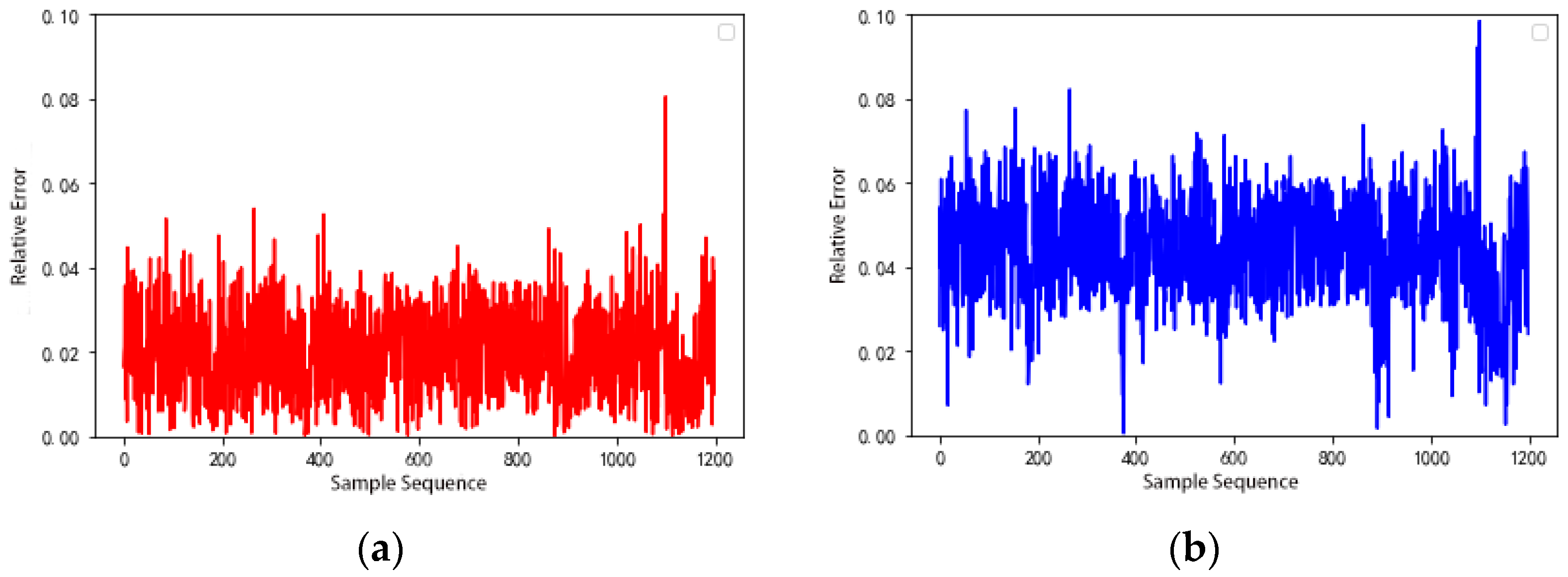
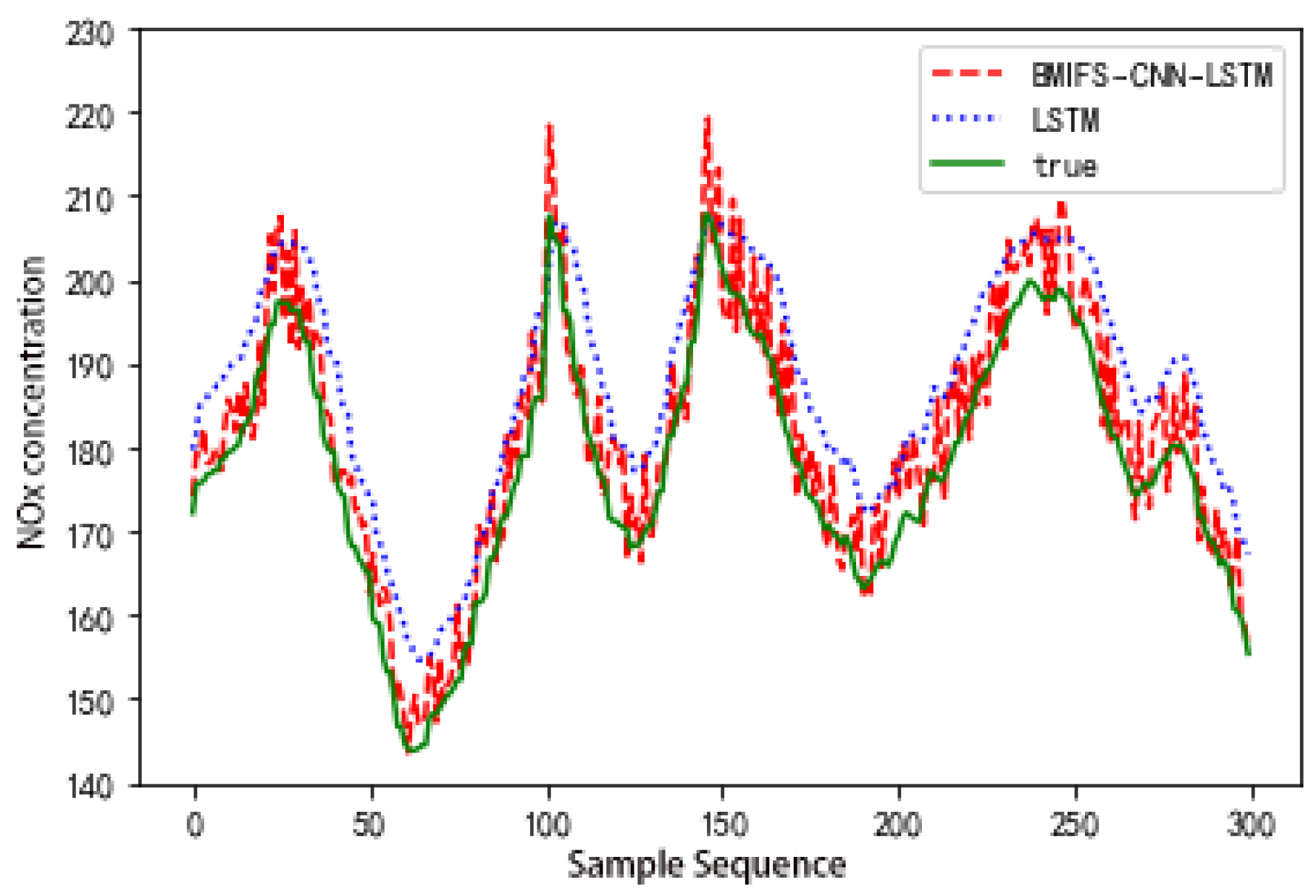
5.2. Forecast Result

When using the Keras framework for LSTM network building, it is necessary to set the necessary parameters, and the final characteristics presented by the model differ depending on the parameter settings. Parameter optimization is the process of selecting an optimal set of parameters for the learning algorithm. In the Keras framework, the parameters that need to be adjusted include the number of neural network layers, the number of neurons in the hidden layer, the total number of training sessions, the batch sample size, the learning rate, among others. In this paper, for the LSTM prediction model, the two parameters of total number of training and learning rate are mainly tuned.

It is found that the accuracy gradually converges when the training reaches about 1000 times, and the accuracy decreases significantly after the number reaches about 9000 times, which is mainly due to the gradient explosion caused by too much training. Therefore, by setting the number of training sessions to 2000, the network model can be trained in less time while avoiding the gradient explosion. With learning rates of 0.001, 0.003, and 0.006, the accuracy of the model is consistent up to 5000 training sessions, but the curve with a learning rate of 0.001 decreases more significantly after 5000 training sessions, and the curve with a learning rate of 0.006 also decreases significantly after 6800 training sessions. To a certain extent, the size of the learning rate determines the speed of updating the parameters to the optimal value. From the analysis of the experimental results, we know that when the learning rate is too large, the gradient step of the model is too large for each training, and the optimal solution is easily missed.

After several experiments to adjust the parameters, the learning rate of Adam’s algorithm is set as 0.003. The number of batch samples is 50. The number of LSTM network layers is 2. The number of neurons in the hidden layer is 100, and the number of training times is set as 2000. The preprocessed 1600 sets of data, 80% of which were used as the training data for the model and 20% as the test data of the model, were used to build the LSTM network model without auxiliary variables extraction and the LSTM network model with auxiliary variables screening. The final model-training-data fitting effect is shown in Figure 6, and the relative errors are shown in Figure 7a,b.

According to Figure 6, it can be seen that the two types of models can fit the training data better, but from the relative errors shown in Figure 7a,b, it can be seen that the left model has a smaller error than the right model, so it can be concluded that the samples selected in advance by the BMIFS auxiliary variables can better train the model, so as to achieve a better fitting effect.

Next, the trained model is used to estimate the test data, and obtain the final estimated results and errors of the two types of models, as shown in Figure 8 and Figure 9a,b.

According to Figure 8, it can be analyzed and found that the prediction accuracy of the prediction model without auxiliary variable extraction is not as high as that of the prediction model with auxiliary variable extraction. Combined with the results shown in Figure 9a,b, it can be further found that the prediction based on BMIFS-LSTM gives a relative error of the model that is smaller in comparison, which further shows that the prediction accuracy of the model is higher.

The error descriptions of the two types of prediction models are shown in

Table 3. Comparison table of simulation results.

Model	MRE (%)	RMSE
BMIFS-LSTM training model	0.0246	1.3715
LSTM training model	0.0458	2.2024
BMIFS-LSTM test model	0.0297	1.5237
LSTM test model	0.0643	3.0251

.

The addition of CNN for automatic feature extraction in addition to the original LSTM model can greatly improve model accuracy and training speed. The total training time of LSTM model is 340 s, while the total training time of BMIFS-CNN-LSTM is only 86 s, and its final prediction is shown in Figure 10 with the relative error given in Figure 11.

The BMIFS-CNN-LSTM model is compared with the model without CNN feature extraction in the following experimental analysis. Statistically, the errors of the two types of models are shown in

Table 4. Comparison of model error statistics.

Models	Average Relative Error (%)	Root Mean Square Error
BMIFS-LSTM Prediction Model	0.0297	1.5237
BMIFS-CNN-LSTM Prediction Model	0.0126	1.0113

.

In summary, compared with the BMIFS-LSTM model, the BMIFS-CNN-LSTM model has a lower average relative error and root mean square error, and the model training time is shorter. The rationality of introducing CNN automatic feature extraction is demonstrated. Meanwhile, compared with the traditional long short-term memory neural network (LSTM), the LSTM algorithm with the introduction of the improved mutual information feature selection algorithm (BMIFS) has a lower average relative error of 3.45% and a lower root mean square error of 1.50, which indicates a better prediction of NOX concentration at the SCR inlet and effectively solves the problem of delay in NOx concentration measurement.

6. Conclusions

At present, most thermal power plants use selective catalytic reduction (SCR) technology to reduce NOx emissions, using automatic flue gas monitoring systems to measure NOx concentration in real time and combine the measurement results to select the optimal amount of ammonia injection for denitrification treatment. However, the system has a large delay in making measurements and cannot accurately reflect the real-time changes in the NOx concentration at the SCR inlet when the unit load fluctuates frequently, thus failing to guide the reactor action in a timely manner. In response, this paper establishes an SCR inlet NOx concentration prediction algorithm based on BMIFS-LSTM. A modified mutual information feature selection algorithm (BMIFS) is used to screen seven auxiliary variables such as unit load and total secondary air, and the dominant variables are input into a long short-term memory neural network (LSTM) together with the auxiliary variables to establish a BMIFS-LSTM prediction model. To verify, the historical operation data of a 300 MW thermal power unit are used for simulation experiments. The experimental results show that the model reduces the average relative error by 3.45% and the root mean square error by 1.50, compared with the LSTM model without auxiliary variable screening. The prediction results have less deviation and higher accuracy, and have better prediction effect on the NOX concentration at the SCR inlet. The problem of delay in NOx concentration measurement is solved, which effectively reduces the occurrence of environmental pollution problems such as ammonia escape and NOX emission overload.

References

1. Zhong, J. The Economics of Low-NOx Technology and the Exploration of New Low-NOx Control Technology; Zhejiang University: Hangzhou, China, 2006. [Google Scholar]
2. Li, Y.; Huang, W.; Xi, J. Power plant NO_x emission prediction based on Stacking algorithm integration model. Therm. Energy Power Eng. 2021, 36, 73–81. [Google Scholar] [CrossRef]
3. Liu, K.; Wei, B.; Chen, L.; Wang, J.; Li, J.; Liu, J. Influence of low-load flue gas recirculation on combustion and NOx emissions of pulverized coal boilers. Chin. J. Power Eng. 2021, 41, 345–349, 379. [Google Scholar]
4. Hochreiter, S.; Schmidhuber, J. Long short-term memory. Neural Comput. 1997, 9, 1735–1780. [Google Scholar] [CrossRef]
5. Kingma, D.; Ba, J. Adam: A method for stochastic optimization. arXiv 2014, arXiv:1412.6980. [Google Scholar]
6. Verma, S.; Singh, S.; Majumdar, A. Multi-label LSTM autoencoder for non-intrusive appliance load monitoring. Electr. Power Syst. Res. 2021, 199, 107414. [Google Scholar] [CrossRef]
7. Wu, P.; Luo, L. Prediction of ship motion trajectory based on RNN-LSTM. Shipbuild. Technol. 2021, 49, 11–16. [Google Scholar]
8. Xiang, Z. Confidence Interval Prediction of Smart Grid Link Quality Based on LSTM. Electrical Measurement and Instrumentation. pp. 1–10. Available online: http://kns.cnki.net/kcms/detail/23.1202.TH.20210623.0948.004.html (accessed on 4 July 2021).
9. Zhao, Y. Power data analysis method combining GA and LSTM network. Electron. Des. Eng. 2021, 29, 161–165. [Google Scholar]
10. Song, S.; Li, B. Research on short-term prediction method of photovoltaic power generation based on LSTM network. Renew. Energy 2021, 39, 594–602. [Google Scholar]
11. Chen, C.; Wang, X.; Liang, J.; Ma, W. LSTM photovoltaic power generation prediction method based on a new attention mechanism. Mod. Comput. 2021, 11, 28–32+38. [Google Scholar]
12. Zhang, Z. Research on Spacecraft Time Series Prediction Method Based on LSTM; Beijing Jiaotong University: Beijing, China, 2020. [Google Scholar]
13. Zheng, T. Near-Space Hypersonic Target Track Estimation and Prediction Based on Recurrent Neural Network; Harbin Institute of Technology: Harbin, China, 2020. [Google Scholar]
14. Hu, D.; Meng, X.; Lu, S.; Xing, L. The application of a parallel LSTM-FCN model in ship trajectory prediction. Control Decis. 2021, 4, 1–7. [Google Scholar] [CrossRef]
15. Yang, B. Research and Application of Ship Trajectory Analysis Based on AIS; University of Electronic Science and Technology of China: Chengdu, China, 2018. [Google Scholar]
16. Lu, J.; Song, S.; Jing, Y.; Zhang, Y.; Gu, L.; Lu, F.; Hu, Z.; Li, S. Fundamental Frequency Detection of Underwater Moving Target Noise Based on DEMON Spectrum and LSTM Network. Applied Acoustics. pp. 1–11. Available online: http://kns.cnki.net/kcms/detail/11.2121.o4.20210621.1436.006.html (accessed on 4 July 2021).
17. Ding, C. Planning of RMB Exchange Rate Prediction Scheme Based on Multi-Time Scale CNN-LSTM Neural Network; Shanghai Normal University: Shanghai, China, 2021. [Google Scholar]
18. Tian, Y. Research on Stock Price Trend Prediction Based on Investor Sentiment and LSTM; Shanghai Normal University: Shanghai, China, 2021. [Google Scholar]
19. Wei, Q.; Chen, S.; Tan, Z.; Huang, W.; Ma, G. Based on SA-LSTM, the dynamic lag relationship between hydropower stations. Hydropower Energy Sci. 2021, 39, 16–19. [Google Scholar]
20. Zhang, D. Research on Optimization Technology of Large-Scale Reservoir Water Temperature Regulation Based on Artificial Intelligence Algorithm; China Institute of Water Resources and Hydropower Research: Beijing, China, 2020. [Google Scholar]
21. Sun, B.M.; Wang, D.H.; Yang, B.; Zhang, S.H.; Kong, L.Y. Prediction Model for the Boiler NOx Emission with Material Properties Based on the Artificial Neural Network. Adv. Mater. Res. 2013, 676, 40–45. [Google Scholar] [CrossRef]
22. Li, X.; Xu, G. Wind power generation power prediction method based on long short-term memory neural network. Power Gener. Technol. 2019, 40, 426–433. [Google Scholar]
23. Zhai, Y.; Xu, L.; Ji, X.; Ji, H.; Wang, J.; Sha, Y. Short-term load forecasting based on long and short-term memory neural network. Inf. Technol. 2019, 10, 27–31. [Google Scholar]
24. Mao, X.; Tan, J.; Yao, Y.; Li, B.; Wu, C. Saturated load forecasting method and application based on long and short-term memory neural network. Hydropower Energy Sci. 2019, 37, 192–195+168. [Google Scholar]
25. Tang, Z.; Zhao, G.; Cao, S.; Zhao, B. Ultra-short-term wind direction prediction based on SWLSTM algorithm. Chin. J. Electr. Eng. 2019, 39, 4459–4468. [Google Scholar]
26. Peng, H.; Long, F.; Ding, C. Feature selection based on mutual information criteria of max-dependency, max-relevance, and min-redundancy. IEEE Trans. Pattern Anal. Mach. Intell. 2005, 27, 1226–1238. [Google Scholar] [CrossRef] [PubMed]
Figure 1. Overall research process flow chart.
Atmosphere 13 00686 g001
Figure 2. Schematic diagram of pulverized coal combustion.
Atmosphere 13 00686 g002
Figure 3. CNN-LSTM network architecture.
Atmosphere 13 00686 g003
Figure 4. LSTM network input and output.
Atmosphere 13 00686 g004
Figure 5. Model flow chart.
Atmosphere 13 00686 g005
Figure 6. Comparison chart of training-data fitting effect.
Atmosphere 13 00686 g006
Figure 7. (a) Training-data estimation error. (b) Training-data estimation error.
Atmosphere 13 00686 g007
Figure 8. Comparison chart of estimated effect of test data.
Atmosphere 13 00686 g008
Figure 9. (a) Estimated error of test data. (b) Estimated error of test data.
Atmosphere 13 00686 g009
Figure 10. BMIFS-CNN-LSTM images of predicted and actual values.
Atmosphere 13 00686 g010
Figure 11. Error curve chart.
Atmosphere 13 00686 g011