Short-Term Intensive Rainfall Forecasting Model Based on a Hierarchical Dynamic Graph Network

Abstract

Accurate short-term forecasting of intensive rainfall has high practical value but remains difficult to achieve. Based on deep learning and spatial–temporal sequence predictions, this paper proposes a hierarchical dynamic graph network. To fully model the correlations among data, the model uses a dynamically constructed graph convolution operator to model the spatial correlation, a recurrent structure to model the time correlation, and a hierarchical architecture built with graph pooling to extract and fuse multi-level feature spaces. Experiments on two datasets, based on the measured cumulative rainfall data at a ground station in Fujian Province, China, and the corresponding numerical weather grid product, show that this method can model various correlations among data more effectively than the baseline methods, achieving further improvements owing to reversed sequence enhancement and low-rainfall sequence removal.

1. Introduction

Short-term intensive rainfall is generally defined as a cloudburst event in which the accumulated rainfall reaches or exceeds 30 mm within 3 h (Fujian Provincial Meteorological Observatory) [1]. It is usually caused by strong convective weather and is characterized by extreme suddenness, high destructiveness, and a short duration. It can easily cause natural disasters such as mountain torrents, mudslides, and urban floods. The forecasting accuracy of short-term intensive rainfall is usually lower than that of ordinary rainfall events in China [2]. Inaccurate forecasts may lead to a serious loss of life and property. Therefore, improving the accuracy of short-term forecasting is important.

We focus on two types of short-term intensive rainfall forecasting methods [3]. The radar extrapolation method uses historical radar echo maps with a high spatial–temporal resolution, as drawn by meteorological radars, to forecast the rain and cloud movement. It uses the optical flow method [4], precipitation cloud extrapolation [5], or other methods [6] to predict the movement. In addition, it subsequently uses rainfall rate–reflectivity relationships or other means to invert the results into rainfall data. The Numerical Weather Prediction (NWP) method, based on historically accumulated observation data, uses numerical calculations to solve the fluid mechanics and thermodynamic equations that represent the weather evolution under certain conditions. The result is a computer-simulated NWP product. Based on this, forecasters combine various monitoring products and their own experience to conduct comprehensive analyses and corrections, thus finally obtaining forecasting results.

With the increased scale of deployment of metering equipment and meteorological data expansion, previous studies have integrated deep learning with meteorological forecasting methods. Recent extrapolation methods transform the problem into a video-like prediction, such that it is easier to model the long-range spatial–temporal relationship when compared with that in traditional methods [7]. Some attempts have focused on using the NWP products as input data for deep learning methods to perform prediction tasks [8,9].

However, forecasting short-term intensive rainfall using deep learning still faces challenges: (1) the distribution of meteorological data is complex and involves multi-modal dynamics, which are difficult to model; (2) statistics show that samples have a robust scale-free structure in the atmospheric rainfall field [10], which indicates a data imbalance problem; (3) when using data with a temporal resolution of 3 h, modeling is more difficult than radar extrapolation at high spatial–temporal resolutions and small neighborhood variations; and (4) NWP products are not the actual measured results, as their accuracy is limited by the characteristics of the models they use.

To manage these challenges, based on our previous study [1], we combined rainfall data from ground stations and related data from an NWP product to propose the Hierarchical Dynamic Graph Network (HDGN), a new model based on spatial–temporal sequence prediction and a Graph Convolutional Network (GCN). By designing the corresponding structure, we comprehensively captured the correlations among time, space, and features, which facilitated the prediction of short-term intensive rainfall.

The remainder of this paper is organized as follows. Section 2 introduces the background related to this study, including the NWP, spatial–temporal sequence prediction, study area, and data sources. Section 3 presents the methods applied for short-term intensive rainfall prediction, which involve data preprocessing and the HDGN model. Section 4 presents the configuration of the experiments and interpretations of their results. Section 5 provides the conclusions of the study.

2. Background

2.1. Numerical Weather Prediction

Multi-scale forecasts are provided by operational NWP centers, which involve small to planetary-scale emulations at time resolutions from the minute to seasonal scale. The numerical calculation model in the NWP is frequently updated with the aid of new observation data and forecasting technologies, thereby improving the physical simulation performance and uncertainty quantification of the model. This also improves the effect of model forecasting and data assimilation.

We used fine-grid numerical forecasting products from the European Centre for Medium-Range Weather Forecasts (ECMWF) and the Weather Research and Forecasting (WRF) method, a unified mesoscale weather-forecasting model.

However, NWP has certain limitations related to the cumulative error resulting from the high complexity of the simulation process. The ECMWF is disadvantageously characterized by a weak intensity forecast [11]. The WRF model performs relatively poorly when estimating the rainfall value [12]; its rainfall forecasting results may not be as optimal as those of the ECMWF [13]. Generally, the performance of the NWP in the convective period of a precipitation forecast is relatively poor, despite the occurrence of short-term intensive rainfall during the convective period. The lifetime of convective storm cells is generally <30 min [14], such that it is difficult to accurately predict short-term intensive rainfall events using a single NWP simulation. In this study, we combined the measured cumulative rainfall data from ground stations and related data from the NWP product on the input side to overcome the limitations associated with a single set of NWP data. Additionally, based on these data, the concept of spatial–temporal sequence prediction was employed to predict future rainfall conditions.

2.2. Spatial–Temporal Sequence Prediction

As a sub-field of deep learning, spatial–temporal sequence prediction is suitable for uncovering the spatial–temporal correlations among data, such as rainfall-related information for forecasting tasks based on time-sequence prediction. Classical models for time-sequence prediction include Long Short-Term Memory (LSTM) [15], which is a recurrent neural network with long- and short-term memory cells, and the Deep Belief Network (DBN) [16], which is a multi-layered probabilistic generative neural network. They have a simple structure with a low cost; however, they are poor in integrating spatial information from our data. To enhance the performances of these methods, we can classify the spatial–temporal sequence prediction problems into grid and non-grid scenarios [17].

Grid spatial–temporal sequence prediction uses fixed space coordinates to characterize the spatial–temporal relationship among data [18,19,20]. Convolutional LSTM (ConvLSTM) [21] combines LSTM and a three-dimensional (3-D) convolutional neural network [22], which is a deep learning network for extracting information from spatial data. It is portable and can be the building block of a predictive network, but it lacks bidirectional information flow between the different layers in the temporal direction. Sequence-to-Sequence (Seq2Seq) [23] is a basic recurrent architecture used in our model to perform frame-by-frame predictions. PhyDNet [24] uses an encoder–predictor–decoder architecture, which includes the mutual conversion of data and physical feature spaces. Furthermore, a previous study developed a video prediction model based on a multi-level feature space [25]; our study extends this idea to the graph domain. Multi-level feature spaces increase the model complexity but facilitate the extraction of feature correlations among data. Finally, a model for serially generating two-dimensional (2-D) convolutional kernels, with a sliding window [26], inspired this study regarding the hierarchical generation of graph convolution operators.

Non-grid spatial–temporal sequence prediction uses additional structures, such as graphs (a structure composed of nodes and edges), to characterize the spatial–temporal relationships among data [27,28,29]. The Attention-based Spatial–Temporal Graph Convolutional Network (ASTGCN) [30] alternately calculates the temporal and spatial attention within the data, which act as antecedent auxiliary transformations to the graph convolution operator. However, its high cost of spatial attention prevents it from being used in large graphs, where ours can be used. The Spatial–Temporal Graph Ordinary Differential Equation (STGODE) network [31] models the semantic adjacency matrix of a graph via the dynamic time-warping algorithm. Graph Convolution embedded LSTM (GC-LSTM) [32] uses the Inverse Distance Weight (IDW) to calculate the weights of a graph; the graph convolution operator selects one- to K-hop neighbors. In the HDGN, we also use semantic distances, which are more indicative of the correlations between node pairs, as weights instead of fixed geographical distance, and this method can increase the model dynamics at a low cost. Our graph convolution operator has the same capabilities as those of the GC-LSTM. The Dynamic Graph Convolutional Recurrent Network (DGCRN) [33] uses a highly dynamic graph construction method, whereas we proposed a hierarchical graph generation process; compared to the previous method, our approach trades a small reduction in flexibility for a faster graph construction speed.

2.3. Study Area and Data Sources

Fujian Province is located in Southeastern China, with a total land area of 12.4 million km². It has a subtropical maritime monsoon climate characterized by an average annual temperature of 15.0 to 21.7 °C, with hot summers and warm winters; its annual precipitation ranges from 1132 to 2059 mm, where March to September accounts for 81.4% of the annual precipitation. The topography of Fujian is high in the northwest and low in the southeast. It has two mountain belts that trend from the northeast to the southwest: the Wuyi Mountains in northwestern Fujian and the Jiufeng and Daiyun mountains in northeastern to central Fujian. Owing to the influence of the terrain, these areas are the centers of heavy rainfall in Fujian [34]. Figure 1 depicts the occurrence of short-term intensive rainfall in Fujian from February 2015 to December 2018. Fujian is one of the areas of high-frequency intensive rainfall in China, which often leads to severe flooding and geological hazards.

The four original datasets issued by the Fujian Meteorological Observatory were used in this study (see

Table 1. Details of the original datasets.

Dataset	Stations	ECMWF250	ECMWF125	WRF
Horizontal range	23.52°–28.37° N, 115.84°–120.67° E	23.5°–28.5° N, 115.5°–121.0° E		23.5°–28.45° N, 115.5°–120.99° E
Time range	February 2015 to December 2018			January 2017 to December 2018
Time resolution	3 h			1 h
Number of stations/grid points	2170	23 × 21	45 × 41	62 × 56
Grid spacing	—	0.25° × 0.25°	0.125° × 0.125°	0.09° × 0.09°
Number of available features	3	113	26	24
Starting time of the forecast	—	08:00 and 20:00 (UTC + 8)

for details); the grid points refer to a series of nodes arranged in rows (latitude) and columns (longitude). These datasets can be divided into three categories.

Stations: A dataset of the observed rainfall, comprising data collected by 2170 available ground stations in Fujian. It contains three features, i.e., the longitude, latitude, and measured 3 h accumulated rainfall.

ECMWF: It comprises the ECMWF250 and ECMWF125 datasets for Fujian. With the exception of a few features, such as the dew point temperature, their feature sets do not overlap with each other.

WRF: A dataset containing the Fujian WRF grid data, which is divided into 3-h interval groups; only the forecasting results from the third hour were used for alignment with the other datasets.

3. Methodology

3.1. Problem Description

Let the data obtained from the samplings performed at equal time intervals belong to one frame. We set sequence prediction as the task of outputting the predicted sequence data as close as possible to the ground truth based on the historical data, which can be expressed as follows:

$$\{X_0,\dots ,X_{T_{in}-1}\}\to \{X_{T_{in}},\dots ,X_{T_{in}+T_{out}-1}\},$$

(1)

where $X$ represents a frame, and $T_{in}$ and $T_{out}$ represent the historical and predicted sequence lengths, respectively.

The structure of $X$ differs for different types of prediction problems. $X\in {ℝ}^F$ represents the time-sequence prediction, $X\in {ℝ}^{N\times F}$ represents the non-grid spatial–temporal sequence prediction, and $X\in {ℝ}^{M\times F}$ represents grid prediction, where $F$, $N$, and $M$ denote the number of features, nodes, and measurement dimensions of the grid, respectively. When the grid is 2-D, $M=H\times W$, where $H$ and $W$ represent the height and width of the grid, respectively.

We set our object as a non-grid spatial–temporal sequence prediction problem, where $X_{t,0}=X_t$ in the HDGN. The grid spatial–temporal sequence prediction was applied after separating the latitude and longitude coordinates from the data points. The time-sequence prediction methods can individually predict each node and then combine them.

3.2. Data Preprocessing

For the stations dataset, we used the IDW interpolation method [35] on each frame to interpolate the rainfall values to the ECMWF250 and WRF grid points. Thus, the measured cumulative rainfall and corresponding NWP features shared identical spatial coordinates, which avoided forecasting difficulties caused by a lack of measured rainfall data. The station dataset is important because the model will perform poorly if the percentage of missing values is high. In this context, the observed rainfall data must usually be obtained from multiple sources to prevent potential problems caused by missing data when the data are obtained from a single source.

For the NWP datasets, we used the forecasting period between 12 and 33 h owing to numerical instability in the first 12 h of the NWPs. We then selected the forecasting data closest to the start time to reduce the influence of long-term forecasting errors. Because each feature has a different impact on network training and prediction performance, the Box Difference Index (BDI) was used for feature selection [36] to reduce the volume of data and avoid feature overlap. The higher the index, the stronger the feature’s ability to distinguish whether the data point was a short-term intensive rainfall event. The BDI of each feature was calculated as follows:

$$BDI=\frac{\left|m_{30}-m_0\right|}{{\sigma }_{30}+{\sigma }_0},$$

(2)

where $m_0$ and $m_{30}$ represent the characteristic mean values of the rainfall for data points between 0 and 30 and above 30 mm, respectively, and ${\sigma }_0$ and ${\sigma }_{30}$ represent the standard deviations of the rainfall values for the data points between 0 and 30 mm and above 30 mm, respectively. After calculation, a list of each feature in descending order of BDI value was obtained, and the features with the highest BDI were selected in turn. Note that features with a high percentage of missing data owing to equipment failure, etc., were not used because they degrade the performance of the model; therefore, we manually skipped these features and replaced them with features with lower BDIs.

Table 2. Description of the selected features.

Data Source	Feature Name	Meaning
ECMWF125	Q_850	Specific humidity 850 kPa
	Ki	k index
	Td_850	Dew point temperature 850 kPa
	GH_1000	Geopotential height 1000 kPa
	Tt_850	Temperature 850 kPa
ECMWF250	TCWV	Atmospheric water vapor content
	MSL	Sea-level pressure
	2D	Dew point temperature 2 m
WRF	TCDC	Total cloud cover
	RH_850	Relative humidity 850 kPa
	LCDC	Low cloud cover
	CR	Combined reflectance
	GUST	Wind gust
	CAPE	Convective avail pot energy
	REFD_1000	Radar-derived reflectivity 1000 kPa
	MSLP	Mean sea-level pressure

lists the features that we selected following the above process and used in the subsequent steps.

After feature selection, we constructed the sequential datasets adapted to the HDGN and other sequence prediction models, i.e., S-ECMWF and S-WRF, where S denotes the sequence. Their construction methods are shown below: (1) As the ECMWF dataset comprises two groups of data with different grid spacings, they must be merged. The selected ECMWF125 retained only the features of the 23 × 21 grid points that overlapped with ECMWF250. The features of both were then concatenated according to the grid points. (2) The interpolated rainfall data were spliced into the two datasets using the operation described in (1). (3) Linear interpolation was used to supplement the missing values. The data were standardized with the z-score. (4) Sequence samples were generated using a sliding window with a step size of one frame. (5) The graph, $G_0$, was constructed according to the grid of the data, where each grid point was treated as a node and each node formed an edge with the nearest node in eight directions (N, E, S, W, NE, SE, SW, and NW); a direction with no nodes in it was skipped. Graphs in the HDGN were stored as a compressed sparse matrix structured as ${ℝ}^{2\times E}$, where $E$ represents the number of edges in the graph. The edges of the graphs in the HDGN were all undirected edges, unless otherwise specified. (6) S-ECMWF and S-WRF contained the sequence samples and $G_0$, respectively.

As an optional step, we performed data augmentation on the S-ECMWF and S-WRF datasets before training to improve the prediction performance. This involved two methods: (1) Reversed sequence enhancement: the reverse form, $\{X_{T_{in}-1},\dots ,X_0\}$, of the historical sequence, $\{X_0,\dots ,X_{T_{in}-1}\}$, was generated and added to the training data; the related sequence prediction task is shown in Equation (3). (2) Low-rainfall sequence removal: 10% of the training samples with the highest number of data points characterized by zero rainfall in the historical sequence were removed. This configuration was used unless otherwise specified.

$$\{X_{T_{in}-1},\dots ,X_0\}\to \{X_{-1},\dots ,X_{-T_{out}}\}$$

(3)

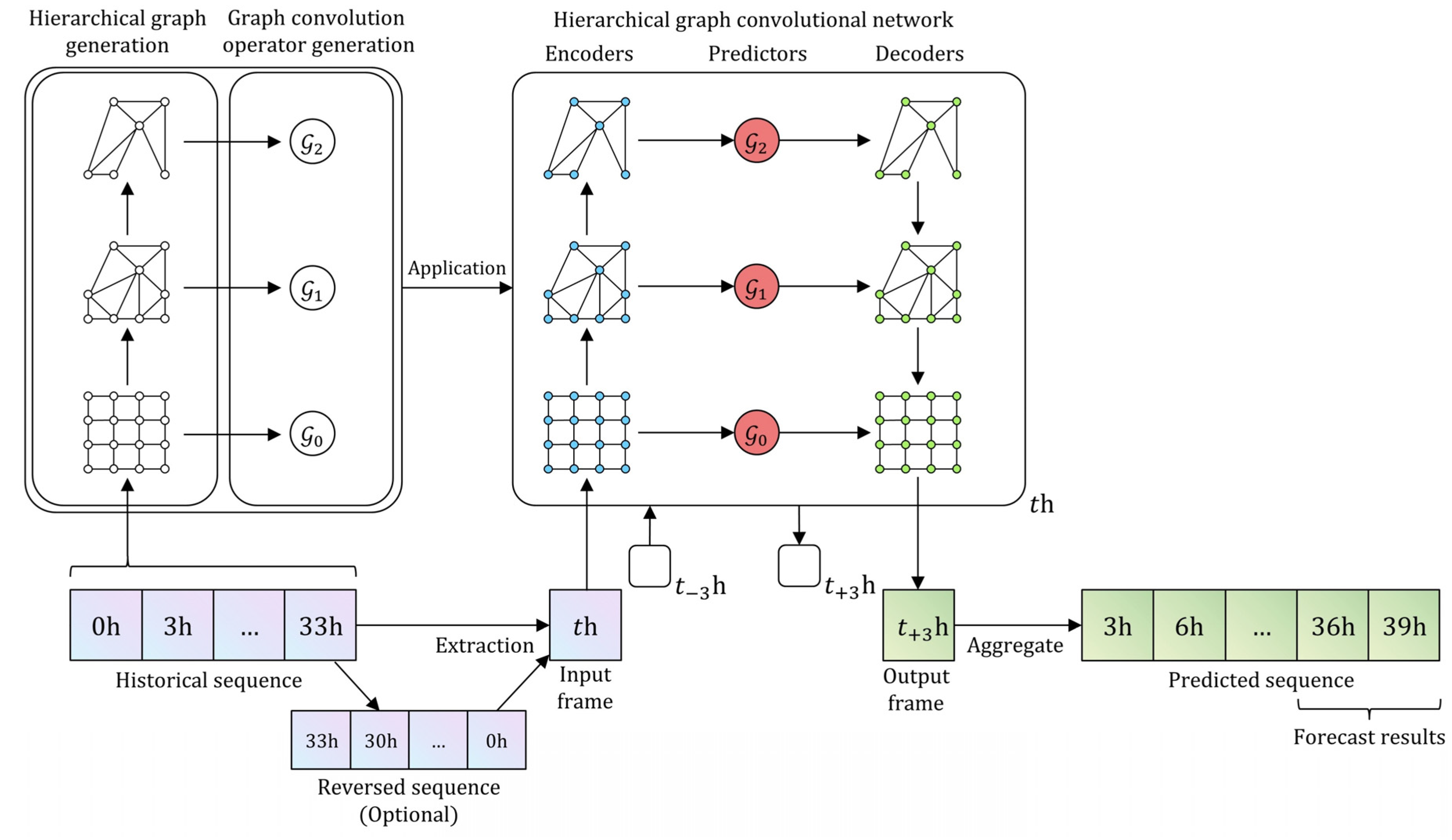
3.3. Hierarchical Dynamic Graph Network

We proposed an HDGN model for short-term intensive rainfall forecasting, which is shown in Figure 2. We note that the structure of the Hierarchical Graph Convolutional Network (HGCN) should correspond to the hierarchical graph generation process. The components of this model were implemented based on Multi-Layer Perceptron (MLP), a trivial forward-structured artificial neural network, unless otherwise specified.

The steps of the sequence prediction were as follows. (1) The model read a historical sequence and generated multi-level graphs based on it. It then generated the corresponding graph convolution operators based on these graphs, finally using these results to initialize the HGCN. (2) The HGCN read each frame on the historical sequence in chronological order and output the corresponding predicted frames while updating its own state. When the HGCN reached the end of the historical sequence, the last predicted frame was re-input into the HGCN as the historical frame such that continuous prediction could be achieved. (3) The model output the forecasting results for this historical sequence.

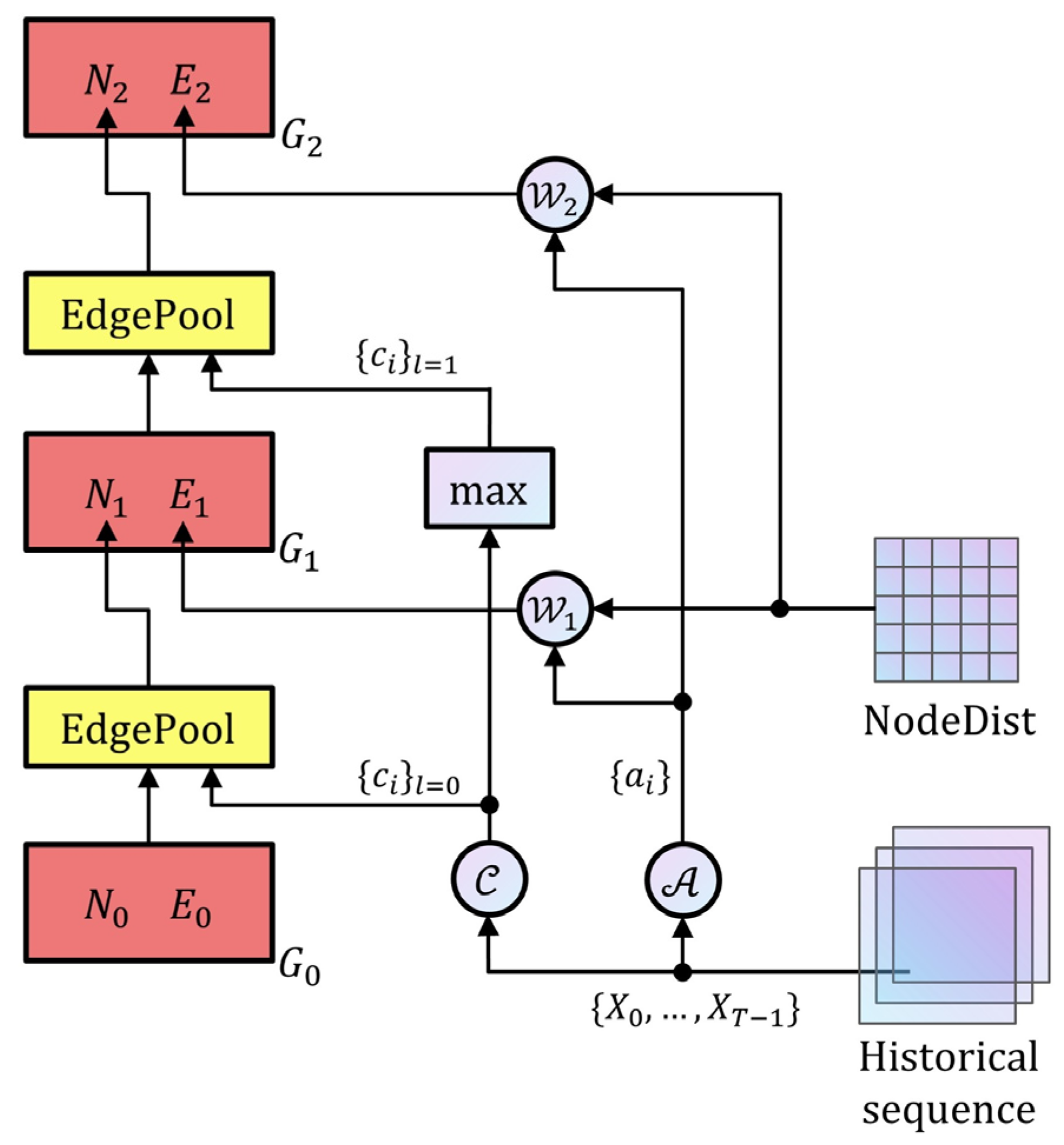
3.3.1. Hierarchical Graph Generation

Graph pooling was used to dynamically construct multi-level graphs, which serve as the basis for the subsequent steps. Figure 3 shows the process of hierarchical graph generation.

We used a set of MLP encoders, $\mathcal{C}$, $\mathcal{A}$, and $\mathcal{W}$, to extract the auxiliary information according to the historical sequence. Each node cluster feature was $c_i$, $i\in \left\{0,\dots ,N-1\right\}$, and the edge weight adjustment feature was $a_i$, $i\in \left\{0,\dots ,E-1\right\}$. These were calculated using $\mathcal{C}$ and $\mathcal{A}$.

EdgePool [37] was adopted to generate a new non-weighted graph based on edge shrinking. The related process was as follows. (1) The correlation score of each edge was calculated using Equations (4) and (5), where $\mathrm{concat}$ is the concatenate operation and ${\mathrm{softmax}}_i$ is a normalization function on all adjacent edges of node $i$. (2) The edge with the highest score was shrunk, followed by merging of its two adjacent nodes into a new node with a clustering feature of $\max \left(c_i,c_j\right)$. The adjacent edges of this new node no longer participated in the shrinking of this layer. (3) Step (2) was repeated until all edges were processed. We note that at least 50% of the nodes were always reserved for each pooling. For a graph with numerous nodes, multiple EdgePools were arranged instantaneously to reduce the number of layers.

$$s_{i,j}=\mathrm{MLP}\left(\mathrm{concat}\left(c_i,c_j,e_{i,j}\right)\right)$$

(4)

$$s_{ij}=\max \left(0.5+{\mathrm{softmax}}_i\left(s_{i,j}\right),0.5+{\mathrm{softmax}}_j\left(s_{i,j}\right)\right)$$

(5)

We generated the weights for this new graph using Equation (6), where $d_{i, j}$ is the geographic distance between $i$ and $j$, multiplied by a multiplier for correction. The multiplier allowed learnable weights and aided in the modeling of the semantic distance between the nodes based on $d_{i, j}$. We constrained the multiplier within$\left(0.5, 1.5\right)$by the sigmoid function $\sigma$, to obtain more stable weights.

$$e_{i,j}=d_{i, j}\left(0.5+\sigma \left(\mathcal{W}\left(a_i,a_j\right)\right)\right)$$

(6)

3.3.2. Graph Convolution Operator Generation

Based on a given graph, $G$, we generated a graph convolution operator, $\theta$, using graph Fourier transform theory [38].

First, we calculated the symmetric normalized Laplace matrix of the graph via Equation (7), where $A$ and $D$ are the adjacency and degree matrices of the graph, respectively, and $I$ is the identity matrix corresponding to $A$.

$$L_{sym}=I{D}^{-\frac{1}{2}}A{D}^{-\frac{1}{2}}$$

(7)

Next, eigenvalue decomposition was performed on $L_{sym}$; this step is complex, especially when there are many nodes on the graph. Therefore, the Chebyshev polynomial approximation was used to accelerate the solution process [39]. The graph convolution operator, $\theta$, based on $L_{sym}$, was approximated as a superposition of $K$ parts, with the $k$-th part extracting relevant information from $k$-hop neighbors around the target node, as shown in Equation (8), where ${\lambda }_{max}$ is the maximum eigenvalue of $L_{sym}$ and $T_k$ represents the $k$-th term of the first type of recursive Chebyshev polynomial; i.e., Equation (9), where $T_0\left(X\right)=I$, $T_1\left(X\right)=X$, and ${\theta }_k$ is the $k$-th learnable graph convolution kernel [40]. The value of $K$ is important; if it is small, the graph convolution operator does not have a good mapping ability; if it is large, it causes over-smoothing, i.e., the data on the graph converge rapidly, which severely affects the subsequent process.

$$\theta \left(L_{sym}\right)={\displaystyle \sum }_{k=0}^{K-1}{\theta }_k{T}_k\left(\frac{2L_{sym}}{{\lambda }_{max}-I}\right)$$

(8)

$$T_k\left(X\right)=2X{T}_{k-1}\left(X\right)-T_{k-2}\left(X\right)$$

(9)

In summary, we calculated $\left\{T_0,\dots ,T_{K-1}\right\}$ through $G$, followed by implementation of the graph convolution process.

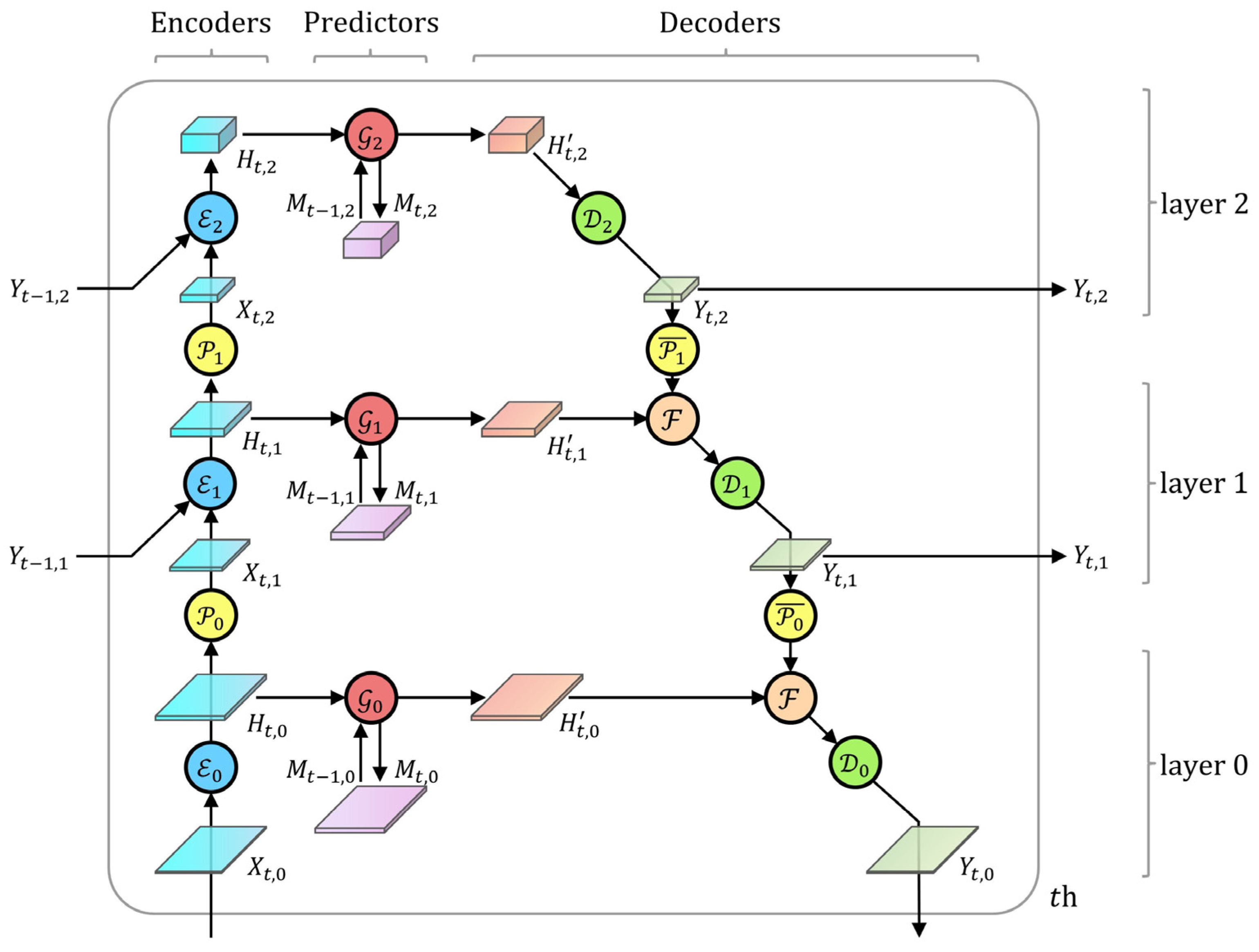
3.3.3. Hierarchical Graph Convolutional Network

We proposed the HGCN, as shown in Figure 4, which is a multi-layered encoder–predictor–decoder network. HGCN extracts the high-level features from the data to produce a multi-level description of the data, which is useful for prediction. A feature space consisted of a set of features used to describe the data. Layer 0 feature space, i.e., the meteorological features within the dataset, and other feature spaces were latent spaces with learnable anonymous features. The encoders were responsible for mapping the low-level feature space to the higher space, whereas the decoders were responsible for performing the opposite process.

The components in the HGCN network are as follows. (1) The encoder, $ℰ$, and decoder, $\mathcal{D}$, map feature spaces to higher- or lower-level hidden spaces through MLP. Based on the residual connection [41], we proposed a cross-frame connection. When $t>0$ and $l>0$, the encoder uses the form shown in Equation (10), where $Y_{t-1,l}$ represents the output feature space of the same layer in the previous frame. The cross-frame connection aids in stabilizing inter-frame and inter-layer information transmission, shortens the transmission path of the high-level information, and alleviates the gradient explosion problem. (2) The predictor, $\mathcal{G}$, communicates information between the nodes in the graph and produces data for the next moment, which are expressed by Equations (11) and (12). $M_{t,l}$ was used to adaptively adjust the update magnitude of $H_{t,l}$, and $M_{-1,l}$ is an empty matrix. $T_{l,k}$ was calculated from $G_l$, $○$ is the element-wise product, and $U_l$, $W_l$, ${\theta }_{l, k}$, $a_l$, and $b_l$ are learnable matrices. (3) Graph data pooling, $\mathcal{P}$, and graph data de-pooling, $\overline{\mathcal{P}}$, convert the data between the graphs in adjacent layers. $\mathcal{P}$ copies the corresponding lower-level node with the largest rainfall as the new node, while $\overline{\mathcal{P}}$ copies the node to every corresponding lower-level node. (4) The fusion operation, $ℱ$, was used to integrate the data, as shown in Equation (13). To avoid learning of constant transformations by the model, we used the maximum function to achieve $ℱ$.

$$H_{t,l}={ℰ}_l\left(\mathrm{concat}\left(Y_{t-1,l},X_{t,l}\right)\right)$$

(10)

$$M_{t,l}=\sigma \left(U_l{M}_{t-1,l}+W_l{H}_{t,l}+a_l\right)$$

(11)

$$H_{t,l}^{\prime }=\left(1-M_{t,l}\right)○H_{t,l}+M_{t,l}○\tan \mathrm{h}\left({\displaystyle \sum }_{k=0}^{K-1}{\theta }_{l, k}{T}_{l, k}{H}_{t,l}+b_l\right)$$

(12)

$$Y_{t,l}^{\prime }=ℱ\left(H_{t,l}^{\prime },Y_{t,l+1}\right).$$

(13)

According tohe number of nodes in the S-ECMWF and S-WRF datasets, we designed the corresponding HGCN structures as shown in Figure 5.

3.3.4. Loss Function

After obtaining the prediction results of the model, a loss function was used to evaluate the degree of difference between the predicted values, $x$, and reference values, $y$, to guide model training. Owing to the imbalance in the rainfall values, we implemented a set of rainfall thresholds, $\varphi =\left\{0.1,1,5,10,20,30\right\}$, and grouped all data points into seven categories. The weighted mean absolute error was used as the loss function.

$$loss=\frac{1}{N}{\displaystyle \sum }_{i\in \Omega }\frac{\Omega }{{\Omega }_k}\left|x_i-y_i\right|,$$

(14)

where $\Omega$ represents the total number of data points involved in the evaluation and ${\Omega }_k$ represents the number of the $k$-th category, i.e., within the $i$-th data point. Categories with smaller sample sizes had larger proportions of the prediction error.

4. Experimental Settings and Results

4.1. Experimental Settings

4.1.1. Model Configuration

We implemented the HDGN model on PyTorch [42] 1.6.0 using an NVIDIA Tesla P100-PCIE-16 GB GPU for experiments on a Windows workstation. After shuffling the order of the sequence of samples in the S-ECMWF and S-WRF datasets, they were grouped into three subsets: training, validation, and test sets at a ratio of 6:2:2. For all prediction tasks, the length of the historical input sequence was 12 frames (spanning 36 h) and the length of the forecasting results was 2 frames (spanning 6 h). In the training phase, the model used an Adam optimizer: the initial learning rate was set to 0.0005; early stopping was configured, which could adaptively adjust the learning rate during the training process and stop training when the loss could not be reduced further. The batch size was set to 80 or 12, the number of layers was set to 4, and the term of the Chebyshev polynomial, $K$, was set to 3. We fixed the parameters of the model for the validation and test phases; the validation phase fine-tuned the parameters and the test phase output the evaluation indicators for the forecasting results.

The selection of these hyperparameters was influenced by various aspects. If the length of the historical sequence was short, it was difficult for the model to obtain sufficient information, whereas longer sequences did not significantly improve the prediction effect but increased the time and space cost of the model. The effect of the initial learning rate was reduced after configuring early stopping. A larger batch size could accelerate model training; owing to the large scale of the S-WRF dataset, the upper limit of the GPU load, i.e., 12, was selected. Model performance degraded when $K$ was 2 or 4. The number of layers could significantly affect the prediction accuracy (see Section 4.2.3 for details).

4.1.2. Evaluation Index

We mainly focused on the classification performance of short-term intensive rainfall events. Rainfall evaluation indicators were based on the following three categories of statistical scoring methods: (1) Critical Success Index (CSI), which is a commonly used indicator to measure the rainfall forecasting results. Its values range from $\left[0, 1\right]$; the higher the value, the better the result. (2) Equitable Threat Score (ETS), which is used to measure the degree of improvement in the rainfall forecasting results relative to random forecasting results under the same configuration. Its values range from $\left[-1/3, 1\right]$; the higher the value, the better the result. An ETS of 0 indicates that the model’s prediction results are comparable to random results, whereas ETS ≤ 0 is not acceptable. (3) False Alarm Ratio (FAR), which is the proportion of misclassified data included in the prediction results. Its values range from of $\left[0, 1\right]$; the lower the value, the better the result.

Table 3. Rainfall classification table.

Actual Class	Predicted Class
	0–1 mm	1–30 mm	>30 mm
0–1 mm	$D$	$B_1$	$B_2$
1–30 mm	$C_1$	$A_1$	$B_2$
>30 mm	$C_2$	$C_2$	$A_2$

presents the rainfall classification with 1 and 30 mm as the threshold.

With 1–30 mm as the first category and >30 mm as the second category, the indicators for each category were calculated as follows:

$$CS{I}_k=\frac{A_k}{A_k+{\displaystyle \sum }{B}_k+{\displaystyle \sum }{C}_k},$$

(15)

$$ET{S}_k=\frac{A_k-R_k}{A_k+{\displaystyle \sum }{B}_k+{\displaystyle \sum }{C}_k-R_k},$$

(16)

$$FA{R}_k=\frac{{\displaystyle \sum }{B}_k}{A_k+{\displaystyle \sum }{B}_k},$$

(17)

where $A$, $B$, $C$, and $D$ represent the number of event hits, empty reports, missed reports, and number of successful predictions of non-events, respectively, and $R$ represents the result of the random forecasting model evaluated as follows:

$$R_k=\frac{(A_k+{\displaystyle \sum }{B}_k)(A_k+{\displaystyle \sum }{C}_k)}{A_k+{\displaystyle \sum }{B}_k+{\displaystyle \sum }{C}_k+D}.$$

(18)

We referred to each indicator with a $k$ of 1 as a type 1 indicator and that with a $k$ of 2 as a type 2 indicator. The CSI₂ and ETS₂ indicators generally had values <0.1 in Fujian; values >0.1 were considered major breakthroughs. Repeated comparison experiments revealed that for each deep learning method considered herein, the first four decimal places of the type 2 indictors remained unchanged, while the subsequent decimal places showed fluctuations; thus, we retained only the initial four decimal digits to make the results reasonable. Because of the same reasons, we retained three decimal digits for the type 1 indicators. We consider that a model with only one or two stable decimal digits for type 1 indicators may be unstable or ineffective, and a better one can be trained using our data because our data corresponding to 1–30 mm of cumulative rainfall are adequate in terms of scale and diversity.

4.2. Results

4.2.1. Comparison

We implemented several baselines and our proposed method on the S-ECMWF and S-WRF datasets;

Table 4. Short-term intensive rainfall prediction performance of the baseline and proposed methods on the S-ECMWF dataset in the future first and second frames.

Methods	Predict of First Frame						Predict of Second Frame
	CSI1	ETS1	FAR1	CSI2	ETS2	FAR2	CSI1	ETS1	FAR1	CSI2	ETS2	FAR2
ECMWF	0.205	0.159	0.722	0.0020	0.0018	0.9937	—	—	—	—	—	—
HA	0.102	0.086	0.578	0.0000	0.0000	1.0000	0.088	0.067	0.862	0.0000	0.0000	1.0000
LSTM	0.130	0.095	0.830	0.0043	0.0019	0.9963	0.110	0.073	0.867	0.0019	0.0008	0.9968
ConvLSTM	0.173	0.139	0.815	0.0059	0.0031	0.9940	0.163	0.131	0.814	0.0031	0.0016	0.9972
DBN	0.180	0.145	0.791	0.0069	0.0047	0.9923	0.165	0.131	0.805	0.0035	0.0022	0.9968
ASTGCN	0.157	0.074	0.841	0.0114	0.0105	0.9787	0.138	0.052	0.860	0.0051	0.0034	0.9913
HDGN	0.115	0.026	0.885	0.0211	0.0202	0.9576	0.107	0.018	0.892	0.0086	0.0068	0.9790

and

Table 5. Short-term intensive rainfall prediction performance of the baseline and proposed methods on the S-WRF dataset in the future first and second frames.

Methods	Predict of First Frame						Predict of Second Frame
	CSI1	ETS1	FAR1	CSI2	ETS2	FAR2	CSI1	ETS1	FAR1	CSI2	ETS2	FAR2
WRF	0.143	0.076	0.839	0.0047	0.0037	0.9953	—	—	—	—	—	—
HA	0.174	0.143	0.513	0.0000	0.0000	1.0000	0.088	0.067	0.561	0.0000	0.0000	1.0000
LSTM	0.151	0.135	0.823	0.0057	0.0019	0.9944	0.124	0.110	0.853	0.0025	0.0008	0.9980
ConvLSTM	0.233	0.201	0.691	0.0088	0.0050	0.9851	0.217	0.188	0.722	0.0049	0.0027	0.9959
DBN	0.214	0.179	0.741	0.0090	0.0061	0.9805	0.195	0.164	0.763	0.0042	0.0029	0.9954
ASTGCN	0.146	0.052	0.851	0.0004	0.0004	0.9374	0.128	0.031	0.869	0.0002	0.0001	0.9762
HDGN	0.134	0.037	0.865	0.0343	0.0336	0.9219	0.123	0.025	0.876	0.0140	0.0003	0.9604

show the results. We adjusted the hyperparameters in the data for all non-NWP baselines; other configurations were set at the default settings.

The simulation results of the ECMWF and WRF were obtained from the original data; their related indicators were directly calculated as experimental results for predicting the first frame. The History Average (HA) uses the average frame in the historical sequence as the prediction result. The LSTM and DBN are time-sequence prediction methods. ConvLSTM belongs to the grid spatial–temporal prediction method, whereas ASTGCN and our HDGN model are non-grid methods. As there is no artificially definable period of short-term intensive rainfall, we only used the proximity sub-module in the ASTGCN network to fit the data.

Our model achieved better results for short-term intensive rainfall prediction than the other models, thus reflecting the advantages of the proposed method. The CSI₂ and ETS₂ of HA are equal to 0, indicating that it could not forecast the short-term intensive rainfall events. This indicates that they were rare and short in duration; hence, it was necessary to comprehensively consider the adjacent spatial–temporal information. The prediction effect of ConvLSTM was better than that of LSTM, indicating that adjacent spatial information is valuable. DBN had a higher density of network connections than the previous models; hence, its learning ability was stronger. However, the stronger the modeling capability, the higher the training time cost of the model.

ASTGCN uses a structure, with a space complexity of $O \left(N^2\right)$, to directly model the relationship between pairs of nodes, thus achieving a spatial attention mechanism; therefore, running ASTGCN on a large dataset, such as the S-WRF, was difficult. We employed the dynamically designed graph convolution operator implemented using the compressed sparse matrix to model the spatial correlation, which significantly reduced the number of parameters to $O \left(E\right)$. ASTGCN and HDGN showed better prediction for type 2 indicators owing to the use of graph representation and spatial–temporal modeling methods with a greater complexity. However, their performance in terms of the first category decreased with improvements in the second category, indicating that the performance of the model was limited by the data after partial improvement. In other words, there was a trade-off in the forecasting accuracy between the different categories. These methods also had more training time than the other sequence prediction models. The training time for HDGN was slightly higher than that of ASTGCN because the latter was static in nature, whereas the former was dynamic. In the testing phase, the forecasting time of each sequence prediction model was lower than their training time because their parameters were fixed.

We then analyzed the overall results. (1) The S-WRF dataset had a higher spatial resolution and generally provided more information than S-ECMWF; therefore, HDGN had a better prediction effect on it. (2) Over time, the performance of all sequence prediction models decayed. As frame-by-frame prediction models reached the end of the historical sequence, the last predicted frame was re-inputted, following which the forecasting errors accumulated over time. Additionally, the decay for type 2 indicators was generally larger than that for type 1 indictors, implying that predicting short-term intensive rainfall events was more difficult. (3) The FAR values of all results were unsatisfactory. This was because short-term intensive rainfall prediction is difficult and reducing FAR₂ is complex. However, the methods adopted in this study were biased to enhance short-term intensive rainfall forecasting. For example, we selected 30 mm as the threshold of the BDI in the feature selection, resulting in a corresponding increase in FAR₁. An alert analysis method can be used to reduce FAR₂; specifically, all short-term intensive rainfall prediction results can be input into a downstream module, which will analyze these data and reject misreported predictions. This module can be implemented using specially designed meteorological or deep learning models or by manual analysis. (4) Further inspection revealed that the classification errors were concentrated at the marginal area within our data. Our observed rainfall data originated from ground stations in Fujian Province, such that the interpolation of rainfall for nodes outside Fujian Province was relatively inaccurate. Better results may be obtained by combining data around Fujian Province.

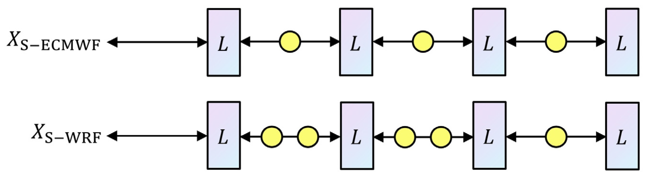
4.2.2. Reversed Sequence Enhancement

Traditionally, data enhancement increases the amount of data to improve the model performance. For oversampling, learning rules from a sparse number of >30 mm data points and generated data similar to actual situations were not easier than the prediction task owing to the complexity of our data. Moreover, there was a greater probability of data overfitting. For undersampling, separating the 0–30 mm data was difficult.

Assuming that meteorological thermodynamics is a reversible process, the display of the reverse process aids in model learning [43]. This is especially the case for the increase in and attenuation of rainfall, as they are important characteristics that affect short-term intensive events. The experiments revealed that, after reverse sequence enhancement, the proportion of each classification was almost invariable; but, the results improved, as shown in

Table 6. Data processing to demonstrate the effectiveness of reversed sequence enhancement. The improvement with the S-ECMWF dataset was more significant than that with the S-WRF dataset. The symbol ‘—’ indicates that the model did not function owing to excessive number of parameters.

Methods	S-ECMWF Predict of First Frame						S-WRF Predict of First Frame
	CSI1	ETS1	FAR1	CSI2	ETS2	FAR2	CSI1	ETS1	FAR1	CSI2	ETS2	FAR2
ASTGCN	0.157	0.074	0.841	0.0114	0.0105	0.9787	0.146	0.052	0.851	0.0004	0.0004	0.9374
ASTGCN + reverse	0.166	0.085	0.830	0.0153	0.0147	0.9714	—	—	—	—	—	—
HDGN	0.115	0.026	0.885	0.0211	0.0202	0.9576	0.134	0.037	0.865	0.0343	0.0336	0.9219
HDGN + reverse	0.123	0.035	0.877	0.0254	0.0252	0.9442	0.152	0.060	0.845	0.0401	0.0395	0.9457

. This provides another means of improving the forecasting accuracy: data should be available to input more valuable information into the model, thereby reducing the difficulty associated with model learning.

However, the reversed sequence enhancement method doubles the amount of data, which almost doubles the training time and increases the space cost of the model. Therefore, there is a trade-off between effectiveness and cost.

4.2.3. Low-Rainfall Sequence Removal

Before training, we removed a portion of the training samples with the least number of data points characterized by non-zero rainfall in the historical sequence. The results in

Table 7. Ablation experiment investigating the effect of low-rainfall sequence removal on the performance of the HDGN model.

Settings	Data Proportion		S-ECMWF Predict of First Frame
	1–30 mm	>30 mm	CSI1	ETS1	CSI2	ETS2
del 0%	0.1240	0.001399	0.113	0.024	0.0204	0.0196
del 5%	0.1239	0.001398	0.118	0.030	0.0202	0.0195
del 10%	0.1281	0.001544	0.115	0.026	0.0211	0.0202
del 15%	0.1246	0.001511	0.115	0.026	0.0202	0.0194
del 20%	0.1241	0.001495	0.115	0.027	0.0199	0.0191
del 50%	0.1196	0.001423	0.117	0.029	0.0179	0.0173

indicate that, owing to the complexity of the rainfall data, this type of elimination could not fundamentally change the imbalance in the data; however, it still improved the prediction performance for short-term intensive rainfall forecasting.

For type 2 indicators, the HDGN model achieved the highest performance when 10% of the data were removed; moreover, the proportion of the >30 mm data points was the highest. Above 10%, the negative effect of the simultaneous decrease in the proportion and volume of the >30 mm data points was observed, which led to underfitting of the model and a reduced model learning ability. Significant performance degradation occurred when the removal ratio exceeded 20%.

For type 1 indicators, the correlation between the removal ratio and indicators was low. Both the proportion and number of the 1–30 mm data points were significantly higher than those of the >30 mm data points; hence, the effect of removing 10% of the data points was relatively smaller. However, it exceeded the effect of not removing data points.

4.2.4. Ablation Study of HDGN

We conducted ablation experiments to analyze the optimal means of designing the HDGN architecture. From

Table 8. Ablation experiments conducted on two datasets to examine the relationship between the number of layers and prediction effect of the HDGN model.

Settings	S-ECMWF Predict of First Frame			S-WRF Predict of First Frame
	CSI2	ETS2	FAR2	CSI2	ETS2	FAR2
4 layers	0.0211	0.0209	0.9576	0.0343	0.0341	0.9219
3 layers	0.0186	0.0181	0.9631	0.0237	0.0229	0.9390
2 layers	0.0007	0.0000	0.9976	0.0016	0.0011	0.9809
1 layer	0.0000	0.0000	1.0000	0.0000	0.0000	1.0000

, the use of a greater number of layers yielded enhanced performance benefits, which aided in the extraction of the correlations between the data. However, this benefit was marginal and restricted by the complexity of the model. Although the spatial size of the high-level feature space was smaller, it corresponded to a larger number of hidden features. The use of a greater number of layers increased the model’s time and space costs. Therefore, we selected a suitable value that yielded satisfactory prediction effects at a low cost.

Another issue was the degree of influence of each dynamic building block on the final result of the HDGN. We compared several schemes under the same premise used for the other configurations, whose results are shown in

Table 9. Influence of the configuration of each dynamic building block on the forecasting results of the HDGN model.

Settings	S-ECMWF Predict of First Frame			S-WRF Predict of First Frame
	CSI2	ETS2	FAR2	CSI2	ETS2	FAR2
HDGN	0.0211	0.0209	0.9576	0.0343	0.0341	0.9219
w/o multiplier	0.0205	0.0203	0.9573	0.0088	0.0082	0.9647
w/o dynamic graphs	0.0000	0.0000	1.0000	0.0000	0.0000	1.0000

, where the w/o multiplier denotes the case where the actual distances between the node pairs were used as the weights of the graphs, while the w/o dynamic graphs denote the case where the dynamic graph generation process was replaced with the supplied fixed graphs. The experimental results showed that the dynamic graph construction scheme was effective. The semantic weights slightly improved the results, whereas removing the entire dynamic graph pooling, including the semantic weights, resulted in serious performance anomalies. Similar to the HDGN model with one layer, their CSI₂ and ETS₂ are smaller than 5 × 10⁻⁵. Significant overfitting of the HDGN model was observed because of the higher decrease in modeling ability than in model complexity in the case where modules were removed. We argue that, in this case, the model can be considered as one that does not have a relevant predictive capability.

5. Conclusions

In this study, we aimed to improve the prediction performance of a short-term intensive rainfall prediction model. To achieve this goal, we described the short-term intensive rainfall prediction task as a spatial–temporal sequence prediction problem and then proposed a non-grid spatial–temporal sequence prediction model, HDGN, which can optimally extract the potential correlations between meteorological data and obtain more accurate prediction results. It consists of three modules: hierarchical graph generation, which is responsible for dynamically generating graphs for multi-level representation of the data from the historical sequences; graph convolution operator generation, which generates the graph convolution operators corresponding to these graphs; and hierarchical graph convolution network, which performs hierarchical feature space extraction and fusion based on the results of the first two modules, followed by frame-by-frame short-term intensive rainfall prediction. The design of the HDGN draws on relevant experience in the field of sequence prediction. To further improve the prediction performance, we also proposed two data enhancement methods for spatial–temporal sequences, namely, reversed sequence enhancement and low-rainfall sequence removal. They are relatively simple to implement, and the training effect is optimized by adding or removing training samples strategically.

The proposed method involves interpolation of rainfall, feature selection for NWP, construction of sequence datasets, data augmentation (optional), training of the HDGN model, and, finally, prediction using the trained model. Compared with the baselines, which included several sequence prediction methods based on deep learning, the experimental results obtained with real-world data from Fujian Province showed that our proposed method significantly improves the short-term intensive rainfall forecasting performance beyond that achieved with pure NWP simulations. On the first prediction frame of the S-ECMWF and S-WRF datasets, CSI2 improved by 9.55 and 6.30 times, and ETS2 improved by 10.22 and 8.08 times, respectively, compared with those of ECMWF and WRF. This method also outperforms the graph-based spatial–temporal sequence prediction model ASTGCN, with improvements of 85.09% and 92.38% in CSI2 and ETS2, respectively, on the first prediction frame of S-ECMWF. On S-WRF, ASTGCN cannot make predictions because of the large size of the graph, whereas HDGN can. Additionally, the proposed reversed sequence enhancement and low-rainfall sequence removal further improved the performance of the HDGN.

The HDGN has the following advantages: (1) It treats different features equally across time and space; thus, the data do not require additional processing. (2) The model’s structure can be adjusted to adapt to different dataset sizes. (3) The prediction speed of the model is high after training.

However, our proposed method has some disadvantages: (1) The HDGN has difficulties when modeling the meteorological evolution at sub-grid and inter-frame scales, characterized by poor predictions for margin regions. (2) Additional measures are needed to further reduce the relatively high FAR of our model. (3) The cost-effectiveness of the reversed sequence enhancement is low.

Owing to this issue, there is much work needed before achieving an ideal short-term intensive rainfall prediction model. Future research should focus on the following aspects: (1) achieve learnable data fusion based on the nature of graphs to avoid errors introduced by the interpolation process; and (2) enhance the modeling capability and response to special regions without losing the generalization ability by combining, for example, the meteorological physical rules.

References

1. Xie, H.; Wu, L.; Xie, W.; Lin, Q.; Liu, M.; Lin, Y. Improving ECMWF short-term intensive rainfall forecasts using generative adversarial nets and deep belief networks. Atmos. Res. 2021, 249, 105281. [Google Scholar] [CrossRef]
2. Liu, C.; Sun, J.; Yang, X.; Jin, S.; Fu, S. Evaluation of ECMWF precipitation predictions in China during 2015–2018. Weather Forecast. 2021, 36, 1043–1060. [Google Scholar] [CrossRef]
3. Wang, T.; Liu, Y.; Dong, C.; Li, J. A summary of research on short-term precipitation forecast method and its application. Electron. World 2019, 41, 11–13. [Google Scholar] [CrossRef]
4. Woo, W.; Wong, W. Operational Application of Optical Flow Techniques to Radar-Based Rainfall Nowcasting. Atmosphere 2017, 8, 48. [Google Scholar] [CrossRef] [Green Version]
5. Huang, X.; He, L.; Zhao, H.; Wu, Y.; Huang, Y. Long-Term intelligent calculation and prediction model for heavy precipitation satellite cloud Images. In Proceedings of the 2018 4th International Conference on Advances in Energy Resources and Environment Engineering, ICAESEE 2018, Chengdu, China, 7–9 December 2018. [Google Scholar]
6. Shi, E.; Li, Q.; Gu, D.; Zhao, Z. A Method of Weather Radar Echo Extrapolation Based on Convolutional Neural Networks. In Proceedings of the 24th International Conference on MultiMedia Modeling, MMM 2018, Bangkok, Thailand, 5–7 February 2018; pp. 16–28. [Google Scholar]
7. Bouget, V.; Béréziat, D.; Brajard, J.; Charantonis, A.; Filoche, A. Fusion of Rain Radar Images and Wind Forecasts in a Deep Learning Model Applied to Rain Nowcasting. Remote Sens. 2021, 13, 246. [Google Scholar] [CrossRef]
8. Boukabara, S.-A.; Krasnopolsky, V.; Stewart, J.Q.; Maddy, E.S.; Shahroudi, N.; Hoffman, R.N. Leveraging modern artificial intelligence for remote sensing and NWP: Benefits and challenges. Bull. Am. Meteorol. Soc. 2019, 100, ES473–ES491. [Google Scholar] [CrossRef]
9. Zhou, K.; Zheng, Y.; Li, B.; Dong, W.; Zhang, X. Forecasting different types of convective weather: A deep learning approach. J. Meteorol. Res. 2019, 33, 797–809. [Google Scholar] [CrossRef]
10. Qian, Z.; Zhou, Q.; Liu, L.; Feng, G. A preliminary study on the characteristics of quiet time and intrinsic dynamic mechanism of precipitation events in the rainy season in eastern China. Acta Meteorol. Sin. 2020, 78, 914. [Google Scholar] [CrossRef]
11. Yin, S.; Ren, H. Performance verification of medium-range forecasting by T639, ECMWF and Japan models from September to November 2017. Meteorogical Mon. 2018, 44, 326–333. [Google Scholar]
12. Yang, Q.; Dai, Q.; Han, D.; Chen, Y.; Zhang, S. Sensitivity analysis of raindrop size distribution parameterizations in WRF rainfall simulation. Atmos. Res. 2019, 228, 1–13. [Google Scholar] [CrossRef]
13. Zhuo, S.; Zhang, J.; Yang, X.; Zi, L.; Qiu, H. Study on Comparison and Evaluation Index of Quantitative Rainfall Forecast Accuracy. J. Water Resour. Res. 2017, 6, 557–567. [Google Scholar] [CrossRef]
14. Chen, M.; Yu, X.; Tan, X.; Wang, Y. A brief review on the development of nowcasting for convective storms. J. Appl. Meteorol. Sci. 2004, 15, 754–766. [Google Scholar]
15. Hochreiter, S.; Schmidhuber, J. Long short-term memory. Neural Comput. 1997, 9, 1735–1780. [Google Scholar] [CrossRef] [PubMed]
16. Narejo, S.; Jawaid, M.M.; Talpur, S.; Baloch, R.; Pasero, E.G.A. Multi-step rainfall forecasting using deep learning approach. PeerJ Comput. Sci. 2021, 7, 1–23. [Google Scholar] [CrossRef]
17. Shi, X.; Yeung, D.-Y. Machine learning for spatiotemporal sequence forecasting: A survey. arXiv 2018, arXiv:1808.06865. [Google Scholar]
18. Liu, Y.; Racah, E.; Correa, J.; Khosrowshahi, A.; Lavers, D.; Kunkel, K.; Wehner, M.; Collins, W. Application of deep convolutional neural networks for detecting extreme weather in climate datasets. arXiv 2016, arXiv:1605.01156. [Google Scholar]
19. Agrawal, S.; Barrington, L.; Bromberg, C.; Burge, J.; Gazen, C.; Hickey, J. Machine learning for precipitation nowcasting from radar images. arXiv 2019, arXiv:1912.12132. [Google Scholar]
20. Zhang, C.; Wang, H.; Zeng, J.; Ma, L.; Guan, L. Tiny-RainNet: A deep convolutional neural network with bi-directional long short-term memory model for short-term rainfall prediction. Meteorol. Appl. 2020, 27, e1956. [Google Scholar] [CrossRef]
21. Shi, X.; Chen, Z.; Wang, H.; Yeung, D.-Y.; Wong, W.-K.; Woo, W.-C. Convolutional LSTM network: A machine learning approach for precipitation nowcasting. In Proceedings of the 29th Annual Conference on Neural Information Processing Systems, NIPS 2015, Montreal, QC, Canada, 7–12 December 2015; pp. 802–810. [Google Scholar]
22. Ji, S.; Xu, W.; Yang, M.; Yu, K. 3D Convolutional neural networks for human action recognition. IEEE Trans. Pattern Anal. Mach. Intell. 2013, 35, 221–231. [Google Scholar] [CrossRef] [Green Version]
23. Sutskever, I.; Vinyals, O.; Le, Q.V. Sequence to sequence learning with neural networks. In Proceedings of the Advances in Neural Information Processing Systems, Montreal, QC, Canada, 8–13 December 2014; pp. 3104–3112. [Google Scholar]
24. Guen, V.L.; Thome, N. Disentangling physical dynamics from unknown factors for unsupervised video prediction. In Proceedings of the IEEE/CVF Conference on Computer Vision and Pattern Recognition, Seattle, WA, USA, 13–19 June 2020; pp. 11474–11484. [Google Scholar]
25. Lan, M.; Ning, S.; Li, Y.; Chen, Q.; Chen, X.; Han, X.; Cui, S. From single to multiple: Leveraging multi-level prediction spaces for video forecasting. arXiv 2021, arXiv:2107.10068. [Google Scholar]
26. Su, J.; Byeon, W.; Kossaifi, J.; Huang, F.; Kautz, J.; Anandkumar, A. Convolutional tensor-train LSTM for spatio-temporal learning. In Proceedings of the 34th Conference on Neural Information Processing Systems, NeurIPS 2020, Virtual, Online, 6–12 December 2020. [Google Scholar]
27. Seo, S.; Liu, Y. Differentiable physics-informed graph networks. arXiv arXiv:1902.02950, 2019.
28. Wang, X.; Ma, Y.; Wang, Y.; Jin, W.; Wang, X.; Tang, J.; Jia, C.; Yu, J. Traffic flow prediction via spatial temporal graph neural network. In Proceedings of the Web Conference 2020, Taipei, Taiwan, 20–24 April 2020; pp. 1082–1092. [Google Scholar]
29. Zheng, C.; Fan, X.; Wang, C.; Qi, J. Gman: A graph multi-attention network for traffic prediction. In Proceedings of the AAAI Conference on Artificial Intelligence, New York, NY, USA, 7–12 February 2020; pp. 1234–1241. [Google Scholar]
30. Guo, S.; Lin, Y.; Feng, N.; Song, C.; Wan, H. Attention based spatial-temporal graph convolutional networks for traffic flow forecasting. In Proceedings of the AAAI Conference on Artificial Intelligence, Honolulu, HI, USA, 27 January–1 February 2019; pp. 922–929. [Google Scholar]
31. Fang, Z.; Long, Q.; Song, G.; Xie, K. Spatial-temporal graph ODE networks for traffic flow forecasting. In Proceedings of the 27th ACM SIGKDD Conference on Knowledge Discovery & Data Mining, Singapore, 14–18 August 2021; pp. 364–373. [Google Scholar]
32. Qi, Y.; Li, Q.; Karimian, H.; Liu, D. A hybrid model for spatiotemporal forecasting of PM2.5 based on graph convolutional neural network and long short-term memory. Sci. Total Environ. 2019, 664, 1–10. [Google Scholar] [CrossRef] [PubMed]
33. Li, F.; Feng, J.; Yan, H.; Jin, G.; Jin, D.; Li, Y. Dynamic graph convolutional recurrent network for traffic prediction: Benchmark and solution. arXiv 2021, arXiv:2104.14917. [Google Scholar]
34. Lin, X.; Liu, A.; Lin, Y.; Xu, J. Technical Manual of Weather Forecast of Fujian Province; China Meteorological Press: Beijing, China, 2013. [Google Scholar]
35. Xie, H.; Zhang, S.; Hou, S.; Zheng, X. Comparison research on rainfall interpolation methods for small sample areas. Res. Soil Water Conserv. 2018, 25, 117–121. [Google Scholar]
36. Fu, B.; Peng, M.S.; Li, T.; Stevens, D.E. Developing versus nondeveloping disturbances for tropical cyclone formation. Part II: Western North Pacific. Mon. Weather Rev. 2012, 140, 1067–1080. [Google Scholar] [CrossRef] [Green Version]
37. Diehl, F. Edge contraction pooling for graph neural networks. arXiv 2019, arXiv:1905.10990. [Google Scholar]
38. Henaff, M.; Bruna, J.; LeCun, Y. Deep convolutional networks on graph-structured data. arXiv 2015, arXiv:1506.05163. [Google Scholar]
39. Simonovsky, M.; Komodakis, N. Dynamic edge-conditioned filters in convolutional neural networks on graphs. In Proceedings of the IEEE Conference on Computer Vision and Pattern Recognition, Honolulu, HI, USA, 21–26 July 2017; pp. 3693–3702. [Google Scholar]
40. Kipf, T.N.; Welling, M. Semi-supervised classification with graph convolutional networks. In Proceedings of the 5th International Conference on Learning Representations, ICLR 2017, Toulon, France, 24–26 April 2017. [Google Scholar]
41. He, K.; Zhang, X.; Ren, S.; Sun, J. Deep residual learning for image recognition. In Proceedings of the 29th IEEE Conference on Computer Vision and Pattern Recognition, CVPR 2016, Las Vegas, NV, USA, 26 June–1 July 2016; pp. 770–778. [Google Scholar]
42. Paszke, A.; Gross, S.; Massa, F.; Lerer, A.; Bradbury, J.; Chanan, G.; Killeen, T.; Lin, Z.; Gimelshein, N.; Antiga, L. Pytorch: An imperative style, high-performance deep learning library. Adv. Neural Inf. Processing Syst. 2019, 32, 8024–8035. [Google Scholar]
43. Foresti, L.; Sideris, I.V.; Nerini, D.; Beusch, L.; Germann, U. Using a 10-year radar archive for nowcasting precipitation growth and decay: A probabilistic machine learning approach. Weather Forecast. 2019, 34, 1547–1569. [Google Scholar] [CrossRef]
Figure 1. Distribution of each ground station in Fujian Province. The colors indicate the total number of observed short-term intensive rainfall events in February 2015 to December 2018 for each station [1].
Atmosphere 13 00703 g001
Figure 2. The overall architecture of the proposed Hierarchical Dynamic Graph Network (HDGN) model. It consists of three main modules: hierarchical graph generation, graph convolution operator generation, and Hierarchical Graph Convolutional Network (HGCN). The model is dynamic in nature because it uses different graphs for different sequences.
Atmosphere 13 00703 g002
Figure 3. Hierarchical graph generation process generates high-level graphs G l ( l > 0 ) from initial graph G 0 , historical sequence, and geographic distance between nodes (NodeDist).
Atmosphere 13 00703 g003
Figure 4. Proposed hierarchical graph convolutional network as the sequence prediction part of HDGN. Schematic shows the detailed structure of a three-layer network, where circles are components and rectangles are data. A rectangle’s bottom area and height characterize the size of graph and feature space, respectively.
Atmosphere 13 00703 g004
Figure 5. Hierarchical graph convolutional networks adapted to S-ECMWF or S-WRF datasets, where boxes represent one layer, circles represent graph data pooling and de-pooling operations.
Atmosphere 13 00703 g005