1. Introduction
Recent developments in machine learning (ML) and artificial intelligence (AI) techniques have a great deal of influence on broad applications, such as autonomous vehicles, medical services, stock price prediction, military weapons, and home appliances. People generally want to use AI techniques to solve or improve the problems that they face. However, the choice of ML techniques along with the preparation of training sets often creates new problems that they have never experienced. In particular, the optimizing performance of ML results based on various experiments takes a long time. Accordingly, the optimization work is considered to be technical tuning rather than scientific. These ML trends are far from the AI technology that people want for scientific achievement. This technical demand has led to the development of automatic AI technology to recommend the best ML technique or automatically optimize hyperparameters [
1,
2,
3,
4,
5,
6].
For neural network (NN) training, it is important to optimize the selection of hyperparameters related to training conditions, such as the number of neurons and hidden layers, activation functions, batch sizes, learning rates, and epochs. This is because the optimized hyperparameters are largely dependent on the characteristics of the training sets. This study focuses on Sherpa developed in Hertel et al. (2020) [
2]. The dictionary definition of Sherpa is a person hired to guide mountain climbers in the Himalayas. Sherpa provides the robust optimization of hyperparameters in NN training, such as batch normalization (yes or no), dropout, activation functions, learning rates, and the numbers of neurons and hidden layers. Although it was only recently released, the automatic optimization of Sherpa is widely used for various topics, such as sub-grid parameterization in climate modeling [
7,
8], the development of the Fortran–Keras Bridge software [
9], Raman spectroscopy [
10], particle physics [
11], electron identification [
12], prediction of wave height [
13], prosthetic vision [
14], pulmonary coccidioidomycosis [
15], petrophysical rock [
16], mixed script identification [
17], and surge prediction in coastal areas [
18]. Using Sherpa, the variability of hyperparameters in the NN can be reduced by up to 90% while maintaining prediction accuracy [
19].
This study focuses on the application of Sherpa in developing radiation emulators based on the NN. Many emulation studies are performed on radiative transfer processes and their applications in numerical climate/weather prediction models. Emulation studies for radiative transfer processes are conducted using various ML techniques, such as the feed-forward NN [
20,
21,
22,
23,
24,
25], convolutional neural network [
20], adaptive network-based fuzzy inference systems [
22], recurrent neural network [
25], classification and regression tree and random forest [
26], and U-net++ model [
27]. However, most emulation studies for numerical prediction models are based on the use of NN because of the difficulties associated with numerical prediction models [
26,
28,
29,
30,
31,
32,
33,
34,
35,
36,
37,
38,
39,
40]. Because these studies aim at a significant speedup of numerical prediction models using radiation emulators, deep network models with heavy computation cannot be considered.
In this study, the Sherpa results were applied to the radiation emulator for the Weather Research and Forecasting (WRF) model [
41] developed by Song et al. (2022) [
38]. This emulator showed a 60-fold speed improvement for the radiation process and an 87% reduction in the total computation time required for the WRF simulation. This study is concerned with how automatic optimization by Sherpa can be beneficial to improving the accuracy of numerical weather forecasting. Because optimization attempts for previous radiation emulators were performed relying on manual sensitivity experiments, this study can significantly contribute to achieving maximum accuracy without cumbersome experiments. We also want to verify that Sherpa’s optimization can exhibit a universal performance even in long-term predictions that are linked to the WRF model. Among the utility of Sherpa, discrete choices, such as batch normalization and activation functions, are not very helpful in optimizing NN training because they are possible through individual experiments without Sherpa. The dropout is difficult to apply a numerical prediction model based on Fortran. Neurons and hidden layers are important parameters that determine the accuracy and computational cost of the radiation emulator. However, if we consider a fixed computational cost, the number of neurons and hidden layers should not be changed to fairly compare the resultant accuracy. Finally, the learning rate with a continuous range is the most appropriate hyperparameter for testing the Sherpa performance. Along with this experiment, this study also considered the batch sizes used in batch normalization. The impact of these hyperparameters on improving weather forecasting accuracy is discussed in this study.
2. Data and Methods
This study considered the training datasets used in Song et al. (2022) [
38] to develop a radiation emulator imitating the RRTMG-K radiation parameterization [
42]. The training sets were generated for the period 2009–2019 in Korea. Although it consisted of 96 categories (longwave (LW)-shortwave (SW), clear-cloud, land-ocean, and 12 months), only the July period was used in this study. More specifically, the training sets were sub-sampled by combining four days for 2009–2018 and the July period of 2019 with an even weighting (i.e., 50% for the 4 days and 50% for 2019). The four days in the training sets consisted of two days for the first and second maximum heavy precipitation events that occurred in the July period of 2009–2018, along with randomly sampled non-precipitating two days. The validation sets consisted of another 2 days for the third and fourth maximum heavy precipitation events that occurred in July 2009–2018, along with 2 non-precipitating days not used in the training sets. Each set comprised 3 million cases with 193 inputs (158 for clear) and 42 outputs. The input variables were pressure, air temperature, water vapor, ozone, and cloud fraction profiles, in addition to surface variables, such as skin temperature, surface emissivity, insolation, and surface albedo. The output variables were the atmospheric heating rate profiles and upward/downward fluxes at the top and bottom, excluding the downward component at the top. Note that the number of vertical profiles used was 39 layers.
In NN training, the use of stochastic weight averaging (SWA), developed by Izmailov et al. (2018) [
43], is known to express the strength in generalization. This study also applied SWA for the last 25% of epochs. The number of epochs for NN training was determined by Song et al. (2022) [
38] as being 3000 and 2200 for clear and cloud cases, respectively. The max min normalization and standard normalization were used for the inputs and outputs, respectively. The numbers of neurons and hidden layers were fixed at 90 and 1, respectively, to maintain a 60-fold speedup compared to the original radiation parameterization. Considering the numerical complexity [
32,
38], the computational speed of the emulator is inversely proportional to the numbers of neurons and hidden layers. The hyperbolic tangent was used as the activation function. By examining 15 activation functions by Song et al. (2022) [
38], the hyperbolic tangent was determined to be the most appropriate function for this topic.
Control simulations (L1 and L2) were performed by applying two learning rates with the lowest and highest values (0.0001 and 1) for different batch sizes (3,000,000: full, 50,000, 5000, and 500). Here, the batch size indicates the size of the training data separated for parallel (or batch) learning. When the learning rate was less than 0.0001, the results no longer changed significantly; thus, the lowest value was set as 0.0001. Note that Song et al. (2022) [
38] used a batch size of 500 and a learning rate of 0.05 through empirical experiments. However, because infinite experiments on batch sizes and learning rates are impossible, automatic optimization using Sherpa is necessary. The Sherpa experiments were conducted in the range of 0.0001–1 for learning rates, along with discrete batch sizes (full, 50,000, 5000, and 500). Thus, the optimized learning rate for a given batch size was determined using Sherpa. Sherpa provides several algorithm functions to optimize hyperparameters [
2]. Among various optimization algorithms, the genetic algorithm was selected for this study. In a previous study [
44], the genetic algorithm exhibited better results than random search and grid search algorithms in terms of spatial distribution search and computational speed, respectively, for Canadian Institute For Advanced Research 10 classes (CIFAR-10) image datasets. The use of the random search algorithm in this study exhibited a similar result within the 0.5% range for training loss compared with the genetic algorithm. Although the use of more trials can give further optimization, the computation time for training is proportional to the number of trials. The number of trials was empirically set to three, resulting in the Sherpa experiments taking 3-fold more training time compared with one control simulation, consuming approximately 1 day under the NVIDIA DGX A100 graphics processing unit (GPU). If GPU resources are sufficient, more trials can be attempted for further development. Nevertheless, the use of Sherpa still has an advantage in terms of computation time because infinite testing of the learning rates is impossible.
The control simulations (L1 and L2) and Sherpa results were finally stored in the form of weight and bias coefficients (from inputs to the hidden layer, as well as a hidden layer to outputs). Using these coefficients, offline testing was performed on independent validation sets that were not used in the training sets. The number of datasets (3,000,000 × 8) and the structure of the inputs and outputs for the validation sets were the same as those for the training sets. In the offline testing, the land and ocean results were averaged by considering a fractional land area of 45.30% in an environment where training sets were generated. The clear and cloud results were simply averaged. The 42 output variables were separated into 39 heating rate profiles and three fluxes. The two categories were mainly analyzed while naming the LW/SW heating rates and LW/SW fluxes. In the online testing, the weight and bias coefficients were implemented in the WRF model in the form of a radiation emulator. A total of 28 days in July 2020 were simulated with a 20 s time step over 234 × 282 horizontal grids. The radiation emulator was used approximately 8 billion times temporally and spatially. Thus, the datasets used in the online prediction were 333-fold bigger than 24 million training data. It can be regarded as a challenging task in machine learning fields. This study will mainly analyze the long-term forecast accuracies for LW/SW fluxes, skin temperature, and precipitation when radiation emulators based on two control simulations (L1 and L2) and Sherpa were applied to the WRF model.
3. Results
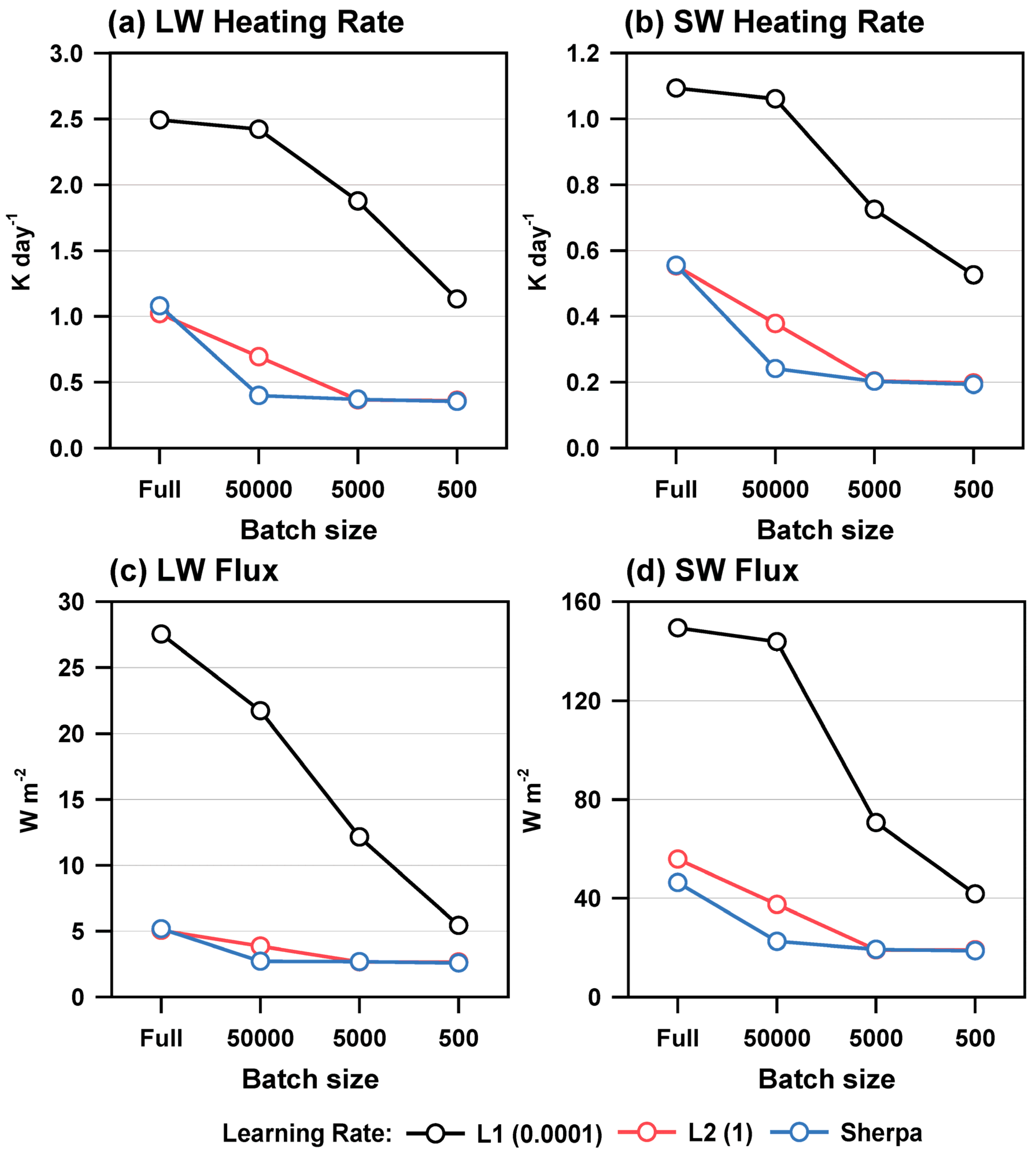
Figure 1 show the RMSE of LW/SW heating rates and LW/SW fluxes between the control simulations (L1 and L2) and Sherpa experiments for the offline evaluation (i.e., for independent validation sets). Here, the land and ocean results are combined, and all sky conditions, including clear and cloud conditions, are considered. In the Sherpa experiment, the optimal learning rates were determined to be 0.6199, 0.6032, 0.6656, and 0.4756 for batch sizes of full, 50,000, 5000, and 500, respectively. These results are thought to be related to the argument that batch size and learning rate should be proportionally used to obtain a consistent result [
45]. The Sherpa also exhibited the lowest optimal learning rate (0.4756) for the smallest batch size. The optimal learning rates by Sherpa were closer to L2 (1) than L1 (0.0001). We suspect the possibility of affecting a large number of training sets on these systematic optimal learning rates to L2. However, before conducting experiments on learning rates, we could not recognize the optimal learning rate because it is highly sensitive to the characteristics of the training sets. Therefore, Sherpa can help determine an optimal learning rate without extensive sensitivity experiments. In
Figure 1, it is evident that the RMSEs tend to decrease for small batch sizes. The use of an appropriate small batch size is generally known to provide better accuracy than the full batch size [
46]. Nevertheless, the use of small batch size is not popular compared to the full batch for attempting because of the increase in computation time owing to less parallelization. The L1 experiments show a dramatic error decrease with decreasing batch size, whereas the L2 experiment represents a gradual error decrease. Thus, the difference between L1 and L2 decreased as the batch size decreased. This is because the error in the L1 experiment is too large when the batch sizes are large. For the L2 experiments, there was no significant difference in batch sizes of 5000–500, suggesting that there is an optimal range of batch sizes for a given problem. The Sherpa experiments showed evidently smaller RMSEs than L1 for all variables. This confirms the usefulness of Sherpa in automatically optimizing the learning rate. However, for the full batch, the difference between L2 and Sherpa was not large. The RMSEs for the LW/SW heating rate and LW flux were slightly larger in the Sherpa experiment than in L2. Because the optimization of Sherpa was performed on the training set, robust generalization may not be sufficient for independent validation sets (this issue also continues in the online testing). The difference between L2 and Sherpa was the largest at a batch size of 50,000, and this difference was almost diminished for batch sizes of 5000–500. Thus, it can be understood because the optimal learning rates inferred by Sherpa are close to the L2. In conclusion, Sherpa contributed to the RMSE improvements of 131–507%, 97–339%, 111–701%, and 123–539% for LW heating rate, SW heating rate, LW flux, and SW flux, respectively, compared with the L1 experiment. When compared to the L2 experiment, the maximum RMSE improvements by Sherpa were 74%, 57%, 42%, and 66% for the four variables at a batch size of 50,000, while significant further improvements were not found for different batch sizes, except for SW flux at the full batch size (20%).
It is also of note that the results in
Figure 1 were based on all sky conditions, including clear and cloud conditions. Considering only the clear areas, the RMSEs tended to decrease significantly (
Figure 2). The overall trends shown in
Figure 2 are similar to those shown in
Figure 1. Based on the Sherpa experiment, the RMSEs of LW heating rate, SW heating rate, LW flux, and SW flux for the all sky condition were 2.51–7.79, 2.21–12.02, 2.83–4.79, and 2.73–16.07 times larger than those for clear, respectively. These results suggest that this study deals with a challenging problem for all sky conditions, which is more difficult than other studies for cloud-free conditions [
20,
21,
23,
25]. Thus, this leads to interest in the next results when the radiation emulator is applied to a complex weather forecasting model.
Figure 3 show the spatial distributions of outgoing LW radiation (OLR) simulated from radiation emulators trained with different batch sizes (full to 500) and learning rates (L1, L2, and Sherpa) for an extreme precipitation case associated with the Changma front (2020-07-28/03UTC). This case was long-term integrated with 156 h forecasts initialized from 2020-07-21/15UTC. Because a 20 s time step and 65,988 spatial grids were used, the radiation emulator was repeatedly used in the WRF model 1,852,943,040 times (28,080 × 65,988). Physically, OLR is highly sensitive to the presence of clouds. If there is a cloud, the OLR tends to decrease because a colder temperature, compared with the surface, is emitted from the cloud top. Thus, in
Figure 3, red colors indicate clear areas, whereas green, blue, and purple represent clouds. In particular, purple areas with the lowest OLR indicate deep convective clouds. When the full batch size and lowest learning rate were used (
Figure 3a), the simulated OLR pattern was far from the true value based on the original radiation parameterization (
Figure 3m). The OLRs in
Figure 3a are mostly distributed around 200 and 300 W m
−2. This simulation is a typical blow-up case induced by the use of an incorrect radiation emulator. Belochitski and Krasnopolsky (2021) [
35] also produced unphysical OLRs when the developed radiation emulator had a large representation error when online testing was significantly different from training sets. For a batch size of 50,000 and the lowest learning rate (
Figure 3d), the blow-up issue appeared to be somewhat mitigated but not completely solved. For example, deep convective clouds with an OLR of approximately 100 W m
−2 were not expressed at all in
Figure 3d. When the batch sizes were further decreased to 5000–500 (
Figure 3g,j), the OLR simulations also tended to be close to the true value. When the highest learning rate was used, the simulated OLRs for all batch sizes showed a reliable pattern with the true value, whereas further improvements were found with the use of small batch sizes (
Figure 3b,e,h,k). The Sherpa experiments also showed similar OLR patterns to the true values (
Figure 3c,f,i,l). When the batch sizes were large, Sherpa was thought to be more useful compared with the two control simulations.
For a more quantitative analysis, the time series of the RMSE for the LW flux, SW flux, and skin temperature was further examined (
Figure 4). Note that the flux results are the average of the three fluxes at the top and bottom of the atmosphere. In
Figure 4, 168 forecast time results were given at a 3 h resolution. Each point in the time series indicates the statistics for the four weekly cases with different initializations and for the entire domain (234 × 282 grids). When the full batch size was used, the RMSEs of the simulated LW/SW fluxes and skin temperature fluctuated within the range of larger values. Compared to the lowest learning rate, the results of the highest learning rate and Sherpa showed lower RMSEs for the three variables (
Figure 4a–c). A similar trend was also observed for the case using a batch size of 50,000 (
Figure 4d–f). When the batch size decreased, the differences among the emulator results also tended to decrease (
Figure 4g–l). In both full and 50,000 batch sizes, the Sherpa results were evidently better than the highest learning rate results. In contrast, the two emulators did not show much difference for batch sizes of 5000 and 500, although they were still better than the lowest learning rate. The resulting RMSEs for LW/SW fluxes and skin temperature tended to gradually increase with forecast time while showing a diurnal fluctuation between day and night. The increase in isolation and surface heating during the daytime are thought to affect the diurnal fluctuation.
Figure 5 display the spatial distributions of the LW flux error for the use of different batch sizes (full to 500) and learning rates (L1: 0.0001, L2: 1) in the control simulations, as well as Sherpa. The RMSE value in each grid denotes a statistical value for 28 days with 3 h intervals. For the full batch size, the forecast errors of the LW flux were much larger than those for the smaller batch sizes. The largest RMSEs were observed in the L1 experiment for the full batch size. Large forecast errors were mostly distributed over high-altitude regions, such as northwest China and North Korea, including the Baekdusan Mountain. This can be understood by the difference in altitudes between land and ocean because the surface temperature and associated LW flux are highly correlated with topography. In addition, the L1 experiment with the lowest learning rates produced the largest error among the three experiments (L1, L2, and Sherpa) for all batch sizes. This problem in the L1 experiment was somewhat mitigated for a batch size of 500. The L2 experiments showed characteristically lower errors for batch sizes from full to 5000 compared to the L1 experiments. The Sherpa experiments showed a much smaller error than the L1 and L2 experiments. In particular, the difference between the Sherpa and control simulations (L1 and L2) was large for large batch sizes. Note the full batch learning was most actively used in NN training as a default setting. Therefore, Sherpa will be very useful for finding the optimal approximation in NN training. However, for small batch sizes [
46] or sequential training [
47], the optimization of Sherpa on the learning rate is not very helpful for improving the performance of NN training. Similar results for different batch sizes and learning rates were also found for the SW flux and skin temperature (
Figure 6 and
Figure 7). For the SW flux, there was no evident contrast between land and ocean, unlike the LW flux (
Figure 5), because surface emissivity and temperature were not input variables for the SW radiation process.
The difference between the Sherpa and L2 experiments was not evident in the offline evaluation for the validation sets because it was not connected to the WRF model (
Figure 1). In contrast, we can also see a huge difference between the Sherpa and L2 experiments, as well as between the Sherpa and L1 experiments in
Figure 4,
Figure 5,
Figure 6 and
Figure 7. This is because the results shown in
Figure 4,
Figure 5,
Figure 6 and
Figure 7 were obtained by repeatedly using the radiation emulator within the WRF model (i.e., online prediction). A more quantitative analysis is found in
Table 1, which show the total statistics for all temporal periods and the entire domain. The statistics were derived from 224 3 h intervals (28 days) and 65,988 grids.
Table 1 present the RMSEs for LW flux, SW flux, skin temperature, and precipitation. At the full batch size, Sherpa contributed to improvements of 39–125%, 81–92%, 137–159%, and 24–26% for the four variables compared with the L1/L2 experiments. The error improvements for precipitation were the smallest among the four variables because it is an output indirectly affected by the radiation emulator. As shown in
Figure 1, the difference between the Sherpa and L2 experiments was negligible at the full batch size, except for the SW flux, which showed a 20% improvement. In contrast, the Sherpa results in
Table 1 show 39% and 81% improvements for the LW and SW fluxes, respectively, compared with the L2 experiment based on full batch size. The contrast can be understood by the difference between the offline (
Figure 1) and online tests (
Table 1) associated with the link to the WRF model. It also suggests that the forecast accuracy in the online test is not guaranteed, even if it is satisfied with sufficient accuracy in the offline test. At a batch size of 50,000, similar improvements for Sherpa were maintained at 37–140%, 61–124%, 95–198%, and 17–33% for the four variables. However, for the batch size of 5000, the error improvements by the use of Sherpa were found when compared with the L1 experiment, such as 74%, 42%, 50%, and 16% for LW flux, SW flux, skin temperature, and precipitation, respectively. These improvements were further reduced by 26%, 20%, 25%, and 13% for the batch size of 500. In conclusion, these results suggest that the use of Sherpa for optimizing the learning rate can be powerful when the batch size is large in developing a radiation emulator for a weather prediction model.
4. Summary and Conclusions
This study investigated the usefulness of Sherpa in optimizing learning rates for developing a radiation emulator based on a feed-forward NN. The evaluation of the radiation emulators using Sherpa, along with two control simulations based on the lowest and highest learning rates (L1: 0.0001 and L2: 1), was performed under two frameworks: offline and online evaluations. For each experiment, four batch sizes (full, 50,000, 5000, and 500) were considered. The offline evaluation was for 24 million cases independent of the training sets, whereas the online evaluation was conducted under the WRF simulations for the July 2020 period over the Korean peninsula by using weight and bias coefficients from the NN. In offline testing, all experiments showed an evident error reduction with decreasing batch size in predicting the LW/SW heating rates and fluxes. The L2 experiment exhibited a much smaller error than L1, whereas the Sherpa result showed a similar or better accuracy compared with L2. Sherpa contributed to improvements of 131–507%, 97–339%, 111–701%, and 123–539% for LW heating rate, SW heating rate, LW flux, and SW flux, respectively, compared with the L1 experiment. The improvements achieved by Sherpa were significant when the batch sizes were larger than 50,000. In the online evaluation, the radiation emulator was used approximately 8 billion times spatially and temporally, in contrast to a one-time application in the offline evaluation. The L1 results for batch sizes of full to 50,000 produced unphysical OLRs because of the lower accuracy of the radiation emulators developed under these configurations. At the full batch size, Sherpa contributed to reducing the forecast errors for LW flux, SW flux, skin temperature, and precipitation by 39–125%, 81–92%, 137–159%, and 24–26%, respectively, compared with the two control simulations. These improvements were further reduced by 26%, 20%, 25%, and 13%, respectively, for a batch size of 500 compared with the L1 experiment. The usefulness of Sherpa was clearly displayed in the time series and spatial distributions for the forecast errors of LW/SW fluxes and skin temperature. Overall, the Sherpa results were similar to those of the L2 experiment using the highest learning rate (1), in contrast to L1, using the lowest learning rate (0.0001). This was because the optimal learning rates inferred from Sherpa were 0.4756–0.6656, which is similar to 1. It is also of note that the radiation emulator based on Sherpa at the full batch also exhibited significant improvements of 26–137% in predicting LW/SW fluxes, skin temperature, and precipitation in the online testing, in contrast to a negligible improvement compared with the L2 experiment in the offline testing.
Although similar performance without the help of Sherpa can be achieved through various sensitivity experiments, Sherpa has a valuable advantage in automatically optimizing hyperparameters (learning rate in this study). The advantage can be powerful in the case of big data, where various sensitivity experiments require too many computational resources, such as in the development of radiation emulators in numerical weather forecasting models. The Sherpa is thought to provide a universally applicable optimal solution by lowering the representation error even if it is applied to very different conditions from the trained situation. This benefit is important for developing a universal radiation emulator for operational weather forecasting because all data in nature cannot be fully covered regardless of how training sets are used, while the emulator should be applied to the operational model that predicts the future in real-time. In conclusion, the active use of Sherpa can be useful to maximize the performance of the radiation emulator in the numerical weather prediction model.


