Particle Sedimentation in Numerical Modelling: A Case Study from the Puyehue-Cordón Caulle 2011 Eruption with the PLUME-MoM/HYSPLIT Models

Abstract

Numerical modelling of tephra fallout is a fast-developing research area in volcanology. Several models are currently available both to forecast the dispersion of volcanic particles in the atmosphere and to calculate the particles deposited at different locations on the ground. Data from these simulations can then be used both to manage volcanic crises (e.g., protect air traffic) or perform long-term hazard assessment studies (e.g., through hazard maps). Given the importance of these tasks, it is important that each model is thoroughly tested in order to assess advantages and limitations, and to provide useful information for quantifying the model uncertainty. In this study we tested the coupled PLUME-MoM/HYSPLIT models by applying them to the Puyehue–Cordon Caulle 2011 sub-Plinian eruption. More specifically, we tested new features recently introduced in these well-established models (ash aggregation, external water addition, and settling velocity models), we implemented a new inversion procedure, and we performed a parametric analysis. Our main results reaffirm the pivotal role played by mass eruption rate on the final deposit and show that some choices for the input parameters of the model can lead to the large overestimation in total deposited mass (which can be reduced with our inversion procedure). The parametric analysis suggests a most likely value of the mass eruption rate in the range 2.0–6.3 × 10⁶ kg/s. More studies with a similar approach would be advisable in order to provide final users with useful indications about the parameters that should be carefully evaluated before being used as input for this kind of model.

1. Introduction

Numerical modelling of tephra transport, dispersion, and sedimentation has become a key research area in volcanology e.g., [1,2,3,4,5,6]. On the one hand, numerical models are important to better understand and describe the physics of particle sedimentation, e.g., [7,8] or particle aggregation, e.g., [5,9], but also of larger scale phenomena such as ash cloud development [10] or effects of variable source parameters on transport [11]. On the other hand, numerical models are invaluable tools during volcanic crisis for rapid forecasts of volcanic clouds by the different Volcanic Ash Advisory Centers, or VAACs, Refs. [12,13,14] but also for developing long-term probabilistic maps related to tephra fallout [15,16,17,18,19]. However, these two latter tasks could be accomplished if, for the employed models, there is a good balance between a physically reliable reproduction of the phenomena and acceptable computational times (see [20] for a review) that, especially for operational purposes, is on the order of several minutes to few hours [21]. The nine VAACs that operate worldwide currently use six different tephra transport and dispersal models for real-time tracking of volcanic particles [22], each of them initialized with different source conditions and meteorological data [23]. The same models are also widely used in the production of tephra fallout probabilistic hazard maps. Regarding the source conditions (i.e., the spatio-temporal release of particles/mass from the eruption column to the volcanic cloud), they could range from simple geometric distributions to 1D integral models [2] and 3D models [24], while complex multicomponent and multiphase flow models are still too expensive from a computational point of view [20]. Meteorological data (typically wind field, air density/temperature, and, in some cases, humidity, pressure, boundary layer altitude, turbulence, and precipitation) are necessary to simulate the transport of tephra cloud. These can be forecast models [25,26] or reanalysis of global meteorological models [27,28,29], usually stored as 4D meteorological datasets.

As discussed by Ref. [20], significant improvements in the modelling of tephra transport, dispersal, and sedimentation have been put forward over the past years, such as: (a) the implementation of satellite data assimilation techniques to improve the real-time particle tracking; (b) the use of ensemble probabilistic forecasts to account for eruptive source parameters uncertainty; or (c) the improvement of the computational efficiency of numerical models to reduce computational times. Nevertheless, several mechanisms that can highly influence tephra transport, dispersal, and sedimentation are still poorly considered or neglected in the models used operationally and in hazard-related studies. For instance, particle aggregation [30,31,32] has been implemented only sporadically in numerical models, e.g., [33,34,35], while other broader scale, en masse depositional mechanisms such as ash fingering [36,37,38] or sediment waves [39] have not been included in any model to date. Moreover, the employment of different meteorological datasets with different spatio-temporal resolutions and different atmospheric parameters could lead to great differences in simulation outputs, even if the source conditions are the same [40].

Numerical models have become a crucial tool for managing the tephra hazard in real time and understanding related processes [20]. Still, it is necessary to acknowledge the above-mentioned limitations, study their impact on the results, and identify potential areas of improvement. A commonly used and effective strategy for this is to evaluate the models by reproducing a past eruption for which there are sufficient and reliable field measurements including uncertainties (plume heights, total mass of deposit, deposit thickness at some location, duration, or meteorological data) and by validating the approach in two possible ways: either by demonstrating that the model is internally consistent and without known flaws [5,40,41,42,43,44,45,46,47,48] or by quantifying the overall uncertainty in model outputs from the forward propagation of parameter uncertainties [40,47,49,50].

In this paper, we therefore test the current capabilities of coupling an integral plume model (PLUME-MoM) with a Lagrangian particle transport model used for tephra dispersal (HYSPLIT); the latter is currently used by three VAACs [22] for operational purposes, while in this study the former is used to provide the source conditions for HYSPLIT. The two models have been also used recently by Ref. [51] to develop tephra fallout hazard maps. Given its large application in such critical fields, new developments of the models need to be tested rapidly. Particular emphasis is therefore devoted to analyzing the effects of modelling features recently incorporated in PLUME-MoM [33] but whose contribution has not yet been tested on particle sedimentation from HYSPLIT, such as wet/dry aggregation, addition of external water at the vent, and different settling velocity models (this latter feature has also been included in HYSPLIT in this study). Moreover: (i) we implement a procedure to invert observations (i.e., mass loading at specific locations and average plume height) in order to better characterize eruptive source parameters; and (ii) we perform a parametric analysis on the main input parameters of the two models in order to assess the relative contributions of each of them in influencing particle sedimentation. The test case is the well-studied 2011 Puyehue-Cordón Caulle (Chile) sub-Plinian eruption [52].

The paper is organized as follows. Section 2 reviews the test eruption and the two models. Section 3 presents the methods, including our comparative approach, the inversion procedure, and the parametric analysis. Finally, we present results, discussion, and conclusions in Section 4, Section 5 and Section 6, respectively.

2. Background

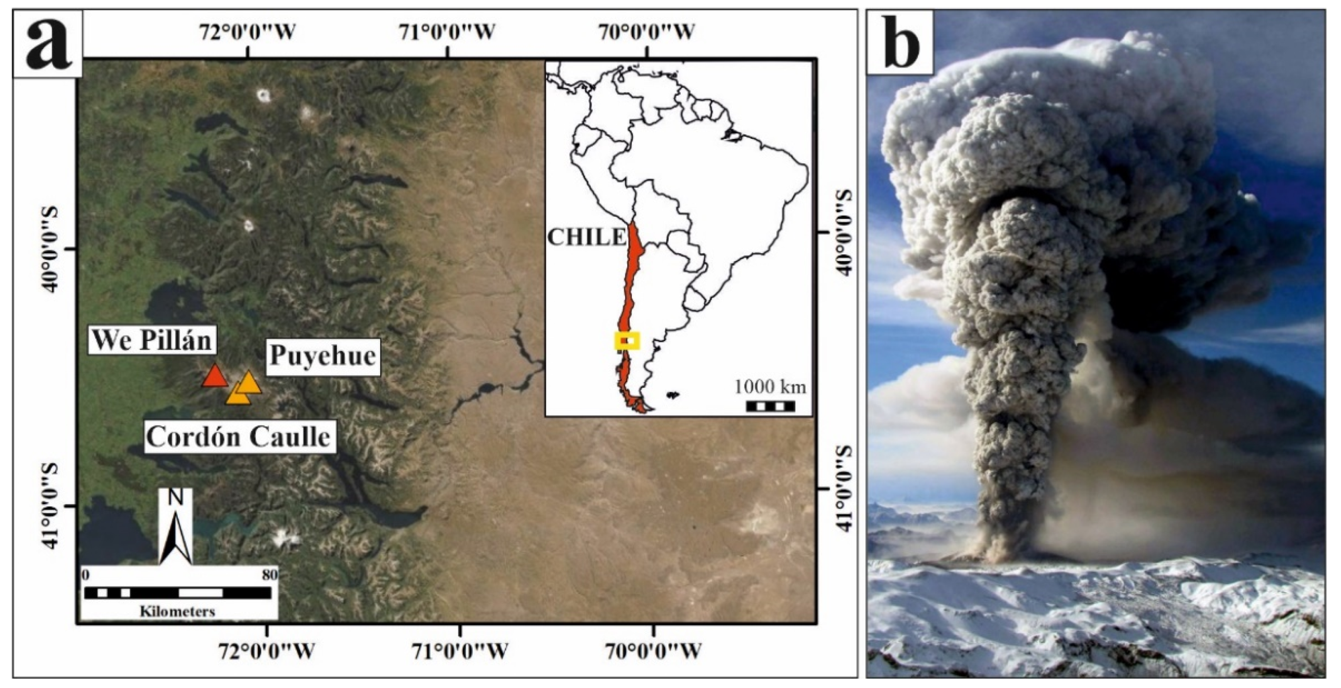
2.1. The 2011 Puyehue-Cordón Caulle Eruption

The Puyehue-Cordón Caulle 2011 eruption (PCC11- Figure 1) started on 4 June at 14:45 LT (18:45 UTC), and involved the formation of a new vent 7 km NNW from the main crater of the Puyehue-Cordón Caulle complex (“We Pillàn” vent-Figure 1a; [52]).

This eruption involved magma of rhyolitic-rhyodacitic composition [53], lasted until June 2012 [54], and comprised both explosive and effusive activity [55]. The latter resulted in the emission of ~0.5 km³ of rhyodacitic lava [54]. The main explosive phase (Unit I, layers A-F; [56]) lasted approximately 17–27 h between 4–5 June [54,57] and featured: (i) a plume height varying between 9 and 12 km above vent [52,57]; (ii) an average mass eruption rate (MER) of 7.3 × 10⁶ kg/s [57]; and (iii) a total erupted mass of 4.5 ± 1.0 × 10¹¹ kg [56]. With these values, this eruption was classified as sub-Plinian with a VEI of 3–4 by [57]. Finally, Ref. [53] calculated the total grain size distribution (TGSD) of Unit I in the range −4Φ/11Φ, using different datasets and methods (i.e., Voronoi tessellation, weighted average of samples, and mass of individual Φ sizes). Globally, main results indicated that: (a) TGSD has a bimodal distribution with the two sub-populations (with modes at −2Φ and 7Φ) separated by the 3Φ grain size; (b) the fine subpopulation is associated with size-selective sedimentation processes (e.g., particle aggregation, convective instabilities); and (c) grain size bimodality is related to a significant lack of particles in the 3Φ size.

This eruption has been the focus of multiple studies which compared the observed and modelled values of: (a) column height [40]; (b) column mass load (i.e., the integration of the mass of the ash cloud along the atmospheric vertical levels; [51,58]); and (c) ground deposit measurements (thickness and mass loading, [52,59]); mass loading and grain sizes [40].

2.2. The PLUME-MoM/HYSPLIT Model

For this work, we used the integral plume model PLUME-MoM and the particle transport and dispersion model HYSPLIT, as already performed by Refs. [4,40], coupled through a suite of Python scripts (see “Data Availability Statement”). First of all, the column model is initialized with a meteorological profile extracted at the vent location by HYSPLIT from the meteorological datasets. Then, the mass lost from the plume edges at intervals of fixed height and that reaching the neutral buoyancy level are processed to define the source locations and rates for HYSPLIT.

In this paper, we use a newly released version of PLUME-MoM (PLUME-MoM-TSM, [33]). As in the first version of Ref. [60], PLUME-MoM solves the equations for the conservation of mass, momentum, energy of the gas-particle mixture, and for the conservation of mass of the individual phases (solid particles and gas components). The model accounts for particle loss during the plume rise and for radial and crosswind air entrainment parameterized using two entrainment coefficients, and adopts the method of moments to describe a continuous size distribution of one or more group of particles (i.e., juveniles, lithics, aggregates, etc.). New features introduced by Ref. [33] for PLUME-MoM-TSM include:

• The simulation of particle aggregation according either to the wet aggregation model proposed by Ref. [9] or to a constant “dry” aggregation kernel (see Appendix A for details);
• The possibility to add external water at the vent or incorporated through ingestion of moist atmospheric air, and the phase transition of water (vapor, liquid, or ice) according with the pressure-temperature conditions. By adding external water, magma-water mixing takes place at the vent, thermal equilibrium is reached, and PLUME-MoM updates magma temperature and water phases partitions before their interaction with the atmosphere;
• The possibility to simulate the spreading of the umbrella cloud intruding from the volcanic column into the atmosphere, with a transient shallow water system of equations which models the umbrella cloud as an intrusive gravity current affected by the wind;
• The possibility to model particle settling velocity with three different schemes, i.e., those of Ganser [61], Textor [62], and Pfeiffer [63] (see Appendix B for details);
• The possibility to model the presence of additional volcanic gases such as CO₂ and SO₂ (transported as passive components).

Apart from the last point, all the other features have been tested in this work due to our focus on particle sedimentation. In the following sections, we will use PLUME-MoM and PLUME-MoM-TSM as synonyms.

The HYSPLIT model [64] belongs to the family of Lagrangian transport and dispersion models, and solves the Lagrangian motion equations for the horizontal transport of pollutants (volcanic particles in our case), while vertical motion depends on the pollutant terminal fall velocity. The dispersion of a pollutant is described using three main types of configuration, “3D particle”, “puff”, or hybrid “particle/puff”. Particularly in the “puff” configuration, mass is partitioned into packets of ash particles (“puffs”) having a horizontal gaussian distribution of mass described by a standard deviation σ. The puffs expand with atmospheric turbulence until they exceed the size of the meteorological grid cell (either horizontally or vertically) and then split into several new puffs, each with their respective mass. For our simulations, we used the hybrid “particle/puff” configuration, that is a circular 2D object (planar mass, having zero vertical thickness), in which the horizontal pollutant has a “puff” distribution and in the vertical is treated as a particle; this configuration allows us to use a limited number of puffs to properly capture both the horizontal dispersion and the vertical wind shears [40]. In this work we have used the April 2018 release version of HYSPLIT, with the modifications detailed in Ref. [40] and summarized in Appendix C. Finally, we added the settling velocity models of Textor and Pfeiffer [62,63], in addition to that of Ganser [60] originally included in HYSPLIT, in order to provide uniformity with those used in PLUME-MoM-TSM (point iv of the paragraph about PLUME-MoM).

3. Methods

3.1. Comparison Parameters

In order to evaluate the effect of the most important features of the model on particle sedimentation, we used several data from the literature related to the Unit I, Layers A-F of the PCC11 eruption (see Section 2) and a specific approach. In particular (Figure 2), we used: (i) mass loading (in kg/m²) measured at 75 sampling points, (ii) grain size values (MdΦ, the median of the grain size distribution measured in the Krumbein Φ scale) measured at 24 sampling points [56], along with (iii) isomass lines (in kg/m²) reported in Ref. [53]. In addition, we also considered (iv) 13 reconstructed test sites located along the main dispersal axis of the PCC11 eruption provided by Ref. [40] using the GDAS meteorological data. These latter sites are used to evaluate the along-axis differences in particle sedimentation throughout the different model configurations, that is, without aggregation (both with and without the addition of external water), with the “wet” aggregation model of Ref. [9] and with a constant “dry” aggregation model. We underline that, with respect to the addition of external water and also the “wet” aggregation model, we are testing such configurations just to explore the model current capabilities, as the eruption does not present any phreatomagmatic signature cf. [53,56,57]. We also remind readers that, presently, aggregation is modeled only within PLUME-MoM, not within HYSPLIT. Consequently, the newly formed aggregates are treated by HYSPLIT as single particles with a specific diameter (and density) and it is not possible to “disaggregate” them once they settle. Thus, the deposits used for the comparisons are composed of both non-aggregated particles and aggregates treated as single particles. As the proportions between the two are not available, we are only evaluating the differences in grain size for each site, not the mass loading. It is important to observe that aggregation depends on the particle-particle interactions, and thus on their volumetric fraction within the volcanic column and cloud. While at lower levels in the column the solid fraction is large enough to favor aggregation, higher in the column and in the cloud this is less likely, and thus modeling aggregation only within the column represent a good approximation of the real phenomenon.

The along-axis reconstructed test sites are also used to define transects orthogonal to the dispersal axis (Figure 2), which are in turn the basis to estimate the total mass deposited within such transects, both from field data and from simulations. To do so, within a GIS environment we used the isomass lines (both those from field data and those produced after the simulations) converted into polygons, whose areas are multiplied by the value of the isomass line itself.

We also tested 4 different meteorological datasets (

Table 1. List of meteorological files used in this study.

Name	Type	Atmospheric Parameters	Pressure Levels	Spatial Resolution	Temporal Resolution
ERA-Interim	Reanalysis	10	37	1° (~100 km)	6 h
NCEP/NCAR	Reanalysis	11	17	2.5° (~250 km)	6 h
GDAS	Forecast	35	23	1° (~100 km)	3 h
ERA5	Reanalysis	10	37	0.28° (~31 km)	1 h

): (1) the ERA-Interim [27] and (2) the ERA5 reanalysis data [28], both elaborated by the European Centre for Medium-Range Weather Forecasts (ECMWF); (3) the NCEP/NCAR Global Reanalysis Data [29] and (4) the Global Data Assimilation System (GDAS) archive [26], both developed by the National Oceanic and Atmospheric Administration (NOAA). The main differences within the different datasets are summarized in Table 1, and are related to their typology (forecast/reanalysis), the atmospheric parameters/pressure levels (i.e., the vertical subdivisions) and the spatio-temporal resolution of the dataset.

3.2. Inversion Procedure

We have implemented an inversion procedure in order to find the best combination of PLUME-MoM/HYSPLIT inputs that minimize the differences between modeled and observed outputs. Given that we are using a coupled plume and dispersal/sedimentation model, we considered plume height (final output of PLUME-MoM) and ground mass loading (final output of HYSPLIT) as the parameters to fit in order to minimize the difference between simulated and observed values. The best-fitting inverse procedure for this coupled model was aimed, following Ref. [65], at minimizing the T² function, which has been modified in the following form

$$T_{Total}^2=T_{PH}{}^2+T_{ML}{}^2={\displaystyle \sum }_{i=1}^{N_{PH}}{\left[\frac{P{H}_{o,i}-P{H}_{m,i}}{P{H}_{o,i}}\right]}^2+{\displaystyle \sum }_{i=1}^{N_{ML}}{\left[\frac{M{L}_{o,i}-M{L}_{m,i}}{M{L}_{o,i}}\right]}^2$$

(1)

where T_PH² and T_ML² are the T² functions calculated using plume height (in m above vent) and mass load (in kg/m²), respectively, and PH_o,I and ML_o,i denote the observed plume height and the observed mass load, respectively, while PH_m,i and ML_m,i are the corresponding values predicted by the model. $N_{PH}$ and $N_{ML}$ are, respectively, the 75 sampling points used in the inversion (Figure 2) and the two average daily measurements (corresponding to the two days of the main explosive phase, see Section 2.1) of plume height provided by Ref. [53], which have been compared with two daily averages of plume heights values provided by PLUME-MoM.

The parameters for which the inversion was performed and their range of variation are reported in

Table 2. List of parameters considered for the simulations in the inversion procedure (Inv-NA and Inv-NAProx; see Table 3 and Section 4.3) and in the parametric analysis (S-Dak; see Table 3). The parameters which control diffusion (K_mixd, K_mix0, K_zmix, K_def, K_bls, and K_blt) are detailed in Appendix D.

Parameter	Description	Used in PLUME-MOM (PM) or HYSPLIT (HY)	Unit	Continuous (C) or Discrete (D)	Type	Lower Value	Upper Value
MER	Mass eruption rate of particles transported in plume	PM	kg/s	C	-	105.5	107
Water mass fraction	Water mass fraction of the magma	PM	wt%	C	-	4	7
At-vent velocity	Initial exit velocity from the vent	PM	m/s	C	-	135	275
Tmix0	Initial temperature of the erupted mixture	PM	K	C	-	1073	1273
ρ1	Particle density assigned to Φ = −4	PM	kg/m3	C	-	500	1000
ρ2	Particle density assigned to Φ = 5	PM	kg/m3	C	-	2500	2670
Cp	Particle heat capacity	PM	J/(kg × K)	C	-	1100	1600
SF	Particle shape factor	PM/HY	-	C	-	0.6	0.7
Settling velocity	Settling velocity model considered	PM/HY	m/s	D	Ganser	-	-
					Textor
					Pfeiffer
Meteorological file	Meteorological dataset considered	PM/HY	-	D	GDAS	-	-
					NCEP/NCAR
					ERA-Interim
					ERA5
Kmix0	Minimum mixing depth	HY	m	D	Every 100 m	100	500
Kzmix	Vertical Mixing Profile	HY	-	D	Varies with height	-	-
					Single average value
Kdef	Horizontal Turbulence	HY	-	D	Proportional to vertical turbulence	-	-
					From velocity deformation
Kbls	Boundary Layer Stability	HY	-	D	Heat/momentum flux	-	-
					Wind/temperature profile
Kblt	Vertical Turbulence	HY	-	D	Beljaars/Holstag	-	-
					Kantha/Clayson
					Velocity variance

. Two types of parameters are considered: “continuous” and “discrete”. The former have been sampled at each iteration from a continuous distribution between two extremes (lower value and upper value) while the latter have been sampled from a discrete number of values/options. Among all the parameters, seven of them (mass eruption rate, water mass fraction, vent velocity, initial temperature, densities of coarse-fine particles, and particle heat capacity) are used only by PLUME-MoM, five of them (K_mixd, K_mix0, K_zmix, K_def, K_bls, and K_blt) are used only by HYSPLIT to control diffusion processes, and the remaining are used by both models.

3.3. Parametric Analysis

In this paper, we have also performed a parametric analysis with respect to the parameters listed in Table 2. This approach was aimed at assessing the contribution of each parameter in the definition of the total variability in the T² function, as similarly investigated in Ref. [49]. In our approach, however, due to the presence of discrete variables (settling velocity, meteorological files, and the parameters that control turbulence in HYSPLIT), we have instead analyzed correlation plots of two discrete variables (settling velocity model and meteorological files) and eight continuous variables (initial water content, mass eruption rate, exit velocity, initial temperature, initial/final values of the density profile of the particles, heat capacity, and particle shape factor). The parameters that control diffusion in HYSPLIT (see Appendix D) have been analyzed separately in a similar correlation plot. This distinction has been made in order to separately evaluate the effects on T² of the parameters that control particle/eruption characterization and those controlling atmospheric characterization.

4. Results

In the following sub-sections we present the simulations performed, summarized in

Table 3. List of simulations performed in this study.

Simulation(s) Code	N° Simulations	Aggregation	External Water	Settling Velocity Model	Other Parameters
NA	1	No	No	Ganser	Table S1
NAEW	1	No	Yes	Ganser	Table S1
AD	1	Yes (dry)	No	Ganser	Table S1
AW	1	Yes (wet)	Yes	Ganser	Table S1
NAP	1	No	No	Pfeiffer	Table S1
NAT	1	No	No	Textor	Table S1
Inv-NA	250	No	No	All	Table 2
Inv-NAProx	250	No	No	All	Table 2
S-Dak	900	No	No	All	Table 2

. Additional information on the parameters used can be found in Table 2 and in Table S1 from the Supplementary Material. The same total grain size distribution has been used for all the simulations, calculated by Ref. [53] and listed in Table S1 from the Supplementary Material.

4.1. Effect of Initial Water and Dry/Wet Aggregation

We performed four types of simulations (Table 3) in PLUME-MoM, respectively:

• no aggregation (“NA”);
• no aggregation but with the addition of 10 wt% (weight %) of external water (“NAEW”);
• with the dry aggregation model with a constant aggregation kernel β = 10⁻¹⁵ m³/s (“AD”). This value is consistent with that used in Ref. [33];
• the aggregation model of Ref. [9], considering the addition of 10 wt% of external water (“AW”).

The newly formed aggregates are considered as a different group of particles with respect to parent ones, with different densities and different shape factors with respect to the parent particles. The values for aggregates density and shape factor have been derived from Ref. [66].

For the simulations, we have used the same set of parameters as in Ref. [40]: the GDAS meteorological dataset (Table 1 from this study) and the Ganser settling velocity model (see Appendix B). In particular, the latter two have been chosen because: (a) the GDAS dataset is one of the two released by NOAA (along with the NCEP/NCAR Reanalysis, see Table 1) that could be employed in HYSPLIT without format conversion (as necessary for ERA-Interim and ERA5, see Table 1), and the one among the two with a better reproduction of past eruptions (see [40]); (b) the Ganser settling velocity model [61] is one of the default models used in HYSPLIT and the only one originally present in both models. The complete list of parameters used for such simulations is available in Table S1 from the Supporting Information.

We show in Figure 3 the along-axis differences (every 10 km) in grain size distribution for the four simulation types. For all the simulations, we can observe in the deposit a shift of median Φ size toward fine classes with increasing distance from vent. The grain size graphs also show that the differences between the “NA” and the “NAEW” simulations are not particularly marked for all the test sites up to 120 km. Contrastingly, with the occurrence of whichever type of aggregation process (dry or wet), markedly coarser particles are formed early at the expense of finer ones beyond 10 km in range. The difference among simulations including aggregation (“AD” and “AW”, respectively) is mostly revealed at ranges of 20–60 km from the vent by a coarser median of the particle size distribution during dry aggregation (–4 to –3 with dry aggregation and –3 to –2 with wet aggregation). To better quantify the effect of aggregation, we also show in Figure 3 an aggregation index (Δmm), measuring the effect of aggregation on the median value of the grain size distribution. Δmm represents the difference in the median of the deposit grain size (converted from the Φ scale to mm) between the simulations with aggregation and without aggregation. The higher the value of Δmm, the greater the difference in grain size due to the effect of aggregation. Positive Δmm indicates a shift toward larger median clasts with aggregation. We have calculated Δmm for both the “dry” (“AD”-“NA”) and “wet” (“AW”-“NAEW”) conditions.

The strong control of aggregation on sedimentation is revealed by striking differences in the grain size distributions (GSDs) of simulated deposits, for both dry and wet eruptive conditions, between conditions of aggregation versus without aggregation. In particular, departures in GSD modes and median values, although relatively weak up to 20 km, increase considerably thereafter as seen from the Φ-scale values and also from the quantified aggregation index in mm (Figure 3 inset). Differences in median value between aggregation and no aggregation cases (for both wet and dry conditions) are around 2 mm at ultra-proximal sites (0–10 km), peak at ~12–13 mm at 30–40 km from the vent, and then drop regularly down to the same value of ~2 mm at 80 km. Despite the fact that similar absolute values of the aggregation index (2 mm) are observed at ultra-proximal (0–10 km) and distal sites (>90 km), note that, proportionally, the increase in median grain size under the effect of aggregation is greater at more distal sites, for instance ~0.5 mm without aggregation versus ~2.5 mm with aggregation at 0–10 km, and ~10 mm without aggregation versus ~12 mm with aggregation at >90 km.

4.2. Effect of Different Settling Velocity Models

In addition to the simulations presented in the previous section, we performed three further simulations in which we have considered (in both PLUME-MoM and HYSPLIT) the three settling velocity models detailed in this study (Ganser, Pfeiffer, and Textor; see Appendix B). For such simulations (named NA, NAP, and NAT, respectively-see Table 3) we have not considered aggregation and we have used the same set of parameters as Table S1 and the GDAS meteorological dataset (Table 1) for the same reasons specified in Section 4.1. We have compared the simulated values with those deriving from field data of: (1) the total mass deposited in each transects defined in Section 3.1 (Figure 4a–d); (2) the mass loading values at the sampling points of Ref. [56], according to the classic approach used to validate similar numerical models, e.g., [67,68] (Figure 4e).

In Figure 4d, the modelled data provide a total mass value which is, on average, three times greater than the total mass obtained considering the mass loading isolines from field data. This latter (0.95 × 10¹¹ kg) represents only a fraction of the total mass measured for the eruptive phase (4.5 ± 1.0 × 10¹¹ kg; see Section 2.1). With respect to the different transects, up to 80 km from the vent (87% of the total mass from field data), the total mass of the simulations are 2–5 times larger than those observed, while the situation is the opposite beyond 80 km. We note that beyond 80 km from the vent, the number of sampling points close to the axis is much lower than at <80 km. Differences among the total mass obtained with the three settling models are lower than 8%. Among the simulations performed with the three settling velocity models, the one performed using the Ganser model shows a peak of mass accumulation in the 30–40 km transect, while those performed using Textor and Pfeiffer have their peaks in the 20–30 km transect. The simulation performed using Pfeiffer has total mass values within the highest peaks that are intermediate between the Ganser and the Textor ones. If considered as a whole, however, differences in total mass among the three settling velocity models are of second order importance compared to the differences with field data.

Concerning the comparison with the mass loading at the sampling points of Ref. [56] (Figure 4e), for the three settling models (Ganser, Pfeiffer, and Textor), the percentage of sampling points within 5 times and 1/5 of the observed value are very similar (67%, 68%, and 65%, respectively). We recall that having a good amount of sampling points that fall within 5 times and 1/5 of the observed values (less than one order of magnitude each way) is considered a proxy for good model/observation correlation (see, e.g., [20]).

The along-axis comparison of grain sizes and mass loadings (Figure 5, every 10 km) shows instead, similarly to Figure 3, that differences among the three simulations are weak up to 20 km with respect to the grain size distribution but are high with respect to mass loading. For instance, at the vent location, the simulations give 400 kg/m² for Ganser, and 800 kg/m² for Textor, with Pfeiffer’s being in between. From 20 km and beyond, compared to the Ganser simulation, Textor and Pfeiffer simulations generally have (a) a grain size distribution shifted toward more fine-grained values; (b) lower mass loading values. Absolute differences in mass loading among the three simulations tend to be negligible beyond 80 km.

4.3. Inversion from Field Data

The inversion procedure has been performed using the procedure described in Section 3.2 considering the simplest case with no aggregation. We have neither considered the aggregation cases nor the addition of external water because for the former it is not possible to recalculate the mass loading with disaggregated particles (and therefore compare it with field data), while for the second this eruption does not show any sign of phreatomagmatism.

As comparable parameters, we have considered (i) the mass loading measured at the 75 sampling points of Ref. [56] and (ii) the two daily averaged plume height values (one per each day of the eruptive phase considered) derived from Ref. [57]. In total, we performed 250 simulations considering all 75 sampling points. Additionally, we performed 250 simulations considering only a subset of the sampling points. The distance of 80 km from the vent divides the deposit in two zones where the total mass deposited by the simulations is, respectively, higher (before 80 km) and lower (beyond 80 km) than the total mass given by field data (see Figure 4). We have therefore considered only the sampling points within 80 km from the vent where most of the tephra mass was deposited (87%) and most of the field data points were collected (56 out of 75). The idea is to verify whether it is possible to obtain a global improvement of the outputs (i.e., the total mass and the mass for each transect, see Section 3.1 and Figure 4) by using a subset of the sampling points that fall within an area of general overestimation of the simulation with respect to field data.

Table 4. Values of the T² minimization function from two simulations (Inv-NA (best) and Inv-NAProx (best)) from the inversion procedure with the lowest T² values. The T² values of the NA simulation (see Section 4.2 and Figure 4c) is reported for comparison. PH and ML subscripts refer to, respectively, the T² values with respect to plume height measurements and mass loading at sampling points, while the subscript TOTAL refers to the sum between the former two.

Simulation Code	T2PH	T2ML	T2Total
NA	41	520	561
Inv-NA (best)	81	167	248
Inv-NAProx (best)	46	122	168

reports the T² values for the best two inversions (i.e., with the lowest T²) for the whole sampling point dataset (Inv-NA) and the subset of sampling points < 80 km (Inv-NAProx). For comparison, we also include the T² values of the NA single simulation of Figure 4c which, among the three cases described in Section 4.2, is the one with the lowest T²_Total value.

For the two simulations with the lowest T² values of Table 3 (whose parameters are listed in Table S2 from the Supplementary Material) we have calculated (Figure 6): (1) the total mass deposited in each transects defined in Section 3.1 (Figure 6a–c); (2) the comparison simulated/observed mass loading values at the 75 sampling points of Ref. [56] for which there is a mass loading measure (Figure 6d); and (3) the comparison simulated/observed median grain size (MdΦ) at the 24 sampling points of Ref. [56] for which there is a grain size analysis (Figure 6e).

The T² values of Table 4 show that the inversion procedure allows us to significantly improve the agreement between simulation results and observations, as shown by the large decrease in T²_Total values (from 561 to 168, see Table 4), especially those related to mass loading (ML). This is also reflected by the lower values of mass for each transects and in total (Figure 6c) as compared to Figure 4d. The total mass overestimation with respect to field data is still by a factor of 2 (2.26 and 1.93 for Inv-NA (best) and Inv-NAProx (best), respectively). Regarding mass loading (Figure 6d), the number of sampling points falling within the limits of a factor 5 of field observations are 68% for the whole dataset (Inv-NA, 75 data points) and as much as 85% for the subset of 56 sampling points within 80 km from the vent (Inv-NAProx).

For the best inversion simulations we have also evaluated the modeled versus observed median values of the grain size distribution (MdΦ) for all the sampling points (Figure 6e), given the better results related to the reproduction of the total mass (Figure 6c). For the best-fitting scenario, for 54% and 67% of the sampling points, respectively, within 120 km (13 out of 24, Inv-NA) and within 80 km (12 out of 18, Inv-NAProx), the simulated median values are comprised within ±1 Φ with respect to those from field observations.

4.4. Parametric Analysis

In addition to the simulations studied for the inversion procedure (see Section 4.3), we performed a total of 900 simulations (S-Dak—see Table 3) to study the sensitivity of mass loading at the 75 sampling sites to the different parameters of Table 2. For this analysis, we have used the open source DAKOTA toolkit [69]. At each iteration, the Latin hypercube sampling method has been adopted to properly cover the parameter space [70]. In this method, the range of each variable is divided into segments of equal probability, and a sample is selected randomly from each of these equal probability partitions. As discussed in Ref. [49], this approach has the advantage that, through the subdivision of the parameter space in equal probability partitions, the samples generated are uniformly distributed over each marginal distribution, and it requires a smaller number of samples than a classical Monte Carlo approach to cover the entire parameter space with the desired accuracy.

The results obtained from this set of simulations are presented with correlation plots (Figure 7 and Figure 8), which are helpful to investigate the dependence between multiple variables at the same time and to highlight the most correlated variables in a data table. In our case, we are investigating the dependency between the T² minimization function and (a) the three settling velocity models and the eight continuous parameters related to particle properties and eruption features (Figure 7a), (b) the four meteorological datasets and the eight continuous parameters related to particle and eruption features (Figure 7b), and (c) the five parameters that control diffusion in HYSPLIT (Figure 8).

From these plots (Figure 7a,b), it can be seen how mass eruption rate exerts a primary control on the T² function, as all outputs line up on a quasi-linear decay trend (from 10^5.5 down to 10^6.3–10^6.8, depending on parameter) followed abruptly by a quasi-vertical increase in the minimization function. This suggests a most likely value of the mass eruption rate in the range 2.0–6.3 × 10⁶ kg/s. This value is comparable but slightly lower than the average estimate of Ref. [57] (see Section 2.1). The simulation outputs of the other parameters (Figure 7) are generally scattered without any obvious trend, therefore indicating that their control on the T² function, if any, is secondary with respect to mass eruption rate.

Regarding instead the two sets of discrete parameters that compose Figure 7 (i.e., settling velocity model and meteorological dataset): (1) the Ganser settling velocity model provides the smallest range of variation of the T²_Total values up to ~4000, while the other two reach similar higher values up to ~8000; (2) the NCEP/NCAR meteorological dataset provides the greatest T²_Total values, while the other three (GDAS, ERA-Interim, and ERA5) have the same range of variation of T²_Total values.

The correlation plots between the T² function and the parameters that control diffusion in HYSPLIT (Figure 8) show instead that all of these parameters provide a very similar range of variations of the T² function.

5. Discussion

5.1. Effect of Initial Water, Dry/Wet Aggregation, and Different Settling Models

In this study, we have performed simulations with an amount of added external water of 10 wt% of the initial erupted mass, a quantity consistent with the simulations performed by Refs. [33,71]. The low differences between GSDs of the NA and NAEW simulations of Figure 3 suggest that the sole addition of external water into the eruptive column, without further trigger of aggregation, does not modify the spatial distribution of particle sizes in the deposits. This is explained because external water is an input parameter for PLUME-MoM, and the main outputs of this model are the plume height and the amount of particles released along the plume, which in turn influence particle transport and deposition. Small variation in particle deposition is therefore caused by small variations of plume height as a result of external water addition; this latter is consistent with Figure C1 from Ref. [33]. In fact, this figure shows the effects on plume dynamics (for PLUME-MoM-TSM) of the addition of different amounts of external water (10, 20, 30, and 40 wt%) for constant mass eruption rates. For 10 wt% of external water and for a mass eruption rate comparable to the ones we used in this study (~10⁷ kg/s), a “wet” plume is 1–2 km lower in elevation with respect to a “dry” plume. This variation in plume height is maintained for all the amounts of external water tested by Ref. [33]. Overall, we can assume that, for a mass flow rate of 10⁷ kg/s, the small variation in plume height due to the addition of different amounts of external water does not alter the dynamics of particle deposition. Indeed, the column remains sustained despite the addition of different amounts of external water. More important differences in the spatial distribution of particles are, however, expected for mass eruption rates > ~10^7.5 kg/s. In Ref. [33] it is in fact shown that, above such a value, a “dry” plume collapses, while “wet” plumes are still sustained up to ~10⁹–10¹⁰ kg/s.

Our tests, performed considering two models of aggregation, confirm that in both cases the final deposits have quite different grain size distributions as compared to simulations without aggregation (see Figure 3). As a general consideration, we observe that, with the chosen atmospheric conditions and the chosen eruptive source parameters (see Table S1 from the Supplementary information), the aggregates are formed mostly for grain sizes > −2 Φ (0.25 mm) and > 0 Φ (1 mm) for the “wet” and the “dry” aggregation models, respectively (see maroon bars in Figure S2 from the Supplementary Information). Consistently, most of the differences in grain size between the aggregation models are concentrated in the sampling points between 20 and 70 km from the vent (see Figure 3), where most of the particles > 0 Φ are deposited. Farther than 70 km, grain size distributions are mostly limited to two bins (see Figure 3) with fewer aggregates, explaining the small differences observed also in the Δmm (inset of Figure 3). The lower amount of aggregates formed in our simulations with the model of Ref. [9] is also explained with the low amount of liquid water available compared to ice (see [33] and Figure S4 from the Supplementary Information), which reduces the sticking efficiency. However, as noted in Section 4.1, farther than 70 km from vent the relative differences between aggregation and no aggregation are proportionally higher than in ultra-proximal sites. This could be linked to the fact that the chosen parameters of the aggregates (density and shape factor, see Table S1 from the Supplementary Information) are considerably different with respect to the non-aggregated particles (in terms of their density and shape factor), and therefore they are able to travel much further thanks to their aerodynamic properties. Therefore, the choice of the parameters of the aggregates is crucial in influencing the final deposits, and should be carefully evaluated. We also remind readers that, presently, (i) the grain sizes calculated by HYSPLIT for the deposit do not “disaggregate” the aggregates according to the amount of parent particles that compose each aggregate and (ii) the calculated GSDs describe the relative proportions of the different grain sizes, but not those absolute values. For these reasons, the total mass loading at each site has not been shown as it is influenced by the density of the aggregates. Our preliminary observations therefore call for new studies, aimed at evaluating the real grain size distribution when aggregation is also accounted by the transport/dispersal model. Field observations are in fact concordant in saying that, once settled, most of the aggregates tend to break down in particles of smaller sizes [30].

On the contrary, mass loading variations have been evaluated with respect to the different settling velocity models tested (see Figure 4). An important parameter that we used for comparing field and modelled data is the total mass deposited within transects drawn along the main dispersal axis. Although several limitations of this approach should be considered (isomass lines used for such calculations are drawn after human or automatic interpolations from a limited amount of data points, for both field data and simulations), the comparison is still interesting to highlight the accuracy of the model in reproducing the observed deposit. In general, for simulations NA, NAP, and NAT where default values from the literature are used (Table S1; [40,53,56,57]), the total deposited mass up to 120 km from the vent is much higher in the simulations compared to observations (Figure 4d). Between the simulations performed with the three settling velocity models (NA, NAP, and NAT) and field data, we observe a difference of a factor of 3, with a slightly better value considering the Textor model. Such large differences between field and modelled data cannot be ignored, and highlight that model calibration and evaluation should also consider this parameter (i.e., total mass deposited) to have a clear understanding of the capabilities and to identify how to improve the model itself. Differences in total mass between model and deposit are especially high between 20 and 60 km from vent. An explanation for such a difference (in addition to human/automatic inaccuracies in isomass drawing) could be linked to the non-consideration (in HYSPLIT) of near-vent sedimentation mechanisms (e.g., sediment waves [39]; two-way coupling effect [7]; and settling-driven gravitational instabilities [72]). In this view, an increase in particle sedimentation in the surrounding of the vent (i.e., up to 1 km, where field data are also possibly underestimated) by considering such phenomena within the model could reduce the amount of particles deposited in the subsequent transects. Calculating the total mass deposited is also an important complement with respect to the comparison of mass loading from sampling sites (Figure 4e and Figure 6d) that are normally considered (see, e.g., [20]). For instance, in our case, the amount of sites within a factor of 5 with respect to the perfect fit line in Figure 4e could indicate that, with the parameters employed, the model works fairly well. However, this conclusion is challenged after deep analysis considering the total deposited mass, and differences could only be reduced with the inversion procedure (see following sections). Among the three models, it is important to highlight that most of the differences along the axis in terms of mass loading (Figure 5) are appreciable up to 70–80 km from vent, while they tend to be negligible in the more distal sites. This latter fact is correlated with the larger differences in settling velocities that the three models have for particles > 0Φ (see Figure S3 from the Supplementary Information) as compared to finer ones. The models of Textor and Pfeiffer provide higher values for settling velocities in general, and markedly for coarser particles, which therefore tend to settle closer to the vent with respect to the simulation using Ganser.

5.2. Inversion

We have used a slightly different formulation of the classic T² function in this paper, for example with respect to Ref. [65]. The availability of plume heights, both as measurements during the eruption and as output values from the model [40], allowed us to overcome the problem linked to the presence of a limit in the increase in the T² function in case of no deposition. This could produce several cases in which, for example, a set of parameters which causes almost no deposition at the sampling sites, gives as output a relatively low T² value, as sampling points could not obviously assume negative values of mass loading.

The results of our inversion are important in terms of minimizing the T² function, especially if compared to the NA simulation (see Table 4): the T² value of this latter is in fact more than two times larger than the best inversion considering all the sampling points (Inv-NA) and more than three times larger than the best inversion considering only proximal points (Inv-NAProx). Mass overestimation of the model in the different transects is now reduced up to two times more than field data, but is still considerable (Figure 6c). In the absence of similar comparison with other models, this discrepancy should be therefore considered if PLUME-MoM/HYSPLIT is used to derive, for instance, hazard maps. Among the inverted parameters, we highlight that for the two simulations with the lowest T² values in Table 4 the corresponding settling velocity model is that of Ganser, while the meteorological datasets are ERA-Interim and ERA5, respectively. The former is consistent with experimental data where the Ganser settling velocity model has been considered a good approximation for real particles (see, for instance, [36]). Regarding the meteorological datasets, ECMWF products (i.e., ERA-Interim and ERA5) appear to provide a better reproduction of the real deposit. However, we note that such datasets are more difficult to be employed in HYSPLIT (due to conversion issues from a different file format) and do not systematically provide the best results for all eruption types (see Section 5.3 and [40,51]). The employment of a subset of sampling site (Inv-NAProx) is also useful to produce an overall improvement of the total mass deposited (see Table 4 and Figure 6c,d). Due to the better reproduction of the total mass deposited, for only these two simulations (Inv-NA and Inv-NAProx) we have also evaluated the difference with respect of field data of the median of the grain sizes (MdΦ, Figure 6e). This parameter is the most difficult to be reproduced by numerical model [40], and in our case there is a slightly better reproduction of the best simulation of the Inv-NAProx set (although there is a lower amount of sampling points). For our simulations, we relied on the TGSD calculated by Ref. [53], as they considered a good amount of single grain size analyses even from ultra-distal sites (being therefore highly representative of the whole deposit). However, future developments could also evaluate whether the overall reproduction of the deposit is improved by also varying the TGSD in the inversion procedure.

5.3. Parametric Analysis

The PLUME-MoM/HYSPLIT coupled models have a quite large number of parameters that could be varied (see Table 2), and it is important to quantify the contribution of each parameter in influencing the final result (in this case the plume height and the total mass deposited, see Section 3.3). In this way it is possible to identify whether or not a parameter could be used with a default value, therefore reducing the complexity of model initialization. In our parametric analysis (see Section 3.3) it is important to highlight some important trends (see Figure 7 and Figure 8). Firstly, it is evident that mass eruption rate exerts a primary control on the variation of the T²_Total function due to the distribution of points along a narrow area next to the trend line (from 10^5.5 up to ~10^6.8 kg/s—see Figure 7). All the other parameters instead have a much wider vertical spreading, therefore exerting a second order control on the final result. An important observation is related to two of the discrete variables considered (settling velocity model and meteorological dataset) and to the parameters that control diffusion in HYSPLIT (Figure 8). For the former;

• Ganser is recommended as the best choice for modelling settling velocity, as the variation of the T² function is lower compared to Textor and Pfeiffer (Figure 7a). A possible explanation for the best results obtained using the Ganser model is related to the amount of particles with regular and rounded shapes which, as shown by Ref. [56], make up 72 to 93 wt% of the particles within the deposit of Unit I (see Section 2.1). This type of particle has been shown by Ref. [36] as being well described by the sphericity (i.e., the shape factor ψ, see Appendix B). In turn, this parameter is considered to be well suited for the accuracy of the Ganser equation (see [73]);
• the NCEP/NCAR meteorological dataset is less accurate in reproducing the plume height and final deposit as compared to the other datasets, which instead produce a more or less equal variability (Figure 7b), and a high degree of uncertainty should be therefore considered if it is employed. A possible explanation for the lower accuracy of the NCEP/NCAR dataset is linked to the lower number of vertical pressure levels and by its low spatial (and temporal) resolution (see Table 1). Such low-quality features, as compared to the other datasets, do not allow for an optimal representation of small-scale atmospheric variability and therefore for good tephra dispersal representation.

Finally, considering the five parameters that control diffusion in HYSPLIT (see Figure 8), the quasi-similar variability of the T² function for all the possible configurations of such parameters suggest that it is possible to use the default values proposed in the user’s guide (https://www.arl.noaa.gov/documents/reports/hysplit_user_guide.pdf, accessed on 11 May 2018).

6. Conclusions

In this paper, we tested the coupled PLUME-MoM/HYSPLIT models by reproducing the Puyehue-Cordon Caulle 2011 sub-Plinian eruption. Particularly: (i) we tested the model by using different configurations (wet/dry aggregation, addition of external water to the magma, and different settling velocity models); (ii) we implemented an inversion procedure aimed at minimizing a specific function by varying different parameters linked to eruptive source conditions, particle properties, and atmospheric turbulence computation; and (iii) we conducted a parametric analysis to highlight the different contribution of each model parameter in defining the value of the minimization function. The main results are:

• The amount of external water added (10 wt%) does not significantly influence the final deposited mass, while the effect of considering both a wet/dry aggregation model is considerable. For the three settling velocity models tested, the Ganser model [61] produces slightly better results when compared to field data. For all of these latter simulations (performed using eruptive source parameters from the literature), however, the amount of deposited mass by the model in the first 120 km from the vent is more than 3 times higher than the deposited mass;
• Our inversion procedure (minimization through sets of 250 simulations of a function that consider, at the same time, the differences between observed/modelled values of plume height and deposited mass) reduced the overestimation of the model with respect of the deposited mass, which remains, however, two times higher than the deposited mass resulting from observations. While surely an improvement, more studies are necessary to explain such a discrepancy. For the current usage of this model, such an uncertainty should be considered for applied studies (i.e., hazard maps production);
• The parametric analysis (performed with additional 900 simulations with the same minimization function) highlighted a primary control exerted by the mass eruption rate on the model outputs, while the other parameters influence the outputs to a lesser degree. The Ganser settling velocity model produced a lower variability in the minimization function, and is therefore more indicated as a default option. On the other hand, the meteorological dataset that produced the largest variability in the minimization function is the NCEP/NCAR Reanalysis (which therefore has a large impact in the final outputs of the model and is not suggested to be employed), while the others produced similar variability. The parameters that control diffusion in HYSPLIT have instead a limited influence on the final outputs, and default values can be utilized.

While our results derive only from one (although well documented) eruption, more studies with the same approach would be advisable to extend the validity of our study. Moreover, additional tests with other models could be used to provide a benchmark validation case.

References

1. Bonadonna, C.; Costa, A. Modeling of tephra sedimentation from volcanic plumes. In Modeling Volcanic Processes: The Physics and Mathematics of Volcanism; Cambridge University Press: Cambridge, UK, 2013; pp. 173–202. [Google Scholar]
2. Costa, A.; Suzuki, Y.J.; Cerminara, M.; Devenish, B.J.; Esposti Ongaro, T.; Herzog, M.; Van Eaton, A.R.; Denby, L.C.; Bursik, M.I.; de’ Michieli Vitturi, M. Results of the eruptive column model inter-comparison study. J. Volcanol. Geotherm. Res. 2016, 326, 2–25. [Google Scholar] [CrossRef] [Green Version]
3. Gouhier, M.; Eychenne, J.; Azzaoui, N.; Guillin, A.; Deslandes, M.; Poret, M.; Costa, A.; Husson, P. Low efficiency of large volcanic eruptions in transporting very fine ash into the atmosphere. Sci. Rep. 2019, 9, 1–12. [Google Scholar] [CrossRef] [PubMed]
4. Pardini, F.; Corradini, S.; Costa, A.; Esposti Ongaro, T.; Merucci, L.; Neri, A.; Stelitano, D. Ensemble-Based Data Assimilation of Volcanic Ash Clouds from Satellite Observations: Application to the 24 December 2018 Mt. Etna Explosive Eruption. Atmosphere 2020, 11, 359. [Google Scholar] [CrossRef] [Green Version]
5. Poret, M.; Costa, A.; Folch, A.; Martí, A. Modelling tephra dispersal and ash aggregation: The 26th April 1979 eruption, La Soufrière St. Vincent. J. Volcanol. Geotherm. Res. 2017, 347, 207–220. [Google Scholar] [CrossRef]
6. Scollo, S.; Folch, A.; Costa, A. A parametric and comparative study of different tephra fallout models. J. Volcanol. Geotherm. Res. 2008, 176, 199–211. [Google Scholar] [CrossRef]
7. Del Bello, E.; Taddeucci, J.; de’ Michieli Vitturi, M.; Scarlato, P.; Andronico, D.; Scollo, S.; Kueppers, U.; Ricci, T. Effect of particle volume fraction on the settling velocity of volcanic ash particles: Insights from joint experimental and numerical simulations. Sci. Rep. 2017, 7, 1–11. [Google Scholar] [CrossRef] [Green Version]
8. Poulidis, A.P.; Biass, S.; Bagheri, G.; Takemi, T.; Iguchi, M. Atmospheric vertical velocity-a crucial component in understanding proximal deposition of volcanic ash. Earth Planet. Sci. Lett. 2021, 566, 116980. [Google Scholar] [CrossRef]
9. Costa, A.; Folch, A.; Macedonio, G. A model for wet aggregation of ash particles in volcanic plumes and clouds: 1. Theoretical formulation. J. Geophys. Res. Solid Earth 2010, 115. [Google Scholar] [CrossRef]
10. Bursik, M.I.; Yang, Q.; Bear-Crozier, A.; Pavolonis, M.; Tupper, A. The Development of Volcanic Ash Cloud Layers over Hours to Days Due to Atmospheric Turbulence Layering. Atmosphere 2021, 12, 285. [Google Scholar] [CrossRef]
11. Rizza, U.; Donnadieu, F.; Magazu, S.; Passerini, G.; Castorina, G.; Semprebello, A.; Morichetti, M.; Virgili, S.; Mancinelli, E. Effects of Variable Eruption Source Parameters on Volcanic Plume Transport: Example of the 23 November 2013 Paroxysm of Etna. Remote Sens. 2021, 13, 4037. [Google Scholar] [CrossRef]
12. Engwell, S.L.; Mastin, L.G.; Tupper, A.; Kibler, J.; Acethorp, P.; Lord, G.; Filgueira, R. Near-real-time volcanic cloud monitoring: Insights into global explosive volcanic eruptive activity through analysis of Volcanic Ash Advisories. Bull. Volcanol. 2021, 83, 1–17. [Google Scholar] [CrossRef]
13. Gouhier, M.; Deslandes, M.; Guéhenneux, Y.; Hereil, P.; Cacault, P.; Josse, B. Operational Response to Volcanic Ash Risks Using HOTVOLC Satellite-Based System and MOCAGE-Accident Model at the Toulouse VAAC. Atmosphere 2020, 11, 864. [Google Scholar] [CrossRef]
14. Witham, C.S.; Hort, M.; Thomson, D.; Leadbetter, S.; Devenish, B.J.; Webster, H.; Beckett, F.; Kristiansen, N. The current volcanic ash modelling setup at the London VAAC. In UK Meteorological Office Internal Report; Met Office: Devon, UK, 2012. [Google Scholar]
15. Alpízar Segura, Y.; Fernández Arce, M.; Ramírez Umaña, C.; Arroyo Alpízar, D. Hazard Map of Rincón de la Vieja Volcano, Costa Rica: Qualitative Integration of Computer Simulations and Geological Data. Anu. Inst. Geocienc. 2019, 42, 474–488. [Google Scholar] [CrossRef]
16. Barsotti, S.; Di Rienzo, D.I.; Thordarson, T.; Björnsson, B.B.; Karlsdóttir, S. Assessing impact to infrastructures due to tephra fallout from Öræfajökull volcano (Iceland) by using a scenario-based approach and a numerical model. Front. Earth Sci. 2018, 6, 196. [Google Scholar] [CrossRef]
17. Biass, S.; Bonadonna, C. A fast GIS-based risk assessment for tephra fallout: The example of Cotopaxi volcano, Ecuador. Nat. Hazards 2013, 65, 477–495. [Google Scholar] [CrossRef] [Green Version]
18. Costa, A.; Dell’Erba, F.; Di Vito, M.A.; Isaia, R.; Macedonio, G.; Orsi, G.; Pfeiffer, T. Tephra fallout hazard assessment at the Campi Flegrei caldera (Italy). Bull. Volcanol. 2009, 71, 259. [Google Scholar] [CrossRef]
19. Vázquez, R.; Bonasia, R.; Folch, A.; Arce, J.L.; Macías, J.L. Tephra fallout hazard assessment at Tacaná volcano (Mexico). J. S. Am. Earth Sci. 2019, 91, 253–259. [Google Scholar] [CrossRef]
20. Folch, A. A review of tephra transport and dispersal models: Evolution, current status, and future perspectives. J. Volcanol. Geotherm. Res. 2012, 235, 96–115. [Google Scholar] [CrossRef]
21. WMO. Final Report, VAAC ‘Inputs and Outputs’ (Ins and Outs) Dispersion Modelling Workshop; WMO: Washington, DC, USA, 2013; p. 25. [Google Scholar]
22. Mastin, L.G.; Van Eaton, A.R.; Schneider, D.; Denlinger, R.P. Ongoing Efforts to Make Ash-Cloud Model Forecasts More Accurate; NATO Science and Technology Organization: Brussels, Belgium, 2017. [Google Scholar]
23. Witham, C.S.; Hort, M.C.; Potts, R.; Servranckx, R.; Husson, P.; Bonnardot, F. Comparison of VAAC atmospheric dispersion models using the 1 November 2004 Grimsvötn eruption. Meteorol. Appl. J. Forecast. Pract. Appl. Train. Tech. Model. 2007, 14, 27–38. [Google Scholar] [CrossRef]
24. Cao, Z.; Bursik, M.I.; Yang, Q.; Patra, A.K. Simulating the Transport and Dispersal of Volcanic Ash Clouds with Initial Conditions Created by a 3D Plume Model. Front. Earth Sci. 2021, 807. [Google Scholar] [CrossRef]
25. Kalnay, E.; Kanamitsu, M.; Baker, W.E. Global numerical weather prediction at the National Meteorological Center. Bull. Am. Meteorol. Soc. 1990, 71, 1410–1428. [Google Scholar] [CrossRef]
26. NOAA. Global Data Assimilation System (GDAS1) Archive Information. 2004. Available online: https://www.ready.noaa.gov/gdas1.php (accessed on 11 May 2018).
27. Berrisford, P.; Dee, D.P.; Poli, P.; Brugge, R.; Fielding, M.; Fuentes, M.; Kållberg, P.W.; Kobayashi, S.; Uppala, S.; Simmons, A. The ERA-Interim Archive Version 2.0; ECMWF: Reading, UK, 2011. [Google Scholar]
28. Hersbach, H.; Bell, B.; Berrisford, P.; Hirahara, S.; Horányi, A.; Muñoz-Sabater, J.; Nicolas, J.; Peubey, C.; Radu, R.; Schepers, D.; et al. The ERA5 global reanalysis. Q. J. R. Meteorol. Soc. 2020, 146, 1999–2049. [Google Scholar] [CrossRef]
29. Kalnay, E.; Kanamitsu, M.; Kistler, R.; Collins, W.; Deaven, D.; Gandin, L.; Iredell, M.; Saha, S.; White, G.; Woollen, J.; et al. The NCEP/NCAR 40-Year Reanalysis Project. Bull. Am. Meteorol. Soc. 1996, 77, 437–472. [Google Scholar] [CrossRef] [Green Version]
30. Brown, R.J.; Bonadonna, C.; Durant, A.J. A review of volcanic ash aggregation. Phys. Chem. Earth Parts A/B/C 2012, 45, 65–78. [Google Scholar] [CrossRef] [Green Version]
31. Egan, S.D.; Stuefer, M.; Webley, P.W.; Lopez, T.; Cahill, C.F.; Hirtl, M. Modeling volcanic ash aggregation processes and related impacts on the April–May 2010 eruptions of Eyjafjallajökull volcano with WRF-Chem. Nat. Hazards Earth Syst. Sci. 2020, 20, 2721–2737. [Google Scholar] [CrossRef]
32. Beckett, F.; Rossi, E.; Devenish, B.J.; Witham, C.S.; Bonadonna, C. Modelling the size distribution of aggregated volcanic ash and implications for operational atmospheric dispersion modelling. Atmos. Chem. Phys. 2022, 22, 3409–3431. [Google Scholar] [CrossRef]
33. De’ Michieli Vitturi, M.; Pardini, F. PLUME-MoM-TSM 1.0.0: A volcanic column and umbrella cloud spreading model. Geosci. Model Dev. 2021, 14, 1345–1377. [Google Scholar] [CrossRef]
34. Folch, A.; Costa, A.; Macedonio, G. FPLUME-1.0: An integral volcanic plume model accounting for ash aggregation. Geosci. Model Dev. 2016, 9, 431–450. [Google Scholar] [CrossRef] [Green Version]
35. Folch, A.; Mingari, L.; Gutierrez, N.; Hanzich, M.; Macedonio, G.; Costa, A. FALL3D-8.0: A computational model for atmospheric transport and deposition of particles, aerosols and radionuclides–Part 1: Model physics and numerics. Geosci. Model Dev. 2020, 13, 1431–1458. [Google Scholar] [CrossRef] [Green Version]
36. Freret-Lorgeril, V.; Gilchrist, J.T.; Donnadieu, F.; Jellinek, A.M.; Delanoë, J.; Latchimy, T.; Vinson, J.P.; Caudoux, C.; Peyrin, F.; Hervier, C. Ash sedimentation by fingering and sediment thermals from wind-affected volcanic plumes. Earth Planet. Sci. Lett. 2020, 534, 116072. [Google Scholar] [CrossRef]
37. Carazzo, G.; Jellinek, A.M. A new view of the dynamics, stability and longevity of volcanic clouds. Earth Planet. Sci. Lett. 2012, 325, 39–51. [Google Scholar] [CrossRef]
38. Manzella, I.; Bonadonna, C.; Phillips, J.C.; Monnard, H. The role of gravitational instabilities in deposition of volcanic ash. Geology 2015, 43, 211–214. [Google Scholar] [CrossRef] [Green Version]
39. Gilchrist, J.T.; Jellinek, A.M. Sediment waves and the gravitational stability of volcanic jets. Bull. Volcanol. 2021, 83, 1–59. [Google Scholar] [CrossRef]
40. Tadini, A.; Roche, O.; Samaniego, P.; Guillin, A.; Azzaoui, N.; Gouhier, M.; de’ Michieli Vitturi, M.; Pardini, F.; Eychenne, J.; Bernard, B. Quantifying the uncertainty of a coupled plume and tephra dispersal model: PLUME-MOM/HYSPLIT simulations applied to Andean volcanoes. J. Geophys. Res. Solid Earth 2020, 125, e2019JB018390. [Google Scholar] [CrossRef]
41. Oreskes, N.; Shrader-Frechette, K.; Belitz, K. Verification, validation, and confirmation of numerical models in the earth sciences. Science 1994, 263, 641–646. [Google Scholar] [CrossRef] [Green Version]
42. Prata, A.T.; Mingari, L.; Folch, A.; Macedonio, G.; Costa, A. FALL3D-8.0: A computational model for atmospheric transport and deposition of particles, aerosols and radionuclides–Part 2: Model validation. Geosci. Model Dev. 2021, 14, 409–436. [Google Scholar] [CrossRef]
43. Schwaiger, H.F.; Denlinger, R.P.; Mastin, L.G. Ash3d: A finite-volume, conservative numerical model for ash transport and tephra deposition. J. Geophys. Res. Solid Earth 2012, 117. [Google Scholar] [CrossRef]
44. Devenish, B.J.; Francis, P.; Johnson, B.; Sparks, R.S.J.; Thomson, D.J. Sensitivity analysis of a mathematical model of volcanic ash dispersion. J. Geophys. Res. Solid Earth 2012, 117, D00U21. [Google Scholar] [CrossRef]
45. Beckett, F.M.; Witham, C.S.; Hort, M.C.; Stevenson, J.A.; Bonadonna, C.; Millington, S.C. The sensitivity of NAME forecasts of the transport of volcanic ash clouds to the physical characteristics assigned to the particles. In UK Met Office Forecasting Research Technical Report; Met Office: Devon, UK, 2014; Volume 592, pp. 1–39. [Google Scholar] [CrossRef] [Green Version]
46. Mulena, G.C.; Allende, D.G.; Puliafito, S.E.; Lakkis, S.G.; Cremades, P.G.; Ulke, A.G. Examining the influence of meteorological simulations forced by different initial and boundary conditions in volcanic ash dispersion modelling. Atmos. Res. 2016, 176, 29–42. [Google Scholar] [CrossRef] [Green Version]
47. Scollo, S.; Tarantola, S.; Bonadonna, C.; Coltelli, M.; Saltelli, A. Sensitivity analysis and uncertainty estimation for tephra dispersal models. J. Geophys. Res. Solid Earth 2008, 113. [Google Scholar] [CrossRef] [Green Version]
48. Poulidis, A.P.; Iguchi, M. Model sensitivities in the case of high-resolution Eulerian simulations of local tephra transport and deposition. Atmos. Res. 2021, 247, 105136. [Google Scholar] [CrossRef]
49. De’Michieli Vitturi, M.; Engwell, S.L.; Neri, A.; Barsotti, S. Uncertainty quantification and sensitivity analysis of volcanic columns models: Results from the integral model PLUME-MoM. J. Volcanol. Geotherm. Res. 2016, 326, 77–91. [Google Scholar] [CrossRef] [Green Version]
50. Constantinescu, R.; Hopulele-Gligor, A.; Connor, C.B.; Bonadonna, C.; Connor, L.J.; Lindsay, J.M.; Charbonnier, S.J.; Volentik, A.C.M. The radius of the umbrella cloud helps characterize large explosive volcanic eruptions. Commun. Earth Environ. 2021, 2, 1–8. [Google Scholar] [CrossRef]
51. Tadini, A.; Azzaoui, N.; Roche, O.; Samaniego, P.; Bernard, B.; Bevilacqua, A.; Hidalgo, S.; Guillin, A.; Gouhier, M. Tephra fallout probabilistic hazard maps for Cotopaxi and Guagua Pichincha volcanoes (Ecuador) with uncertainty quantification. J. Geophys. Res. Solid Earth 2022, 127, e2021JB022780. [Google Scholar] [CrossRef]
52. Collini, E.; Osores, M.S.; Folch, A.; Viramonte, J.G.; Villarosa, G.; Salmuni, G. Volcanic ash forecast during the June 2011 Cordón Caulle eruption. Nat. Hazards 2013, 66, 389–412. [Google Scholar] [CrossRef]
53. Bonadonna, C.; Cioni, R.; Pistolesi, M.; Elissondo, M.; Baumann, V. Sedimentation of long-lasting wind-affected volcanic plumes: The example of the 2011 rhyolitic Cordón Caulle eruption, Chile. Bull. Volcanol. 2015, 77, 13. [Google Scholar] [CrossRef]
54. Jay, J.; Costa, F.; Pritchard, M.; Lara, L.; Singer, B.; Herrin, J. Locating magma reservoirs using InSAR and petrology before and during the 2011–2012 Cordón Caulle silicic eruption. Earth Planet. Sci. Lett. 2014, 395, 254–266. [Google Scholar] [CrossRef]
55. Tuffen, H.; James, M.R.; Castro, J.M.; Schipper, C.I. Exceptional mobility of an advancing rhyolitic obsidian flow at Cordón Caulle volcano in Chile. Nat. Commun. 2013, 4, 1–7. [Google Scholar] [CrossRef] [Green Version]
56. Pistolesi, M.; Cioni, R.; Bonadonna, C.; Elissondo, M.; Baumann, V.; Bertagnini, A.; Chiari, L.; Gonzales, R.; Rosi, M.; Francalanci, L. Complex dynamics of small-moderate volcanic events: The example of the 2011 rhyolitic Cordón Caulle eruption, Chile. Bull. Volcanol. 2015, 77, 3. [Google Scholar] [CrossRef]
57. Bonadonna, C.; Pistolesi, M.; Cioni, R.; Degruyter, W.; Elissondo, M.; Baumann, V. Dynamics of wind-affected volcanic plumes: The example of the 2011 Cordón Caulle eruption, Chile. J. Geophys. Res. Solid Earth 2015, 120, 2242–2261. [Google Scholar] [CrossRef] [Green Version]
58. Biondi, R.; Steiner, A.K.; Kirchengast, G.; Brenot, H.; Rieckh, T. Supporting the detection and monitoring of volcanic clouds: A promising new application of Global Navigation Satellite System radio occultation. Adv. Space Res. 2017, 60, 2707–2722. [Google Scholar] [CrossRef]
59. Marti, A.; Folch, A.; Jorba, O.; Janjic, Z. Volcanic ash modeling with the online NMMB-MONARCH-ASH v1. 0 model: Model description, case simulation, and evaluation. Atmos. Chem. Phys. 2017, 17, 4005–4030. [Google Scholar] [CrossRef] [Green Version]
60. De’Michieli Vitturi, M.; Neri, A.; Barsotti, S. PLUME-MoM 1.0: A new integral model of volcanic plumes based on the method of moments. Geosci. Model Dev. 2015, 8, 2447. [Google Scholar] [CrossRef] [Green Version]
61. Ganser, G.H. A rational approach to drag prediction of spherical and nonspherical particles. Powder Technol. 1993, 77, 143–152. [Google Scholar] [CrossRef]
62. Textor, C.; Graf, H.F.; Herzog, M.; Oberhuber, J.M.; Rose, W.I.; Ernst, G.G.J. Volcanic particle aggregation in explosive eruption columns. Part I: Parameterization of the microphysics of hydrometeors and ash. J. Volcanol. Geotherm. Res. 2006, 150, 359–377. [Google Scholar] [CrossRef]
63. Pfeiffer, T.; Costa, A.; Macedonio, G. A model for the numerical simulation of tephra fall deposits. J. Volcanol. Geotherm. Res. 2005, 140, 273–294. [Google Scholar] [CrossRef]
64. Stein, A.F.; Draxler, R.R.; Rolph, G.D.; Stunder, B.J.B.; Cohen, M.D.; Ngan, F. NOAA’s HYSPLIT atmospheric transport and dispersion modeling system. Bull. Am. Meteorol. Soc. 2015, 96, 2059–2077. [Google Scholar] [CrossRef]
65. Connor, L.J.; Connor, C.B. Inversion is the key to dispersion: Understanding eruption dynamics by inverting tephra fallout. In Statistics in Volcanology; Mader, H.M., Coles, S.G., Connor, C.B., Connor, L.J., Eds.; IAVCEI Special Publications; The Geological Society of London: London, UK, 2006; Volume 1, pp. 231–241. [Google Scholar]
66. James, M.R.; Gilbert, J.S.; Lane, S.J. Experimental investigation of volcanic particle aggregation in the absence of a liquid phase. J. Geophys. Res. Solid Earth 2002, 107, ECV 4-1–ECV 4-13. [Google Scholar] [CrossRef] [Green Version]
67. Bonasia, R.; Scaini, C.; Capra, L.; Nathenson, M.; Siebe, C.; Arana-Salinas, L.; Folch, A. Long-range hazard assessment of volcanic ash dispersal for a Plinian eruptive scenario at Popocatépetl volcano (Mexico): Implications for civil aviation safety. Bull. Volcanol. 2014, 76, 1–16. [Google Scholar] [CrossRef]
68. Folch, A.; Costa, A.; Macedonio, G. FALL3D: A computational model for transport and deposition of volcanic ash. Comput. Geosci. 2009, 35, 1334–1342. [Google Scholar] [CrossRef]
69. Dalbey, K.R.; Eldred, M.; Geraci, G.; Jakeman, J.; Maupin, K.; Monschke, J.A.; Seidl, D.; Tran, A.; Menhorn, F.; Zeng, X. Dakota, a Multilevel Parallel Object-Oriented Framework for Design Optimization Parameter Estimation Uncertainty Quantification and Sensitivity Analysis: Version 6.15 User’s Manual; Sandia National Laboratory (SNL-NM): Albuquerque, NM, USA, 2021. [Google Scholar]
70. Iman, R.L.; Davenport, J.M.; Zeigler, D.K. Latin Hypercube Sampling (Program User’s Guide); Sandia National Laboratory: Albuquerque, NM, USA, 1980. [Google Scholar]
71. Koyaguchi, T.; Woods, A.W. On the formation of eruption columns following explosive mixing of magma and surface-water. J. Geophys. Res. Solid Earth 1996, 101, 5561–5574. [Google Scholar] [CrossRef]
72. Lemus, J.; Fries, A.; Jarvis, P.A.; Bonadonna, C.; Chopard, B.; Lätt, J. Modelling Settling-Driven Gravitational Instabilities at the Base of Volcanic Clouds Using the Lattice Boltzmann Method. Front. Earth Sci. 2021, 9. [Google Scholar] [CrossRef]
73. Alfano, F.; Bonadonna, C.; Delmelle, P.; Costantini, L. Insights on tephra settling velocity from morphological observations. J. Volcanol. Geotherm. Res. 2011, 208, 86–98. [Google Scholar] [CrossRef]
74. Wilson, L.; Huang, T.C. The influence of shape on the atmospheric settling velocity of volcanic ash particles. Earth Planet. Sci. Lett. 1979, 44, 311–324. [Google Scholar] [CrossRef]
75. Beljaars, A.C.M.; Holtslag, A.A.M. Flux parameterization over land surfaces for atmospheric models. J. Appl. Meteorol. Climatol. 1991, 30, 327–341. [Google Scholar] [CrossRef]
76. Kantha, L.H.; Clayson, C.A. Small Scale Processes in Geophysical Fluid Flows; Academic Press: San Diego, CA, USA, 2000; Volume 67, p. 883. [Google Scholar]
Figure 1. (a) Location of the Puyehue-Cordón Caulle complex and the We Pillàn vent. Coordinates expressed in the WGS84 coordinate system. Service Layer Credits, courtesy of: Esri, DigitalGlobe, GeoEye, Earthstar Geographics, CNES/Airbus DS, USDA, USGS, AeroGRID, IGN, and the GIS User Community; (b) picture of the eruption on the 14 June 2011 (courtesy of Liz Keller; https://www.pinterest.com/pin/457537643392364548/, accessed on 13 March 2021).
Atmosphere 13 00784 g001
Figure 2. Elements used in the comparison procedure. Dispersal axis from [40]. Sampling points from [52]. Isomass line values [55] are in kg/m2. Coordinates expressed in the WGS84 coordinate system. Service Layer Credits, courtesy of: Esri, DigitalGlobe, GeoEye, Earthstar Geographics, CNES/Airbus DS, USDA, USGS, AeroGRID, IGN, and the GIS User Community.
Atmosphere 13 00784 g002
Figure 3. Simulations performed with the Ganser settling velocity model without aggregation (NA, blue), without aggregation but with the addition of external water (NAEW, orange), considering a constant dry aggregation (AD, green), and a wet aggregation (AW, yellow) according to Ref. [9]. (am): grain size distributions the test sites of Figure 2 (numbers on each graph indicate distance from vent in km); (n) Δmm value considering both “dry” and “wet” aggregation models.
Atmosphere 13 00784 g003
Figure 4. Simulations performed with no aggregation but considering the settling model of (a) Textor (NAT), (b) Pfeiffer (NAP), and (c) Ganser (NA). Dispersal axis from [40]. Isomass line values [52] are in kg/m2. Sampling points from [55]. (d) Total mass for each transect of Figure 2; (e) modeled versus observed mass loading for the sampling points of Figure 2. Solid black line is the perfect fit line, dotted lines are a factor of 5 (i.e., ±0.7 in Log10 scale). Isomass values are in kg/m2. Service Layer Credits, courtesy of: Esri, DigitalGlobe, GeoEye, Earthstar Geographics, CNES/Airbus DS, USDA, USGS, AeroGRID, IGN, and the GIS User Community.
Atmosphere 13 00784 g004
Figure 5. Simulations performed with no aggregation but considering the three settling models used in this study (Textor, Pfeiffer, and Ganser). (am): grain size distributions at the test sites of Figure 2 (numbers on each graph indicates distance from vent in km); (n) mass loading values at the test sites of Figure 2. Color code for panels a-m is the same as that of panel n.
Atmosphere 13 00784 g005
Figure 6. Simulations with the lowest chi square values (a) with no aggregation (Inv-NA (best)) and (b) with no aggregation but considering only the sites < 80 km from vent (Inv-NAProx (best)). (c) Total mass for each transect of Figure 2; (d) modeled versus observed mass loading for the sampling points of Figure 2. Solid black line is the perfect fit line, dotted lines are a factor of 5 (in Log10 scale); (e) modeled versus observed MdΦ for the sampling points of Figure 2. Solid black line is the perfect fit line, dotted lines are ± 1 Φ. Isomass values are in kg/m2. Service Layer Credits, courtesy of: Esri, DigitalGlobe, GeoEye, Earthstar Geographics, CNES/Airbus DS, USDA, USGS, AeroGRID, IGN, and the GIS User Community.
Atmosphere 13 00784 g006
Figure 7. Correlation plots of two discrete parameters (settling velocity model and meteorological file dataset) and eight continuous parameters (initial water content, mass eruption rate, exit velocity, initial temperature, initial/final values of the density profile of the particles, heat capacity, and particle shape factor) with respect to the T2 minimization function (see Section 3.2 and Section 3.3). In (a), the sensitivity is analyzed with respect to the different settling velocity models while in (b) with respect to the different meteorological datasets. In each panel: on the left, the T2 function is shown with respect to the discrete variables, colored boxes contain values between the 25th and 75th quantiles, and horizontal dashed lines represent the median and vertical solid black lines extends up to the minimum and maximum values; central graphs show the variation of T2 with respect to the continuous parameters (color code is the same as in the left panel, grey dashed lines are the overall trends of the distributions); and the graph on the right is the distribution of the T2 function values for the 900 simulations.
Atmosphere 13 00784 g007
Figure 8. Correlation plots of the five discrete parameters that controls turbulence in HYSPLIT: (a) Kblt, (b) Kzmix, (c) Kdef, (d) Kbls, and (e) Kmix0. For all graphs, colored boxes contain values between the 25th and 75th quantiles, horizontal dashed lines represent the median, and vertical solid black lines extends up to the minimum and maximum values.
Atmosphere 13 00784 g008