Article

Evapotranspiration under Drought Conditions: The Case Study of a Seasonally Dry Atlantic Forest

1
Water Resources Department, Universidade Federal de Lavras, Lavras 37200-900, MG, Brazil
2
Zetta Innovation Agency, Universidade Federal de Lavras, Lavras 37200-900, MG, Brazil
3
Forest Science Department, Universidade Federal de Lavras, Lavras 37200-900, MG, Brazil
4
Environmental Engineering Department, Universidade Federal de Lavras, Lavras 37200-900, MG, Brazil
*
Author to whom correspondence should be addressed.
Atmosphere 2022, 13(6), 871; https://doi.org/10.3390/atmos13060871
Submission received: 28 April 2022 / Revised: 13 May 2022 / Accepted: 23 May 2022 / Published: 26 May 2022
(This article belongs to the Special Issue Climate Change Impact on the Forest Hydrological Cycle)

Abstract

:
Information on evapotranspiration (ET) has the potential to clarify drought’s effects on the water balance of natural ecosystems. Here, we use a 6-year dataset to present daily ET trends under different drought conditions in a seasonally dry Atlantic Forest in southeast Brazil as well as environmental and biophysical controls. Generalized linear models (GLMs) were applied to highlight the main controls on ET. Significant differences for ET were not found under different drought conditions (near normal, moderately dry, and severely dry). ET responded positively to net radiation (Rn), bulk surface (gs), and aerodynamic (ga) conductance. Drought severity and soil water storage (SWS) did not significantly affect ET. We attributed the regularization of ET to (i) the stability in the SWS observed in the study site (dystrophic red latosol); (ii) the tree species’ adaptations to cope with water stress; (iii) the alternation between droughts and near-normal conditions (which have increased the water in the system on an annual basis); and (iv) the monthly variations in water inputs within the hydrological years. Finally, our study sheds light on the ecosystem characteristics that may represent sources of resilience when facing the droughts predicted in climate change scenarios.

1. Introduction

Evapotranspiration (ET) is the integration of transpiration and surface evaporation. Transpiration is the water exchange with the atmosphere when the vegetation takes up carbon dioxide for photosynthesis [1]. Evaporation occurs from the soil surface and the wet canopy following the energy gradient [1]. ET is a key process relating the surface to the atmosphere by coupling the water and energy exchanges. Therefore, local and regional climates are driven by these exchanges of mass and energy [2]. Changes in rainfall pattern, energy and soil moisture availability, temperature increase, and other aspects related to climate change [3] can misbalance these water and energy fluxes in natural ecosystems. Therefore, understanding the impact of stressful weather conditions (e.g., droughts) is essential for improving the management of natural resources in a changing climate.
Biomes respond differently whether droughts happen in humid, semi-arid, or arid climates, i.e., evapotranspiration can remain the same, decline, or cease depending on whether the biome has previously faced dry conditions. Biomes that naturally face dry periods have developed mechanisms to overcome drought effects. For instance, the Brazilian savanna was less sensitive to droughts than the humid Amazonia [4]. The humid Amazonia had a negative response because it is a normally wet ecosystem, and therefore, it is not usually subjected to water deficit. The semi-deciduous and deciduous forests have developed physiological adaptations such as leaf senescence and stomatal control [5,6] in response to water deficit conditions and can better cope with droughts. Therefore, how an ecosystem responds to dry weather depends on its previous adaptation and the extent of the environmental forcing.
These adaptations and environmental forcing can be related to the environmental and biophysical controls of ET, which confers to it some degree of complexity. The environmental controls are energy availability, wind velocity, air temperature, and soil water availability. Energy availability is the driving force of ET and is dominated by solar radiation [7,8]. Wind velocity is related to the rate of replacement of the saturated air mass over the canopy, i.e., the aerodynamic effects [9]. Air temperature describes the energy gradient (i.e., the atmosphere demand) as indicated by the vapor pressure deficit [9]. Soil moisture can regulate ET by hardening the root water uptake as soon as the soil dries [10]. On the other hand, the main biophysical controls are linked to stomatal conductance [5,11], hydraulic traits [12], carbon exchange, leaf shedding [6,13], root depth [14,15], and water-use efficiency by plants acting as a regulator of the ecosystem’s processes [16].
Studies have shown different levels of importance of the environmental and biophysical controls on ET between temperate [11,17,18] and tropical [4] biomes [19]. Much attention has been given to wet tropical forests [20,21], whereas seasonally dry tropical forests have the potential to provide insights about ongoing ET and ecosystem processes in drought conditions. For instance, [5] observed that low gs values during the dry season in the tropical dry forests of Caatinga (Brazil) are due to more resilient trees that regulate water use to avoid water stress caused by low water availability. These authors discuss that leaf senescence and the reduction in surface conductance during the dry season are tree species’ adaptations that optimize water use to attenuate water stress. The authors of [6] also observed changes in leaf dynamics up to two years after drought occurrence in a seasonally dry Atlantic Forest.
The Atlantic Forest (AF) is a highly biodiverse biome with a huge latitudinal cover along Brazil’s cost and indentations toward hinterlands in southeastern and southern Brazil, Paraguay, and Argentina. AF vegetation is complex, encompassing evergreen forests (often in the coastal mountains), semi-deciduous and deciduous forests (hinterlands), and affiliated ecosystems (sandbanks and mangroves) [16,22]. Despite its remarkable importance in the provision of environmental services [23,24], the AF has been historically threatened by urbanization, industrialization, and agricultural expansion [25,26]. Recently, high-resolution remote sensing data revealed 28%, or 32 million hectares (Mha), of native vegetation cover in the Brazilian Atlantic Forest [27]. Home to more than 125 million Brazilians, the Atlantic Forest biome has also suffered with severe climatological droughts and water supply problems [28]. For instance, southeast Brazil experienced in 2014 a strong drought event leading to several impacts on water availability for human consumption, agricultural irrigation, and hydropower production [28]. Some of the Atlantic Forest tree species (especially those in seasonal sites) have a good capacity to handle drought conditions and a different pattern of growth recovery among species, during the wet periods [29]. However, little is known about the impacts of droughts on the evapotranspiration in the Atlantic Forest and its hydrological consequences.
In regions with seasonal or abnormal dry periods, robust environmental control of ET is often neglected due to the soil water storage (SWS). Nevertheless, this control depends on the SWS variation and stability over time during dry periods [30]. In this sense, deeper, clayey, and flat soils may work as a reservoir that guarantees ET levels under drought conditions [6,14]. In this context, the main objectives of this study were to (i) assess daily evapotranspiration throughout six hydrological years in a seasonally dry Atlantic Forest in different drought conditions and (ii) verify the potential biotic (stomatal conductance—gs) and abiotic (aerodynamic conductance—ga, net radiation—Rn, vapor pressure deficit—VPD, soil water storage—SWS) controls of evapotranspiration in different drought conditions. We relied on a dataset encompassing six hydrological years with daily measurements. We believe our findings can improve the understanding of environmental and biophysical controls on ET and shed light on important characteristics of Atlantic Forest’s sites and their role in climate change scenarios.

2. Materials and Methods

2.1. Site Description

The study area is a seasonally dry Atlantic Forest remnant (SDAF) in the late-successional stage located in southeastern Brazil (21°13′40″ S and 44°57′50″ W, 925 m a.s.l.) [31] (Figure 1). This forest has up to 50% of trees that lose leaves to handle the dry season [22,32,33]. The relief is slightly undulated with a homogeneous area of dystrophic red latosol (Rhodic Hapludox) [34], which is a typical landscape in southeastern Brazil. This soil has a granular structure, characterized by significant porosity with a variability of micro- and macro-pores [6,34]. These characteristics provide great water holding capacity [6] and permeability [34] to this soil.
The studied region is characterized by well-defined seasons (Cwa Köppen-type climate) with rainfall concentrated in the summer (December to March) [35]. The long-term average annual rainfall considering the period between 1991 and 2020 is 1383.4 mm, with 85% occurring in the wet period between October and March [36]. The annual mean air temperature is 20.6 °C, ranging from 17.2 °C (June and July) to 23 °C in February.

2.2. Data Monitoring and Study Period

There are two meteorological stations in the SDAF (Figure 1). One placed on the top of a 22-m-high meteorological tower (i.e., above the canopy) and the other inside the remnant (Figure 1). Both meteorological stations are equipped with a 0.20-mm-resolution tipping bucket rain gauge (Campbell Scientific CR10X), Wind Speed and Direction Set Smart Sensor (S-WSET-A), Silicon Pyranometer (S-LIB-M003), and 12-bit Temperature/Relative Humidity Smart Sensor (S-THB-M002) to measure rainfall, wind speed and direction, net radiation, and air temperature/relative humidity, respectively. These meteorological variables were monitored in a 10 min time step, integrated to one hour, and stored in a Hobbo datalogger.
The study period spans from 2013 to 2019, encompassing six hydrological years. The hydrological year in the studied region starts in October and ends in September of the next year (2013–2014, 2014–2015, 2015–2016, 2016–2017, 2017–2018, and 2018–2019). The authors of [37] applied the Standard Precipitation Index (SPI) to assess the meteorological conditions throughout these years. They observed anomalous meteorological conditions, which affected the canopy interception [6], water balance [38], and rainfall redistribution [37] of the SDAF. According to the World Meteorological Organization [39] and SPI values calculated by [37], the hydrological years were classified as near normal (NN), moderately dry (MD), and severely dry (MD) (Figure 2).
These three meteorological conditions were the bases for the assessment of the behavior of evapotranspiration (ET) and how the SDAF responds to droughts.

2.3. Daily Evapotranspiration

The latent heat flux (LE) was calculated on an hourly step using the energy balance equation:
LE = R n H G
where LE is the latent heat flux [W m−2], Rn is the net radiation [W m−2], H is the sensible heat flux [W m−2], and G is the soil heat flux [W m−2]. G was set to zero because of its small contribution observed in tall and complex forests [6,40]. H was calculated considering the temperature gradient between the AFR and the air above the canopy [4]:
H = ρ C p ( T air T f ) g a
where ρ is the dry air density [kg m−3], Cp is the specific heat capacity of air [J kg−1 °C−1], Tair is the temperature above the forest canopy [°C], Tf is the temperature within the forest [°C], and ga is the aerodynamic conductance [m s−1].
The daily ET was determined after integrating the hourly LE using
ET = LE 3600 λ 10 6
where the resultant ET is in mm d−1.

2.4. Aerodynamic Conductance

There are different forms to calculate ga for tropical forests [41]. In this study, we used the Monin–Obukhov similarity theory [20] considering neutral stability conditions of the atmosphere [1]. This approach is recommended for tropical forests that have only wind speed monitoring [41]:
g a = k 2 u ln [ z d Z 0 M ] ln [ ( z d Z 0 H ) ]
where k is the von Kárman’s constant set as 0.41, u is the wind velocity above the canopy [m s−1], z is the height of wind velocity monitoring [22.0 m], Z0M and Z0H are the roughness length for momentum and heat transfer, respectively, and d is the zero-plane displacement height [m]. The calculation of Z0M, Z0H, and d followed the recommendations of [42].

2.5. Bulk Surface Conductance

Besides the aerodynamic conductance (ga), another parameter defining the rate of water transferring from the forest to the atmosphere is the bulk surface conductance (gs). This parameter is closely related to stomatal dynamics and characteristics and describes the physiological control on ET [9,41]. The gs parameter can be calculated by inverting the Penman–Monteith equation as detailed by [43]
1 g s = [ Δ γ ( R n G LE 1 ) 1 ] 1 g a + ρ C p VPD γ LE
where Δ is the slope of the saturation vapor pressure curve [kPa °C−1], γ is the psychrometric constant [kPa °C−1], VPD is the vapor pressure deficit [kPa], and gs is computed in m s−1.

2.6. Soil Water Storage

Soil moisture was monitored in 32 points across the SDAF (Figure 1) using a multi-sensor capacitance probe (Profile Probe PR2/6 model, Delta-T Devices, Cambridge, UK). This monitoring was performed at five depths (0.10, 0.20, 0.30, 0.40, and 1.00 m) either on a biweekly or monthly frequency, depending upon weather conditions. The depth information was integrated to account for soil water storage (SWS) in the 1.0 m profile:
SWS = i = 1 n ( θ i + θ i + 1 ) 2 h
where i is the depth of soil moisture monitoring, n is the number of depths, θ is the soil moisture [cm3 cm−3], h is the layer thickness between i and i + 1 (mm), and SWS is in mm. The SWS of the AFR was taken as the average across the 32 points.

2.7. Statistical Analysis

In order to verify the individual effects of the weather conditions (near normal, moderately dry, and severely dry), stomatal conductance (gs), aerodynamic conductance (ga), net radiation (Rn), vapor pressure deficit (VPD), and soil water storage (SWS) on ET (objective ii), we organized the data in average monthly values. The data aggregation in the monthly average was an alternative approach to deal with the data gaps in daily ET and to match the soil moisture monitoring scale. Then, we conducted exploratory analyses with (i) descriptive statics (mean, standard deviation, and coefficient of variation) of ET and explanatory variables; (ii) Pearson correlation matrix to assess linear correlation among the variables; and (iii) histogram and Shapiro–Wilk test for checking the normality of ET (Figure S1). The effects of each explanatory variable on ET were assessed by means of a generalized linear model (GLM). Therefore, we fitted a GLM (family = Gaussian) to assess the effects of the above-mentioned explanatory variables on ET (global model).
ET ~ Period + ga + gs + Rn + VPD + SWS
Additionally, we conducted a multimodel analysis from the global model based on Akaike information criterion (AIC). The best models select according to the AIC were the models with ΔAICc < 2 considered equally supported [44]. The final model corresponded to the average of the coefficients of the set of pre-selected models [45]. The models were fitted using the function glm and the MuMIn package [46] for R [47].

2.8. Priestley–Taylor and Decoupling Coefficients

The evapotranspiration is driven by both environmental and physiological conditions [9]. Assessing these controls is important to point the drivers of ET and highlight limiting factors, mainly during stressful weather conditions (such as droughts). Two coefficients that are usually applied [5,11,17,19] are (i) the Priestley–Taylor coefficient (ET/ETeq) and (ii) the decoupling coefficient (Ω). ET/ETeq highlights whether energy availability or soil moisture controls ET.
ET ET eq = Δ + γ Δ LE H + LE
ETeq is known as the equilibrium evapotranspiration because only the available energy and air temperature drive it [11]. For ET/ETeq ≥ 1, ET is controlled by the available energy (Rn), i.e., soil moisture is not limiting ET. On the other hand, ET/ETeq < 1 indicates the soil moisture as the limiting factor of ET [48].
The decoupling coefficient (Ω) was calculated according to [49]
Ω = Δ λ + 1 Δ λ + 1 + g a g s
where Δ is the slope of the saturation vapor pressure curve [kPa °C−1] and γ is the psychrometric constant [kPa °C−1]. Ω ranges from 0 to 1: When Ω → 1, the canopy is decoupled from the atmosphere above it, and ET is controlled by Rn and gs. When Ω → 0, the canopy is strongly coupled to the atmosphere. To be coupled means that the vapor pressure within the stomata equals that in the atmosphere [11], i.e., ET is controlled by how gs responds to VPD.

3. Results

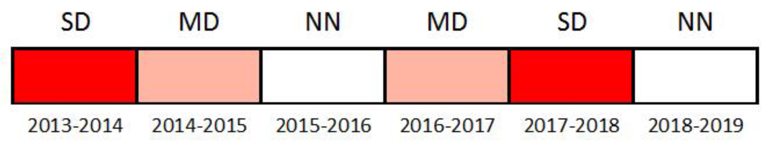
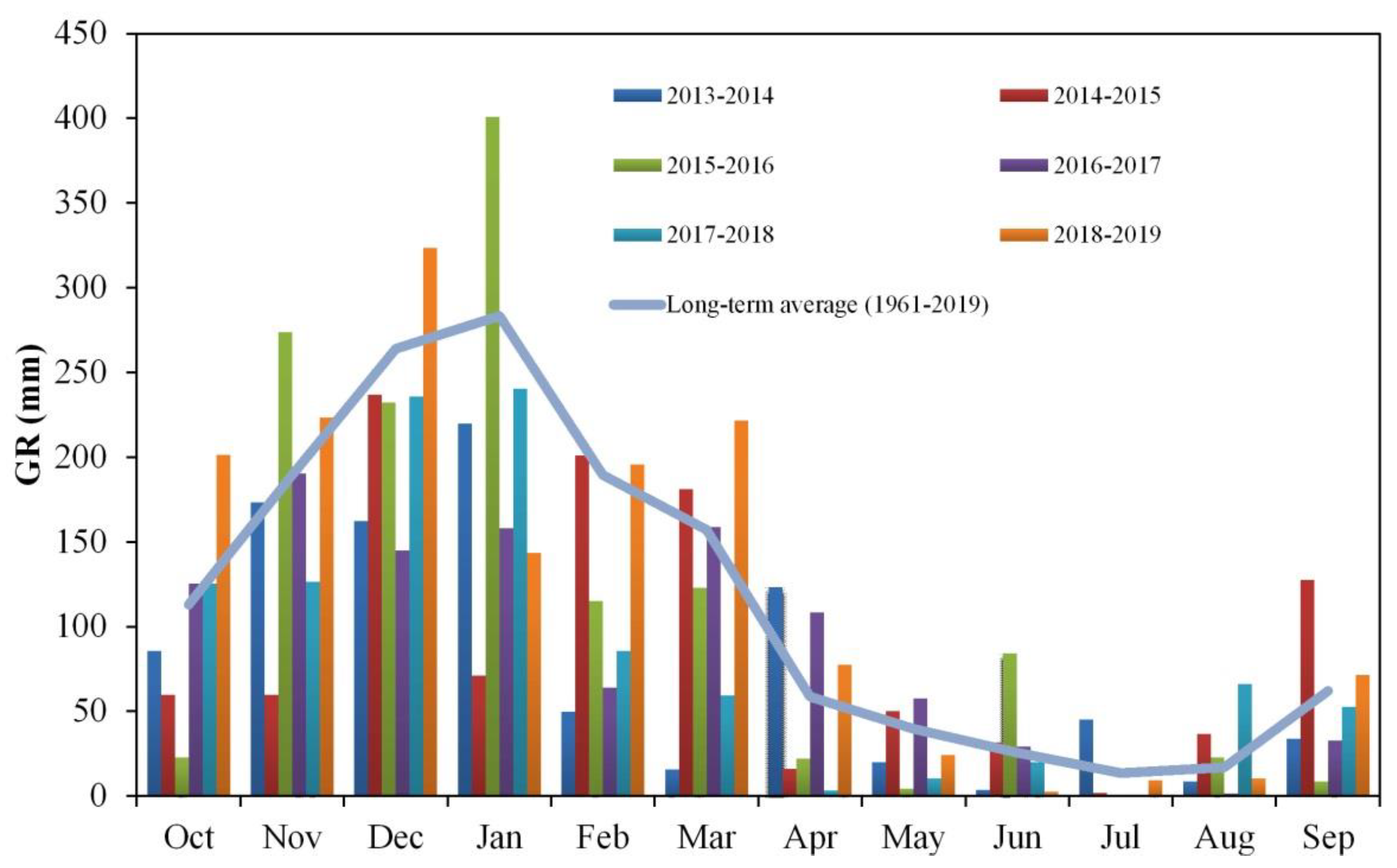
3.1. Gross Rainfall Patterns

The long-term time series used by [37] to calculate the SPI was applied to appraise the patterns of monthly gross rainfall (GR) in the study period (Figure 3). The long-term hydrological-year GR (1961–2019) was 1415 mm. The severely dry years (2013–2014 and 2017–2018) had the lowest GR amount (941 and 1025 mm, respectively), whereas the near-normal years (2015–2016 and 2018–2019) had GR close to the long-term average (1309 and 1504 mm, respectively). The moderately dry years had GR between the values 1073 mm (2014–2015) and 1070 mm (2016–2017).
Although the meteorological drought was properly classified by [37], the deficit observed in each hydrological year was due to different contributions throughout the months (Figure 3). For instance, the greatest contribution of the drought severity of 2013–2014 was the rainfall deficit in December, February, and March (summing up to −383.2 mm). On the other hand, November, February, March, and April accounted for −320.5 mm in 2017–2018. There was a significant contribution of rainfall deficit in the dry period (April to September) of 2017–2018 of −64.7 mm against +18.2 mm in 2013–2014. For the moderately dry years, November and January accounted for −342.2 mm in 2014–2015, whereas December, January, and February accounted for −370 mm in 2016–2017. However, months of GR close to or even greater than the long-term average were observed in these dry years (Figure 3). In near-normal conditions, the deficits and surplus were balanced throughout the hydrological year (Figure 2).

3.2. Energy Balance

Although gaps were observed in the meteorological time series (Figure 4), they did not preclude the energy balance analyses because the energy components were evenly distributed in the near normal, moderately dry, and severely dry periods.
Daily Rn ranged from minimal values (~0 W m−2) in the dry period (April to September) to values up to 480 W m−2 in the wet period (October to November) regardless of the drought condition (Figure 4). Minimal values of Rn were also observed in the wet period due to cloudy days. LE ranged from 0 to 400 W m−2 following the temporal behavior of Rn. This highlights the importance of energy availability for forest evapotranspiration in the study period. On the other hand, most of the H was between 0 and 50 W m−2, with some peaks up to 150 W m−2.
On average, Rn, LE, and H were 176.1 ± 87.3, 152.2 ± 80.9, and 23.8 ± 18.3 W m−2 in the near normal year, respectively; 150.9 ± 73.9, 130.8 ± 68.8, and 20.1 ± 17.6 W m−2 in the moderately dry year, respectively; and 180.1 ± 85.7, 158.5 ± 85.7, and 21.6 ± 10 W m−2 in the severely dry year, respectively. Overall, Rn, LE, and H were 169 ± 83.4, 147.1 ± 79.5, and 21.9 ± 15.9 W m−2, respectively, with LE accounting for 87% of Rn.

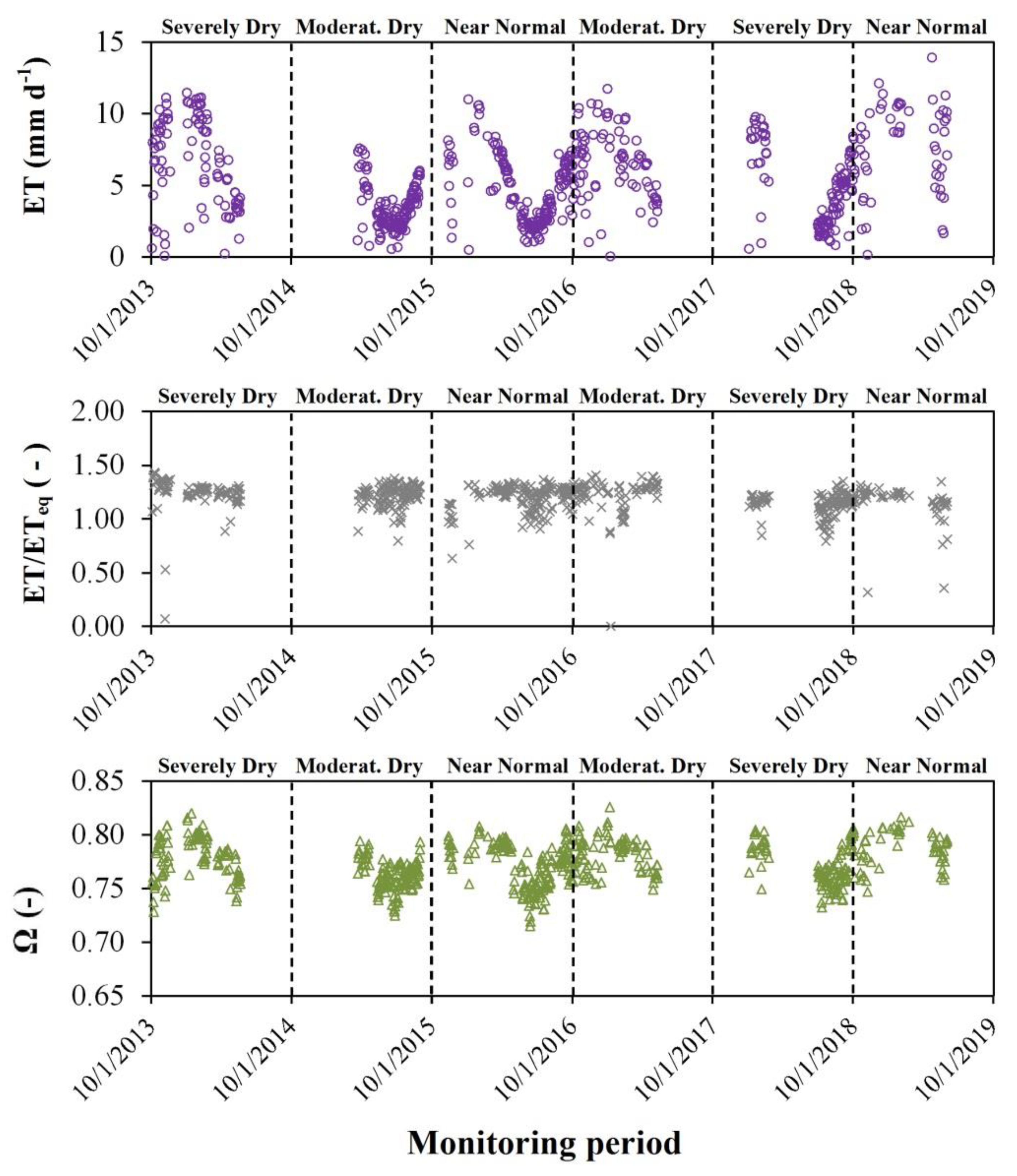
3.3. Daily Evapotranspiration (ET)

The seasonal behavior of ET followed the energy availability (Figure 4 and Figure 5). ET reached up to 14 mm d−1 in the wet period and decreased to 0.01 mm d−1 in the dry period. ET values were more grouped during the dry periods up to October, when the rainfall begins. After that, cloudy and sunny days increased the variability of ET in the wet period (Figure 5).
ET ranged from 0.12 to 14 mm d−1 in the near normal and from 0.01 to 12 mm d−1 in the moderately and severely dry conditions (Figure 6). On average, ET was 5.4 ± 2, 4.6 ± 2.1, and 5.6 ± 3.0 mm d−1 in the near normal, moderately dry, and severely dry, respectively. The ET pattern was almost the same between the periods with smaller amplitude in the moderately dry year.
Despite the difference in the rainfall patterns between the droughts [37], there was no difference in the daily VPD (Figure S2). Daily VPD ranged from 0.06 to 1.82 kPa in the near-normal conditions (Figure 7) (average of 0.73 ± 0.32 kPa). It ranged from 0.04 to 1.87 kPa in the moderately dry conditions (average of 0.61 ± 0.27 kPa); and from 0.05 to 1.94 kPa in the severely dry conditions (average of 0.77 ± 0.34 kPa). The highest values of daily VPD were observed during the wet period and in the end of the dry period.
The temporal pattern of daily Tair was the same throughout the study period (Figure 7). Tair followed the energy availability (Figure 4) and attained its maximum (28.4 °C) and minimum (11.9 °C) values in the wet and dry periods, respectively. Daily Tair averaged 22.0 ± 1.1 °C in the wet period and 19.1 ± 1.8 °C in the dry period. The same behavior was not observed for RH since air saturation and dryness occurred in both the wet and dry periods (Figure 7). This pattern is a response to the rainfall occurrence and the variability of Tair. RH ranged from 41.8% to 98.3% and averaged 71.2% ± 10% throughout the study period.
Values of ga ranged from 3.4 to 40.9 m s−1 and averaged 16.9 ± 6.3 m s−1 in the study period. There was no difference in the temporal distribution of ga between the drought conditions and the wet and dry periods. Minimum and maximum gs were ~0 and ~100 m s−1, respectively, regardless of the drought condition. These values were observed in both the dry and wet periods of every hydrological year (October to September) (Figure 7). There was a scattering of gs in the wet period due to the temporal variability of water and energy availability. On the other hand, gs values were more grouped in the end of the dry season as a consequence of few rainfall events. This indicated some seasonality of gs in the SDAF. On average, gs was 24.41 ± 20.45 m s−1.
SWS ranged from 178 to 319 mm, from 179 to 314 mm, and from 178 to 340 mm in the near normal, moderately dry, and severely dry, respectively (Figure 6). On average, SWS was 242 ± 41, 229 ± 35, and 256 ± 38 mm in the near normal, moderately dry, and severely dry, respectively. Although wetter soil conditions were observed in the severely dry years (Figure 6), the minimum values were almost the same between the periods.

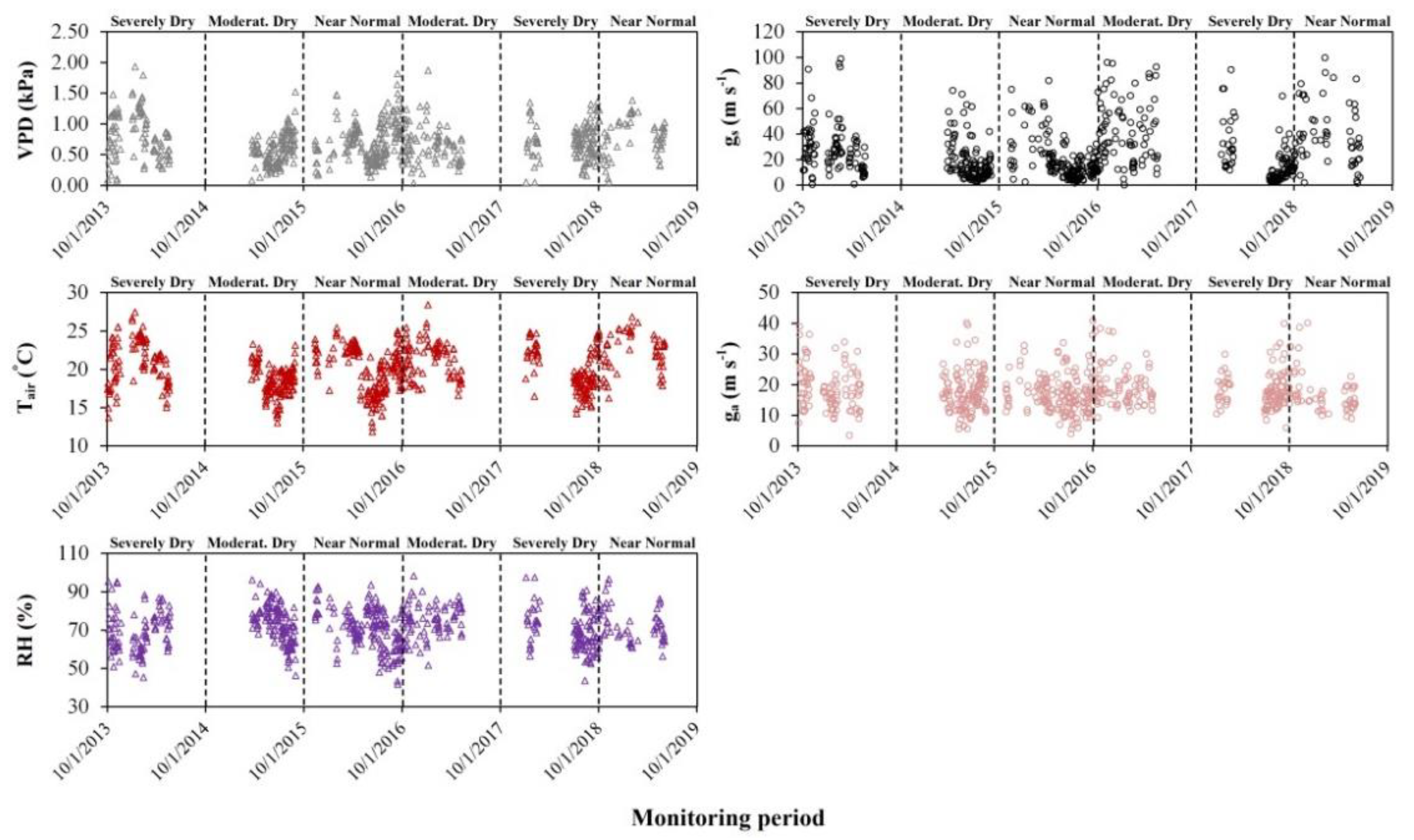
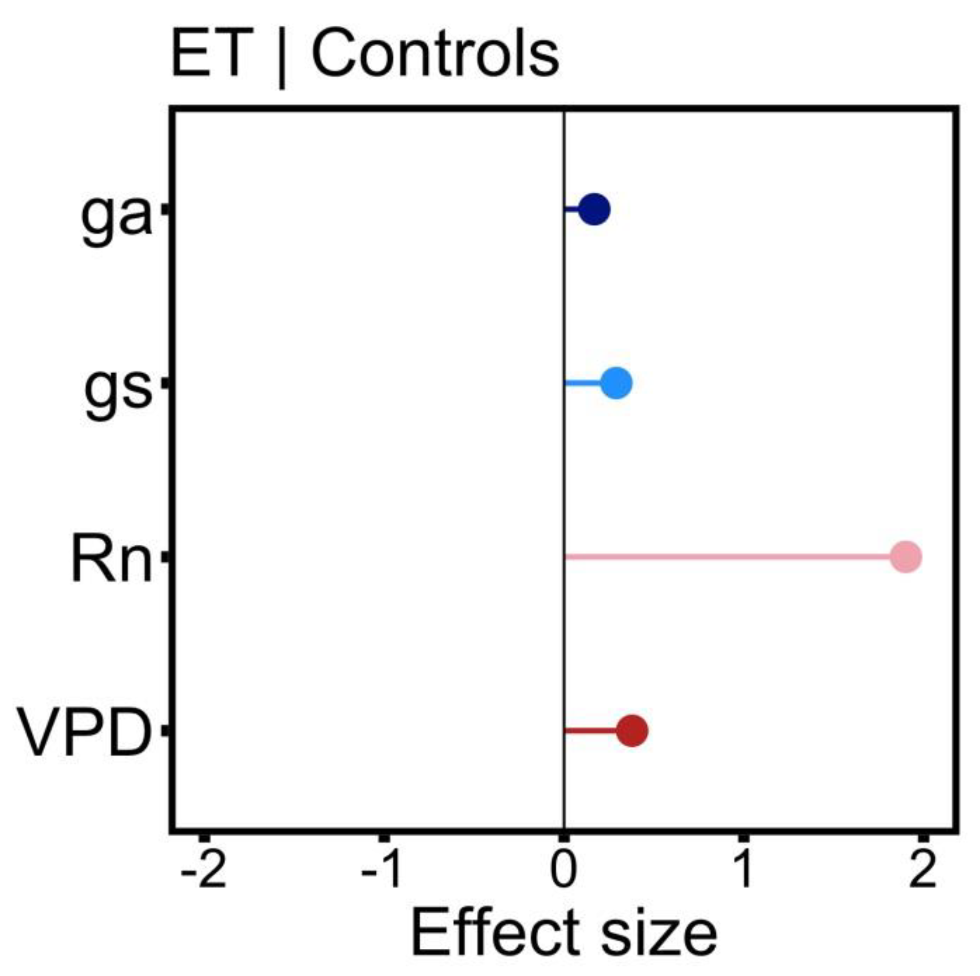
3.4. Environmental and Biophysical Controls of ET

The descriptive analyses of the monthly daily average data pointed to ga and gs as the variables with the highest and the lowest coefficient of variation in our dataset, respectively (Table 1). Moreover, a higher Pearson coefficient of correlation was observed between ET and Rn, and the lowest correlation was observed between ET and SWS (Figure 8).
The global model pointed to gs, ga, Rn, and VPD as significant explanatory variables of ET (Table 2). There was no difference in ET between the weather conditions (near normal, moderately dry, and severely dry). There was also no significant effect of SWS on ET variability.
In accordance with the global model, multimodel inference selected only one model (AIC < 2) containing gs, ga, Rn, and VPD as significant explanatory variables (Figure 9) (see the rank of models and the coefficients of the final model in Tables S1 and S2). All explanatory variables had positive effects on ET, notably Rn, which had a relatively higher influence on ET.

3.5. Priestley–Taylor and Decoupling Coefficients

The Priestley–Taylor coefficient (ET/ETeq) was basically constant throughout the study period (Figure 5), with an average of 1.20 ± 0.14. ET/ETeq > 1 highlighted the importance of energy availability and air temperature for the daily ET regardless of the weather condition. The soil moisture became a limiting factor only in a few cases when ET/ETeq < 1. In such cases, the energy radiation was basically converted to sensible heat (H) (Figure 4).
The decoupling coefficient (Ω) presented some seasonality with greater values in the wet period (Figure 5). However, the average Ω of 0.77 ± 0.02 indicated a small temporal variability. In this sense, the canopy was decoupled from the atmosphere (2013–2019) because it ranged between 0.72 and 0.82 regardless of the weather condition.

4. Discussion

4.1. Energy Balance and Daily Evapotranspiration

The temporal dynamics of LE followed Rn indicating that most of the energy availability is converted to evapotranspiration (Figure 4). This pattern is mainly observed in biomes in which soil water is not a limiting factor [50,51]. The contribution of H increases when the system changes from energy limited to water limited [5]. This was observed in the Brazilian savanna during the dry season, when the variability of LE was less correlated to Rn as soil water storage became a limiting factor [4]. The importance of H increased in a semi-evergreen tropical forest in Vietnam during a hot-dry year [50]. The greater importance of H was observed in a few days in the SDAF throughout the study period (Figure 4) and is likely related to rainless, dry, and hot days.
The daily evapotranspiration of the SDAF was in accordance with the values observed by [52] in an Atlantic Forest in the Mantiqueira range in southeastern Brazil. ET ranged from 1.53 mm d−1 (dry season) to 5.1 mm d−1 (wet season) in the Mantiqueira range, with an average of 3.26 mm d−1. The authors of [50] observed values of ET ranging from 3.64 ± 1.02 mm d−1 in the dry season to 4.65 ± 1.02 mm d−1 in the wet season in a semi-evergreen tropical forest in Vietnam. Moreover, the authors of [53] observed ET values ranging from 0.3 to 6.7 mm d−1 in the Amazon River basin. The lowest values are associated with cold weather and sparse vegetation in the Andes Cordillera, whereas the greatest ET occurred in the lowland regions characterized by abundant rainfall and tropical moist forest [53]. On the other hand, ET was lower than 2.1 mm d−1 in a semi-arid alpine step in the Tibetan Plateau [17]. Moreover, ET ranged from 0.8 o 1.3 mm d−1 in the semi-arid Caatinga in Brazil [5]. These results highlight the importance of water and energy availability for daily evapotranspiration since tropical and wet climates present greater ET.

4.2. Environmental and Biophysical Controls

ET is controlled either by the environment or by physiology and is defined by inter- and intra-annual weather variability [4], energy availability [30,54], soil moisture [4,5], soil temperature [21], vapor pressure deficit [18], stomatal dynamics [17], root depth [14], vegetation adaptation [17,19,38,50], and canopy aerodynamics [41]. Energy availability (Rn) was the main driver of ET in the seasonally dry Atlantic Forest (SDAF) (Figure 8). Rn was also the main driver of ET in arid ecosystems in China [30] and Brazil [54]; tropical evergreen forest [54], savanna [4], and wetland [51] in Brazil; and tropical rainforest in French Guiana [21], when SWS was not a limiting factor. SWS and weather condition (NN, MD, and SD) were not explanatory variables of ET in the SDAF (Figure 8). This highlights that Rn was the limiting factor of ET regardless of the drought severity.
This pattern was confirmed by the values of ET/ETeq, which indicated that ET was controlled by Rn (ET/ETeq > 1) and not by soil moisture (ET/ETeq < 1) (Figure 4). The importance of VPD and ga (Figure 9) also highlights the SWS availability, i.e., the greater the atmospheric demand (VPD) or canopy aerodynamics (ga), the greater ET. Values of Ω close to one highlighted the importance of Rn and gs to drive ET variability. gs was neither controlled by SWS nor VPD (Figure 8) since the canopy was decoupled from the atmosphere (Ω ~ 1), i.e., ET was not limited by high atmosphere demand because the soil (latosol) was able to provide water even during dry years (Figure 6). The importance of gs (Figure 9) was due to the stomatal response to the temporal variability of rainfall and energy availability (cloudy/sunny days and dry/wet periods).
The canopy coupled with the atmosphere in the dry season in the arid Caatinga in Brazil [5] highlights the control of stomatal closure (indicated by gs) in ET due to high VPD and low SWS. This was also observed in the Brazilian savanna [4], in the semi-arid alpine ecosystem in the Tibetan Plateau [17], and in a semi-evergreen tropical forest in Vietnam [50]. The stomatal closure is the first mechanism activated by vegetation to avoid water loss to the atmosphere [55]. This is followed by leaf loss and tree mortality [56] in a delayed response to persistent droughts [57]. Other mechanisms have been developed by some species to overcome droughts such as root water uptake in deep layers [14], small leaves [58], and deciduousness [59]. Such adaptations are more observed in vegetation that has naturally dry periods because increased tree mortality and a greater recovery time were observed after the 2010 drought in the humid Amazon Forest compared to a semi-arid biome in Brazil [54], i.e., humid forests suffer more with droughts because water is normally abundant. However, other ecosystems worldwide, which are somehow adapted to seasonally dry periods, had difficulties in maintaining ET in drought conditions [11,50]. These difficulties were not observed in the SDAF because of the latosol’s role in this ecosystem.
The latosol of the SDAF is a weathered soil with granular structure and micro-porosity, which confers to it a high storage capacity and infiltrability [34,38]. These capacities are boosted in the upper layers by organic matter, which was crucial for infiltration and water redistribution in the SDAF [34]. Local topography is another important factor driving soil moisture in the SDAF [34,60]. The gentle slope together with the high infiltration capacity decreased the runoff generation, which was not observed in fields (even under intense events) nor in simulations of the water balance [38]. These characteristics were crucial for maintaining ET values because SWS was stable throughout the study years (2013–2019) (Figure 6). In contrast, the Rhodic Cambisol was unable to support ET in a semi-evergreen tropical forest in Vietnam, where up to 50% of the trees lose their leaves to overcome dry periods [50]. Cambisol is shallow and linked to step topography [52,61], and therefore, it is unable to provide water as the studied latosol does.
Besides soil characteristics, the temporal distribution of rainfall and the adaptations of trees can be highlighted as other factors regularizing ET between the weather conditions. The SPI accounts for meteorological drought, which is not promptly transferred to the soil. ET and soil water redistribution are relatively slow processes [54], and it takes time for the SWS to respond to the meteorological drought. Moreover, the rainfall of some months was close to the long-term average in the moderately and severely dry years (Figure 3), which provided water inputs to the SDAF, recharging the soil. The near-normal years also contributed to maintaining soil moisture in droughts, as they represent eventual recharges of the system. This resulted in the same SWS between NN, MD, and SD years (Figure 6). Regarding the forest adaptations, more than 50% of the trees in our forest lose their leaves during the dry season [62], which naturally reduces ET on a seasonal basis and potentially make the system more resilient to drought. Moreover, the SDAF’s most abundant tree species, Xylopia brasiliensis Spreng. and Copaifera langsdorffii Desf., hold dry-affiliated traits, such as small leaves and deciduousness [24], also favoring drought-coping. Summing up, these adaptations of some tree species, the holding water capacity of the latosol, the presence of months with enough rainfall to recharge the soil, and near-normal years among droughts seem to be responsible for keeping ET only limited to energy availability (Figure 9).

4.3. Shortcomings and Implications

This study was performed considering the temporal availability of the data. Therefore, different time steps were taking depending on the data used. For instance, the coefficients (ET/ETeq and Ω) and the energy balance could be assessed in a daily step. However, the GLM was applied on the monthly averaged daily values of ET, gs, ga, and VPD because of the availability of SWS. Soil moisture was available on a monthly step because it was manually monitored. This precluded the analyses of the temporal dynamics of soil moisture and ET. However, soil moisture has been a driver of ET only when it becomes a limitation for root water uptake [4,17]. This was not the case in the SDAF since soil moisture became a limitation for ET (ET/ETeq < 1) only in a few moments throughout the study period (Figure 5). This reinforces the results of the GLM since daily ET follows the temporal behavior of Rn (Figure 4 and Figure 5). It may be interesting to decrease the temporal monitoring of soil moisture as droughts become more frequent, intense, and lasting. SWS can start being a limiting factor of ET in these conditions. Moreover, the drought was classified considering the rainfall deficit on a hydrological-year scale. The temporal distribution of rainfall within the hydrological year is another important driver of ET as one can observe different behaviors of ET and its attributes in the same drought categories (Figure 5 and Figure 7). In this sense, future studies should take into consideration the temporal distribution of GR since it is likely the cause of the different behavior of ET and its attributes in the same drought categories (NN, MD, and SD). For instance, the differences in ET (Figure 5) in the SD years (2013–2014 and 2017–2018) are likely due to the temporal distribution of GR (Figure 3), which caused different dynamics of soil moisture. However, it does not preclude the results of this study because we aimed to assess the overall condition of ET in different drought severities.
Despite the shortcomings, the importance of the water holding capacity of the latosol, monthly rainfalls to recharge the soil, and the adapted mechanism of some trees (such as small leaves and deciduousness) for regulating ET during droughts could be assessed with the available dataset. This was possible due to the time series used (six hydrological years) of daily information and a robust methodology (GLM and coefficients) to extract the most information from the dataset.
In this way, our study sheds light on the ecosystem’s characteristics that may represent sources of resilience when facing the droughts predicted in climate change scenarios. We could observe that energy availability is the great limiting factor for ET in the SDAF regardless of the drought severity. This means that the SDAF can cope with some stressful weather conditions expected in climate change scenarios. This is likely due to the soil (latosol) capacity to store water and the physiological adaptation of some trees.

5. Conclusions

ET is driven by different environmental and physiological characteristics, which can become limiting factors depending on the weather condition. Droughts can change the dynamics of ET by limiting water availability. On the other hand, energy availability (Rn) can limit ET when SWS is enough. Both the holding water capacity and the gentle topography of the dystrophic red latosol were crucial to regularizing ET in the SDAF. The values of ET/ETeq > 1 and Ω ~ 1 highlighted Rn as the limiting factor of ET regardless of the drought severity. These results were confirmed by the observed values of SWS and the results of the GLM, which did not differ between the weather conditions.
Moreover, some tree species can cope with different drought severities due to adapted mechanisms (such as deciduousness, leaf size, stomatal control, and deep water uptake). These mechanisms were developed to deal with the naturally dry periods faced by these forests. However, this ability to maintain ET in droughts was not observed in other seasonally dry forests where the soil was shallow, poorly structured, and step (e.g., Cambisol). Therefore, although physiological mechanisms are crucial for regulating water loss in dry conditions, the soil’s characteristics (such as holding water capacity and infiltrability) are fundamental to maintaining the ET even during severe droughts.
This study sheds light on the importance of the soil’s characteristics in a seasonally dry Atlantic Forest to deal with dry weather. Therefore, the decisions about the areas of the Atlantic Forest biome to be preserved (and regenerated) should take the soil into consideration, because it may define the success of the conservation area under climate change scenarios.
The main conclusions of this study can be summarized in four characteristics that drive ET dynamics:
  • Soil: the holding water and the infiltration capacities of the dystrophic red latosol were crucial to sustaining ET even in severe drought conditions.
  • Weather: Rn was the limiting factor of ET in the near-normal, moderately dry, and severely dry hydrological years.
  • Physiological mechanisms: deciduousness and small leaves were crucial for regulating water loss in dry conditions (favoring drought-coping).
  • Rainfall distribution: the inter- and intra-annual variability of gross rainfall favored soil recharge and ET.

Supplementary Materials

The following supporting information can be downloaded at https://www.mdpi.com/article/10.3390/atmos13060871/s1: Figure S1: Histogram of ET and Shapiro–Wilk normality test attesting normality. Figure S2: Box plots of daily Rn, ga, gs, and VPD in a seasonally dry Atlantic Forest under different drought periods (NN = near normal; MD = moderately dry; SD = severely dry). Table S1: GLM models of ET and the likely explanatory variables Rn, ga, gs, SWS, VPD, and period. Table S2: Explanatory variables of ET in the final GLM model.

Author Contributions

Conceptualization, D.G.-M., A.R., M.T., V.M. and C.d.M.; methodology, A.R., M.T. and S.Y.; software, A.R. and M.T.; validation, A.R., M.T. and V.M.; formal analysis, D.G.-M., A.R. and M.T.; investigation, D.G.-M., A.R. and V.M.; resources, C.d.M.; data curation, D.G.-M., A.R. and V.M.; writing—original draft preparation, D.G.-M., A.R., M.T., V.M. and C.d.M.; visualization, D.G.-M., A.R., M.T., V.M., S.Y., A.D. and C.d.M.; supervision, S.Y., A.D. and C.d.M.; project administration, C.d.M.; funding acquisition, C.d.M. All authors have read and agreed to the published version of the manuscript.

Funding

This work was supported by the Improvement of Higher Educational Personnel—CAPES [grant number: 88882.306661/2018-01] and FAPEMIG [grant number PPMX-545/18].

Institutional Review Board Statement

Not applicable.

Informed Consent Statement

Not applicable.

Data Availability Statement

The data presented in this study are available on request from the corresponding author.

Conflicts of Interest

The authors declare no conflict of interest.

Abbreviations

TermAbbreviation
EvapotranspirationET
Generalized linear modelsGLMs
Net radiationRn
Bulk surface conductancegs
Aerodynamic conductancega
Atlantic ForestAF
Soil water storageSWS
Vapor pressure deficitVPD
Seasonally dry Atlantic Forest remnantSDAF
Standard Precipitation IndexSPI
Near normalNN
Moderately dryMD
Severely drySD
Latent heat fluxλE
Sensible heat fluxH
Soil heat fluxG
Dry air densityρ
Specific heat capacity of airCp
Temperature above the forest canopyTair
Temperature within the forestTf
von Kárman’s constantk
Wind velocityu
Height of wind velocity monitoringz
Roughness length for momentum transferZ0M
Roughness length for heat transferZ0H
Zero-plane displacement heightd
Slope of saturation vapor pressure curveΔ
Psychrometric constantγ
Soil moistureθ
Soil layer thicknessh
Akaike information criterionAIC
Priestley–Taylor coefficientET/ETeq
Equilibrium evapotranspirationETeq
Decoupling coefficientΩ
Gross rainfallGR

References

  1. Allen, R.G.; Jensen, M.E.; Wright, J.L.; Burman, R.D. Operational Estimates of Reference Evapotranspiration. Agron. J. 1989, 81, 650–662. [Google Scholar] [CrossRef]
  2. Zhang, L.; Traore, S.; Cui, Y.; Luo, Y.; Zhu, G.; Liu, B.; Fipps, G.; Karthikeyan, R.; Singh, V. Assessment of Spatiotemporal Variability of Reference Evapotranspiration and Controlling Climate Factors over Decades in China Using Geospatial Techniques. Agric. Water Manag. 2019, 213, 499–511. [Google Scholar] [CrossRef]
  3. Valipour, M.; Bateni, S.M.; Sefidkouhi, M.A.G.; Raeini-Sarjaz, M.; Singh, V.P. Complexity of Forces Driving Trend of Reference Evapotranspiration and Signals of Climate Change. Atmosphere 2020, 11, 1081. [Google Scholar] [CrossRef]
  4. Christoffersen, B.O.; Restrepo-Coupe, N.; Arain, M.A.; Baker, I.T.; Cestaro, B.P.; Ciais, P.; Fisher, J.B.; Galbraith, D.; Guan, X.; Gulden, L.; et al. Mechanisms of Water Supply and Vegetation Demand Govern the Seasonality and Magnitude of Evapotranspiration in Amazonia and Cerrado. Agric. For. Meteorol. 2014, 191, 33–50. [Google Scholar] [CrossRef]
  5. Marques, T.V.; Mendes, K.; Mutti, P.; Medeiros, S.; Silva, L.; Perez-Marin, A.M.; Campos, S.; Lúcio, P.S.; Lima, K.; dos Reis, J.; et al. Environmental and Biophysical Controls of Evapotranspiration from Seasonally Dry Tropical Forests (Caatinga) in the Brazilian Semiarid. Agric. For. Meteorol. 2020, 287, 107957. [Google Scholar] [CrossRef]
  6. Rodrigues, A.F.; de Mello, C.R.; Nehren, U.; Pedro de Coimbra Ribeiro, J.; Alves Mantovani, V.; Marcio de Mello, J. Modeling Canopy Interception under Drought Conditions: The Relevance of Evaporation and Extra Sources of Energy. J. Environ. Manag. 2021, 292, 112710. [Google Scholar] [CrossRef] [PubMed]
  7. Finlayson-Pitts, J.B.; Pitts, J., Jr. Chemistry of the Upper and Lower Atmosphere: Theory, Experiments, and Applications; Academic Press: San Diego, CA, USA, 2000. [Google Scholar]
  8. Díaz-Torres, J.J.; Hernández-Mena, L.; Murillo-Tovar, M.A.; León-Becerril, E.; López-López, A.; Suárez-Plascencia, C.; Aviña-Rodriguez, E.; Barradas-Gimate, A.; Ojeda-Castillo, V. Assessment of the Modulation Effect of Rainfall on Solar Radiation Availability at the Earth’s Surface. Meteorol. Appl. 2017, 24, 180–190. [Google Scholar] [CrossRef] [Green Version]
  9. Monteith, J. Evaporation and Environment. Symposia of the Society for Experimental Biology. Symp. Soc. Exp. Biol. 1965, 19, 205–234. [Google Scholar]
  10. Kramer, P.J.; Boyer, J.S. Water Relations of Plants and Soils; Academic Press: San Diego, CA, USA, 1995. [Google Scholar]
  11. Yue, P.; Zhang, Q.; Ren, X.; Yang, Z.; Li, H.; Yang, Y. Environmental and Biophysical Effects of Evapotranspiration in Semiarid Grassland and Maize Cropland Ecosystems over the Summer Monsoon Transition Zone of China. Agric. Water Manag. 2022, 264, 107462. [Google Scholar] [CrossRef]
  12. Hu, Y.; Xiang, W.; Schäfer, K.V.R.; Lei, P.; Deng, X.; Forrester, D.I.; Fang, X.; Zeng, Y.; Ouyang, S.; Chen, L.; et al. Photosynthetic and Hydraulic Traits Influence Forest Resistance and Resilience to Drought Stress across Different Biomes. Sci. Total Environ. 2022, 828, 154517. [Google Scholar] [CrossRef]
  13. Williams, L.J.; Bunyavejchewin, S.; Baker, P.J. Deciduousness in a Seasonal Tropical Forest in Western Thailand: Interannual and Intraspecific Variation in Timing, Duration and Environmental Cues. Oecologia 2008, 155, 571–582. [Google Scholar] [CrossRef] [PubMed] [Green Version]
  14. Broedel, E.; Tomasella, J.; Cândido, L.A.; von Randow, C. Deep Soil Water Dynamics in an Undisturbed Primary Forest in Central Amazonia: Differences between Normal Years and the 2005 Drought. Hydrol. Process. 2017, 31, 1749–1759. [Google Scholar] [CrossRef]
  15. Markewitz, D.; Devine, S.; Davidson, E.A.; Brando, P.; Nepstad, D.C. Soil Moisture Depletion under Simulated Drought in the Amazon: Impacts on Deep Root Uptake. New Phytol. 2010, 187, 592–607. [Google Scholar] [CrossRef] [PubMed]
  16. De Terra, M.C.N.S.; Dos Santos, R.M.; Do Prado Júnior, J.A.; de Mello, J.M.; Scolforo, J.R.S.; Fontes, M.A.L.; Schiavini, I.; dos Reis, A.A.; Bueno, I.T.; Magnago, L.F.S.; et al. Water Availability Drives Gradients of Tree Diversity, Structure and Functional Traits in the Atlantic–Cerrado–Caatinga Transition, Brazil. J. Plant Ecol. 2018, 11, 803–814. [Google Scholar] [CrossRef] [Green Version]
  17. Ma, N.; Zhang, Y.; Guo, Y.; Gao, H.; Zhang, H.; Wang, Y. Environmental and Biophysical Controls on the Evapotranspiration over the Highest Alpine Steppe. J. Hydrol. 2015, 529, 980–992. [Google Scholar] [CrossRef]
  18. Rubert, G.C.D.; de Souza, V.A.; Zimmer, T.; Veeck, G.P.; Mergen, A.; Bremm, T.; Ruhoff, A.; de Gonçalves, L.G.G.; Roberti, D.R. Patterns and Controls of the Latent and Sensible Heat Fluxes in the Brazilian Pampa Biome. Atmosphere 2022, 13, 23. [Google Scholar] [CrossRef]
  19. Igarashi, Y.; Katul, G.G.; Kumagai, T.; Yoshifuji, N.; Sato, T.; Tanaka, N.; Tanaka, K.; Fujinami, H.; Suzuki, M.; Tantasirin, C. Separating Physical and Biological Controls on Long-Term Evapotranspiration Fluctuations in a Tropical Deciduous Forest Subjected to Monsoonal Rainfall. J. Geophys. Res. Biogeosci. 2015, 120, 1262–1278. [Google Scholar] [CrossRef] [Green Version]
  20. Loescher, H.W.; Gholz, H.L.; Jacobs, J.M.; Oberbauer, S.F. Energy Dynamics and Modeled Evapotranspiration from a Wet Tropical Forest in Costa Rica. J. Hydrol. 2005, 315, 274–294. [Google Scholar] [CrossRef]
  21. Aguilos, M.; Stahl, C.; Burban, B.; Hérault, B.; Courtois, E.; Coste, S.; Wagner, F.; Ziegler, C.; Takagi, K.; Bonal, D. Interannual and Seasonal Variations in Ecosystem Transpiration and Water Use Efficiency in a Tropical Rainforest. Forests 2019, 10, 14. [Google Scholar] [CrossRef] [Green Version]
  22. Morellato, P.C.; Haddad, C.F.B. Introduction: The Brazilian Atlantic Forest. Biotropica 2000, 32, 786–792. [Google Scholar] [CrossRef]
  23. Pires, A.P.F.; Shimamoto, C.Y.; Padgurschi, M.C.G.; Scarano, F.R.; Marques, M.C.M. Atlantic Forest: Ecosystem Services Linking People and Biodiversity. In The Atlantic Forest; Springer International Publishing: Cham, Switzerland, 2021; pp. 347–367. [Google Scholar]
  24. Mantovani, V.A.; de Terra, M.C.N.S.; de Mello, C.R.; Rodrigues, A.F.; de Oliveira, V.A.; Pinto, L.O.R. Spatial and Temporal Patterns in Carbon and Nitrogen Inputs by Net Precipitation in Atlantic Forest, Brazil. For. Sci. 2022, 68, 113–124. [Google Scholar] [CrossRef]
  25. Lira, P.K.; Tambosi, L.R.; Ewers, R.M.; Metzger, J.P. Land-Use and Land-Cover Change in Atlantic Forest Landscapes. For. Ecol. Manag. 2012, 278, 80–89. [Google Scholar] [CrossRef]
  26. de Lima, R.A.F.; Oliveira, A.A.; Pitta, G.R.; de Gasper, A.L.; Vibrans, A.C.; Chave, J.; ter Steege, H.; Prado, P.I. The Erosion of Biodiversity and Biomass in the Atlantic Forest Biodiversity Hotspot. Nat. Commun. 2020, 11, 6347. [Google Scholar] [CrossRef] [PubMed]
  27. Rezende, C.L.; Scarano, F.R.; Assad, E.D.; Joly, C.A.; Metzger, J.P.; Strassburg, B.B.N.; Tabarelli, M.; Fonseca, G.A.; Mittermeier, R.A. From Hotspot to Hopespot: An Opportunity for the Brazilian Atlantic Forest. Perspect. Ecol. Conserv. 2018, 16, 208–214. [Google Scholar] [CrossRef]
  28. Coelho, C.A.S.; de Oliveira, C.P.; Ambrizzi, T.; Reboita, M.S.; Carpenedo, C.B.; Campos, J.L.P.S.; Tomaziello, A.C.N.; Pampuch, L.A.; de Custódio, M.S.; Dutra, L.M.M.; et al. The 2014 Southeast Brazil Austral Summer Drought: Regional Scale Mechanisms and Teleconnections. Clim. Dyn. 2016, 46, 3737–3752. [Google Scholar] [CrossRef]
  29. Macedo, T.M.; da Costa, W.S.; das Brandes, A.F.N.; Valladares, F.; Barros, C.F. Diversity of Growth Responses to Recent Droughts Reveals the Capacity of Atlantic Forest Trees to Cope Well with Current Climatic Variability. For. Ecol. Manag. 2021, 480, 118656. [Google Scholar] [CrossRef]
  30. Liu, Q.; Wang, T.; Han, Q.; Sun, S.; Liu, C.; Chen, X. Diagnosing Environmental Controls on Actual Evapotranspiration and Evaporative Fraction in a Water-Limited Region from Northwest China. J. Hydrol. 2019, 578, 124045. [Google Scholar] [CrossRef]
  31. Souza, C.R.; Maia, V.A.; de Aguiar-Campos, N.; Santos, A.B.M.; Rodrigues, A.F.; Farrapo, C.L.; Gianasi, F.M.; de Paula, G.G.P.; Fagundes, N.C.A.; Silva, W.B.; et al. Long-Term Ecological Trends of Small Secondary Forests of the Atlantic Forest Hotspot: A 30-Year Study Case. For. Ecol. Manag. 2021, 489, 119043. [Google Scholar] [CrossRef]
  32. IBGE. Manual Técnico da Vegetação Brasileira, 2nd ed.; IBGE: Rio de Janeiro, Brazil, 2012; ISBN 9788524042720.
  33. Vitória, A.P.; Alves, L.F.; Santiago, L.S. Atlantic Forest and Leaf Traits: An Overview. Trees-Struct. Funct. 2019, 33, 1535–1547. [Google Scholar] [CrossRef]
  34. Junqueira Junior, J.A.; Mello, C.R.; Owens, P.R.; Mello, J.M.; Curi, N.; Alves, G.J. Time-Stability of Soil Water Content (SWC) in an Atlantic Forest-Latosol Site. Geoderma 2017, 288, 64–78. [Google Scholar] [CrossRef]
  35. Junqueira Junior, J.A.; de Mello, C.R.; de Mello, J.M.; Scolforo, H.F.; Beskow, S.; McCarter, J. Rainfall Partitioning Measurement and Rainfall Interception Modelling in a Tropical Semi-Deciduous Atlantic Forest Remnant. Agric. For. Meteorol. 2019, 275, 170–183. [Google Scholar] [CrossRef]
  36. INMET Instituto Nacional de Meteorologia. Normais Climatológicas-1991–2020. Available online: https://portal.inmet.gov.br/normais (accessed on 1 April 2022).
  37. Rodrigues, A.F.; Terra, M.C.N.S.; Mantovani, V.A.; Cordeiro, N.G.; Ribeiro, J.P.C.; Guo, L.; Nehren, U.; Mello, J.M.; Mello, C.R. Throughfall Spatial Variability in a Neotropical Forest: Have We Correctly Accounted for Time Stability? J. Hydrol. 2022, 608, 127632. [Google Scholar] [CrossRef]
  38. Rodrigues, A.F.; de Mello, C.R.; Terra, M.C.N.S.; Beskow, S. Water Balance of an Atlantic Forest Remnant under a Prolonged Drought Period. Cienc. Agrotecnol. 2021, 45, 1–13. [Google Scholar] [CrossRef]
  39. WMO. World Meteorological Organization: Standardized Precipitation Index User Guide. Available online: http://www.wamis.org/agm/pubs/SPI/WMO_1090_EN.pdf (accessed on 1 April 2022).
  40. Van Dijk, A.I.J.M.; Gash, J.H.; Van Gorsel, E.; Blanken, P.D.; Cescatti, A.; Emmel, C.; Gielen, B.; Harman, I.N.; Kiely, G.; Merbold, L.; et al. Rainfall Interception and the Coupled Surface Water and Energy Balance. Agric. For. Meteorol. 2015, 214–215, 402–415. [Google Scholar] [CrossRef] [Green Version]
  41. Tan, Z.; Zhao, J.; Wang, G.; Chen, M.; Yang, L.; He, C.; Restrepo-Coupe, N.; Peng, S.; Liu, X.; Rocha, H. Surface conductance for evapotranspiration of tropical forests: Calculations, variations, and controls. Agric. For. Meteorol. 2019, 275, 317–328. [Google Scholar] [CrossRef]
  42. Brutsaert, W. Evaporation into the Atmosphere: Theory, History and Applications; Springer: Dordrecht, The Netherlands, 1982; 302p. [Google Scholar]
  43. Stewart, J.B. Modelling Surface Conductance of Pine Forest. Agric. For. Meteorol. 1988, 43, 19–35. [Google Scholar] [CrossRef]
  44. Burnham, K.P.; Anderson, D.R. Model Selection and Inference: A Practical Information-Theoretic Approach, 2nd ed.; Springer: New York, NY, USA, 2002. [Google Scholar]
  45. Vierling, L.A.; Vierling, K.T.; Adam, P.; Hudak, A.T. Using satellite and airborne LiDAR to model woodpecker habitat occupancy at the landscape scale. PLoS ONE 2013, 8, e80988. [Google Scholar] [CrossRef] [Green Version]
  46. Barton, K. MuMIn: Multi-model inference. In R Package Version 1.46.0; R Foundation for Statistical Computing: Vienna, Austria, 2022; Available online: https://CRAN.R-project.org/package=MuMIn (accessed on 1 April 2022).
  47. R Core Team. R: A Language and Environment for Statistical Computing; R Foundation for Statistical Computing: Vienna, Austria, 2021; Available online: https://www.R-project.org/ (accessed on 1 April 2022).
  48. Wilson, K.B.; Baldocchi, D.D. Seasonal and Interannual Variability of Energy Fluxes over a Broadleaved Temperate Deciduous Forest in North America. Agric. For. Meteorol. 2000, 100, 1–18. [Google Scholar] [CrossRef]
  49. Jarvis, P.G.; Mcnaughton, K.G. Stomatal Control of Transpiration: Scaling up from Leaf to Region. Adv. Ecol. Res. 1986, 15, 1–49. [Google Scholar] [CrossRef]
  50. Kuricheva, O.A.; Avilov, V.K.; Dinh, D.B.; Sandlersky, R.B.; Kuznetsov, A.N.; Kurbatova, J.A. Seasonality of Energy and Water Fluxes in a Tropical Moist Forest in Vietnam. Agric. For. Meteorol. 2021, 299, 108268. [Google Scholar] [CrossRef]
  51. Silva, J.B.; Valle Junior, L.C.G.; Faria, T.O.; Marques, J.B.; Dalmagro, H.J.; Nogueira, J.S.; Vourlitis, G.L.; Rodrigues, T.R. Temporal Variability in Evapotranspiration and Energy Partitioning over a Seasonally Flooded Scrub Forest of the Brazilian Pantanal. Agric. For. Meteorol. 2021, 308–309, 108559. [Google Scholar] [CrossRef]
  52. Mello, C.R.; Ávila, L.F.; Lin, H.; Terra, M.C.N.S.; Chappell, N.A. Water Balance in a Neotropical Forest Catchment of Southeastern Brazil. Catena 2019, 173, 9–21. [Google Scholar] [CrossRef] [Green Version]
  53. Da Paca, V.H.M.; Espinoza-Dávalos, G.E.; Hessels, T.M.; Moreira, D.M.; Comair, G.F.; Bastiaanssen, W.G.M. The Spatial Variability of Actual Evapotranspiration across the Amazon River Basin Based on Remote Sensing Products Validated with Flux Towers. Ecol. Process. 2019, 8, 6. [Google Scholar] [CrossRef] [Green Version]
  54. Jiang, Y.; Yang, M.; Liu, W.; Mohammadi, K.; Wang, G. Eco-Hydrological Responses to Recent Droughts in Tropical South America. Environ. Res. Lett. 2022, 17, 024037. [Google Scholar] [CrossRef]
  55. Agurla, S.; Gahir, S.; Munemasa, S.; Murata, Y.; Raghavendra, A.S. Mechanism of Stomatal Closure in Plants Exposed to Drought and Cold Stress. In Advances in Experimental Medicine and Biology; Springer: Berlin/Heidelberg, Germany, 2018; Volume 1081, pp. 215–232. ISBN 9789811312441. [Google Scholar]
  56. Choat, B.; Brodribb, T.J.; Brodersen, C.R.; Duursma, R.A.; López, R.; Medlyn, B.E. Triggers of Tree Mortality under Drought. Nature 2018, 558, 531–539. [Google Scholar] [CrossRef] [PubMed]
  57. Feldpausch, T.R.; Phillips, O.L.; Brienen, R.J.W.; Gloor, E.; Lloyd, J.; Malhi, Y.; Alarcón, A.; Dávila, E.Á.; Andrade, A.; Aragao, L.E.O.C.; et al. Amazon Forest Response to Repeated Droughts. Glob. Biochem. Cycles 2016, 30, 964–982. [Google Scholar] [CrossRef]
  58. Matos, I.S.; Eller, C.B.; Oliveiras, I.; Mantuano, D.; Rosado, B.H.P. Three eco-physiological strategies of response to drought maintain the form and function of a tropical montane grassland. J. Ecol. 2020, 109, 327–341. [Google Scholar] [CrossRef]
  59. Vico, G.; Dralle, D.; Feng, X.; Thompson, S.; Manzoni, S. How Competitive Is Drought Deciduousness in Tropical Forests? A Combined Eco-Hydrological and Eco-Evolutionary Approach. Environ. Res. Lett. 2017, 12, 065006. [Google Scholar] [CrossRef] [Green Version]
  60. Oliveira, V.A.; Rodrigues, A.F.; Morais, M.A.V.; de Terra, M.C.N.S.; Guo, L.; de Mello, C.R. Spatiotemporal Modelling of Soil Moisture in an Atlantic Forest through Machine Learning Algorithms. Eur. J. Soil Sci. 2021, 72, 1969–1987. [Google Scholar] [CrossRef]
  61. Khokhlova, O.S.; Myakshina, T.N.; Kuznetsov, A.N.; Gubin, S.V. Morphogenetic Features of Soils in the Cat Tien National Park, Southern Vietnam. Eurasian Soil Sci. 2017, 50, 158–175. [Google Scholar] [CrossRef]
  62. Terra, M.C.N.S.; Mello, C.R.; Mello, J.M.; Oliveira, V.A.; Nunes, M.H.; Silva, V.O.; Rodrigues, A.F.; Alves, G.J. Stemflow in a Neotropical Forest Remnant: Vegetative Determinants, Spatial Distribution and Correlation with Soil Moisture. Trees-Struct. Funct. 2018, 32, 323–335. [Google Scholar] [CrossRef]
Figure 1. The geographical location of Atlantic Forest original cover in Brazil (a), the location of the seasonally dry Atlantic Forest (b) with the positions of soil moisture measuring points (c), and the two meteorological stations, one below the canopy (d) and other above the canopy (e).
Atmosphere 13 00871 g001
Figure 2. Graphical representation of the droughts’ classification of the hydrological years according to SPI [37] in the SDAF. SD = severely dry; MD = moderately dry; NN = near normal.
Atmosphere 13 00871 g002
Figure 3. Monthly rainfall of each hydrological year (2013 to 2019) and the long-term average in the seasonally dry Atlantic Forest (SDAF).
Atmosphere 13 00871 g003
Figure 4. Seasonal variation of the net radiation (Rn) (upper figure), latent heat flux (LE) (middle figure), and sensible heat flux (H) (lower figure) in six hydrological years (2013 to 2019) in different weather conditions (severely dry, moderately dry, and near normal).
Atmosphere 13 00871 g004
Figure 5. Seasonal variation of the daily evapotranspiration (ET) (upper figure), the Priestley–Taylor coefficient (ET/ETeq) (middle figure) and the decoupling coefficient (Ω) (lower figure) in six hydrological years (2013 to 2019) in different weather conditions (severely dry, moderately dry, and near normal).
Atmosphere 13 00871 g005
Figure 6. Box plots of daily evapotranspiration (ET) (left figure) and monthly soil water storage (SWS) (right figure) in a seasonally dry Atlantic Forest (SDAF) under different drought conditions (NN = near normal; MD = moderately dry; SD = severely dry).
Atmosphere 13 00871 g006
Figure 7. Seasonal variation of the vapor pressure deficit (VPD) (upper left), air temperature (Tair) (middle left), relative humidity (RH) (lower left), bulk surface conductance (gs) (upper right), and aerodynamic conductance (ga) (middle right) in six hydrological years (2013 to 2019) in different weather conditions (severely dry, moderately dry, and near normal).
Atmosphere 13 00871 g007
Figure 8. Pearson correlation coefficients among monthly averaged of daily evapotranspiration (ET), bulk surface conductance (gs), aerodynamic conductance (ga), net radiation (Rn), vapor pressure deficit (VPD), soil water storage (SWS) for the 2013–2019 period in the seasonally dry Atlantic Forest (SDAF). Insignificant coefficients (p > 0.05) are marked with an “X”. Dataset used in the statistical modeling.
Atmosphere 13 00871 g008
Figure 9. Drivers of evapotranspiration (ET) in the seasonally dry Atlantic Forest (SDAF) indicated by the generalized linear models (GLM). The size of the bars represents the scaling effect of each variable.
Atmosphere 13 00871 g009
Table 1. Descriptive analyses of the monthly daily average of evapotranspiration (ET), bulk surface conductance (gs), aerodynamic conductance (ga), net radiation (Rn), vapor pressure deficit (VPD), and soil water storage (SWS) for the 2013–2019 period in a seasonally dry Atlantic tropical forest. Dataset used in the statistical modeling.
MeanStandard DeviationCoefficient of Variation
ET6.062.4340.05
gs29.2314.3349.03
ga18.023.0316.81
Rn196.0575.3738.44
VPD0.740.2533.99
SWS251.4341.4416.48
Table 2. Generalized linear model (global model) of monthly daily average evapotranspiration (ET) against the explanatory variables period, bulk surface conductance (gs), aerodynamic conductance (ga), net radiation (Rn), vapor pressure deficit (VPD), and soil water storage (SWS) for the 2013–2019 period in the seasonally dry Atlantic Forest (SDAF). Estimate: Variable coefficient, (…); significance: 0 = ‘***’; 0.01 = ‘*’.
EstimateStd. Errort ValuePr(>|t|)Significance
Intercept5.5536190.16992232.6834.45 × 10−16 ***
MD−0.0071540.189232−0.0380.970311
SD0.102240.1852520.5520.588643
gs0.3122870.0732844.2610.000597***
ga0.1644580.0594972.7640.013826*
Rn1.8717960.09738419.2211.76 × 10−12***
VPD0.3841680.0771474.980.000136***
SWS0.0113480.0723570.1570.877338
Publisher’s Note: MDPI stays neutral with regard to jurisdictional claims in published maps and institutional affiliations.

