Article

Combining Sun-Photometer, PM Monitor and SMPS to Inverse the Missing Columnar AVSD and Analyze Its Characteristics in Central China

1
School of Remote Sensing and Information Engineering, Wuhan University, Wuhan 430079, China
2
State Key Laboratory of Information Engineering in Surveying, Mapping and Remote Sensing, Wuhan University, Wuhan 430079, China
3
Electronic Information School, Wuhan University, Wuhan 430079, China
*
Authors to whom correspondence should be addressed.
Atmosphere 2022, 13(6), 915; https://doi.org/10.3390/atmos13060915
Submission received: 4 May 2022 / Revised: 1 June 2022 / Accepted: 2 June 2022 / Published: 5 June 2022
(This article belongs to the Topic Recent Progress in Aerosol Remote Sensing and Products)

Abstract

:
Columnar aerosol volume size distribution (AVSD) is an important atmospheric parameter that shows aerosol microphysical properties and can be used to analyze the impact of aerosols on the radiation budget balance, as well as regional climate effects. Usually, columnar AVSD can be obtained by using a sun photometer, but its observation conditions are relatively strict, and the columnar AVSD will be missing in cloudy or hazy weather due to cloud cover and other factors. This study introduces a novel algorithm for inversion of missing columnar AVSD under haze periods by using a machine learning approach and other ground-based observations. The principle is as follows. We are based on joint observational experiments. Since the scanning mobility particle sizer (SMPS) and particulate matter (PM) monitor sample the surface data, they can be stitched together to obtain the surface AVSD according to their observation range. Additionally, the sun-photometer scans the whole sky, so it can obtain columnar AVSD and aerosol optical depth (AOD). Then we use the back propagation neural network (BPNN) model to establish the relationship between the surface AVSD and the columnar AVSD and add AOD as a constraint. Next, the model is trained with the observation data of the same period. After the model training is completed, the surface AVSD and AOD can be used to invert the missing columnar AVSD during the haze period. In experiments on the 2015 dataset, the results show that the correlation coefficient and root mean square error between our model inversion results and the original sun photometer observations were 0.967 and 0.008 in winter, 0.968 and 0.010 in spring, 0.969 and 0.013 in summer, 0.972 and 0.007 in autumn, respectively. It shows a generally good performance that can be applied to the four seasons. Furthermore, the method was applied to fill the missing columnar AVSD of Wuhan, a city in central China, under adverse weather conditions. The final results were shown to be consistent with the climatic characteristics of Wuhan. Therefore, it can indeed solve the problem that sun photometer observations are heavily dependent on weather conditions, contributing to a more comprehensive study of the effects of aerosols on climate and radiation balance.

1. Introduction

Aerosol refers to a gaseous dispersion system consisting of solid or liquid particles suspended in a gaseous medium. Aerosol particles, ranging in diameter from 1 nm to 100 µm, can absorb and scatter solar radiation to affect regional and global climate [1,2]. In addition, they will make the atmosphere turbid, reduce visibility, be inhaled and deposited in the respiratory tract, alveoli, etc., to cause disease when the particle size is less than 10 µm [3,4]. There are two ways in which atmospheric aerosols are produced, the first is natural phenomena, including sand and dust, ocean waves, and volcanic eruptions. For example, Tonga’s submarine volcano erupted on 15 January 2022. According to a report by the Fiji Environment Department on 17 January, satellite data showed that the sky of Tonga and surrounding countries was covered with a large amount of volcanic ash and gas, and the concentration of aerosols in the atmosphere increased dramatically [5]. The resulting aerosol particles, which are also ejected into the stratosphere and circle the Earth several times, have a long lifespan, and studies have shown that they have a surface cooling effect [6]. The second is anthropogenic activities, including combustion, industrial emissions, and gas-to-particle conversion [7,8]. The aerosol particles produced in this way have a great impact on human health and are also the main cause of air pollution [9]. Wuhan, a metropolis in central China, is facing many environmental pressures from population growth and industrial development, so man-made pollution raises the concentration of aerosols and contributes to the haze. Although the government has made great efforts to control smog, haze incidents have occurred from time to time. At the same time, apart from the Beijing–Tianjin–Hebei region, the Yangtze River Delta region, and the Pearl River Delta region, central China is also the main region for haze events [10,11,12,13]. When haze occurs, the concentration of fine aerosol particles in the atmosphere will increase, and these fine particles will affect the formation of clouds and thus affect precipitation, and indirectly affect the Earth’s radiation balance and regional climate [14]. During this period, we can understand the formation and diffusion mechanism of haze by studying multiple atmospheric parameters, which can provide an effective reference for haze management [15].
The columnar AVSD (aerosol volume size distribution) is one of the most important aerosol microphysical parameters. It is not only a key indicator of environmental quality but also of great significance for understanding the physical and chemical properties of aerosols [16,17]. Therefore, obtaining columnar AVSD during haze is very important for haze management. Typically, columnar AVSD can be obtained by retrieving data from remote sensors such as LiDAR, sun photometer, or sky radiometer. Nowadays, more and more universities and research institutes are using CIMEL sun photometers and joining AERONET (Aerosol Robotics Network) as the core detection network of radiometers and gaining wide impact. As a result, columnar AVSD inversions using sun photometers have been widely used and Dubovik’s method has become the standard algorithm [18]. However, inversion of the aerosol particle size spectrum distribution requires sky scattered light, so the observation conditions are highly influential, and it is difficult to perform an inversion on cloudy days when the sky scattered light is weak [19,20,21]. For these reasons, we cannot obtain columnar AVSD data from sun photometers during periods of high aerosol concentration such as haze. Although the country has paid attention to environmental management in recent years and achieved outstanding results, the aerosol concentration in China and Southeast Asia is still high [22,23], and we have to overcome this problem to obtain better results. In view of this, it is important to obtain the solution for inversion of columnar AVSD at high aerosol concentrations. What is more, many observation stations and observation networks have been built in China [24]. If the columnar AVSD of a single site is filled, it is believed that the practical application value of the stations and observation networks can be more effectively utilized.
In response to the above problems, this study proposes a novel algorithm for the inversion of columnar AVSD. First, based on the joint observation experiment, the columnar AVSD and AOD (aerosol optical depth) were obtained through the sun-photometer, and the surface AVSD was obtained from the joint data of SMPS (scanning mobility particle sizer) and PM (particulate matter) monitor. The second step was to obtain the surface and columnar AVSD distribution parameters through the least squares fitting. Then, the parameters are brought into the BPNN (Back Propagation Neural Network) model for training to obtain the best model. Finally, when we cannot obtain the columnar AVSD from the sun photometer in bad weather conditions, the AOD and surface AVSD can be used to inverse the missing columnar AVSD, which will fill in the gap. In this way, a more complete set of atmospheric parameters can be obtained, which plays a very important role in the study of not only haze control but also climate effects in central China.

2. Observational Instruments and Methodology

The three instruments used in this study, including a sun-photometer from CIMEL (France), a PM monitor from GRIMM (Germany), and a SMPS from TSI (USA), are located at the State Key Laboratory of Information Engineering in Surveying, Mapping and Remote Sensing (LIESMARS; 30°32′ N, 114°21′ E) in Wuhan (Figure 1). Wuhan is the capital city of Hubei province and is located in central China at the confluence of the Yangtze and Han rivers [25]. We also use atmospheric monitoring data from the Wuhan Environmental Monitoring Center, through which we obtain reliable PM2.5 (particles less than 2.5 μm in diameter) observation records. In this study, we propose a novel algorithm to invert the sky columnar AVSD during the haze period by combining three instruments for simultaneous observations.

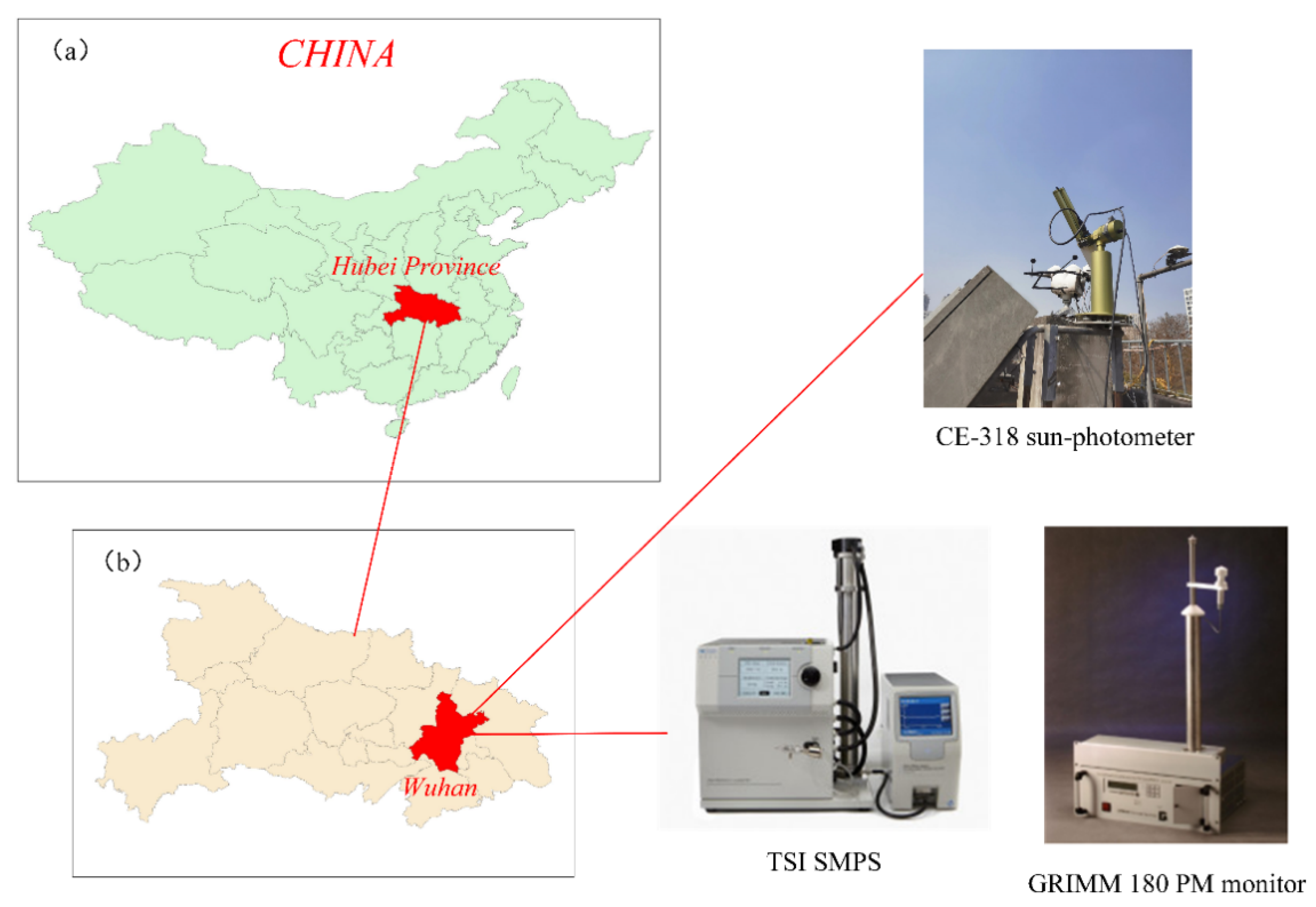
2.1. Observational Instruments

The CE-318 sun photometer is an automatic tracking and scanning solar radiometer. The instrument has nine spectral channels in the visible near-infrared band with central wavelengths of 340 nm, 380 nm, 440 nm, 500 nm, 670 nm, 870 nm, 936 nm, 1020 nm, and 1640 nm, respectively. It measures direct solar radiation by automatically tracking the sun’s position and can characterize aerosol properties from the solar almucantar. Solar radiation data measured by the CE-318 sun photometer can also derive atmospheric transmittance, extinction optical thickness, AOD, precipitation column amounts, and ozone concentration [26,27]. The instrument is calibrated following the AERONET calibration protocol method once a year to ensure the accuracy and reliability of the observed data. A detailed description of the instrument calibration is presented by Che et al. [28,29,30].
The GRIMM 180 PM monitor was used to conduct online measurements of aerosol concentrations, which can collect real-time measurements of both aerosol concentrations for 31 particle-size segments and mass concentrations of PM1, PM2.5, and PM10. The requirements of the instrument for the sampling gas are: temperature between −20–60 °C, relative humidity below 95%, and no dew. After obtaining the sampling gas the particle size distribution of the particulate material is measured continuously by light scattering. Assuming that the particulate matter is spherical, it then calculates the mass from the volume distribution so obtained [31,32].
The TSI SMPS is often used to measure size distribution of nanoparticles in the airborne particles, and it requires an operating environment of 10–40 °C and 10–90% humidity. The main component of the SMPS is an electrostatic classifier (ESC) which includes a differential mobility analyzer (DMA), and a condensation particle counter (CPC). In the ESC polydisperse particles are separated according to their electrical mobility. At each specific voltage, only particles with a specific electrical mobility are capable of passing through the DMA into a butanol-based CPC where the particles are counted. An exponential sweep of the voltage applied to the inner cylinder of the DMA was then performed to obtain the size distribution of the aerosol [33].
In summary, we can obtain columnar AVSD and AOD by using a sun photometer. The TSI SMPS measures fine aerosol particles, its measurement range is 0.01–0.66 μm, while the GRIMM 180 PM monitor can measure aerosol coarse particles, its measurement range is 0.25–32 μm, so the two instruments can be combined to obtain a wider range surface AVSD. The units for the surface AVSD and columnar AVSD are μm3/μm3 and μm3/μm2, respectively.

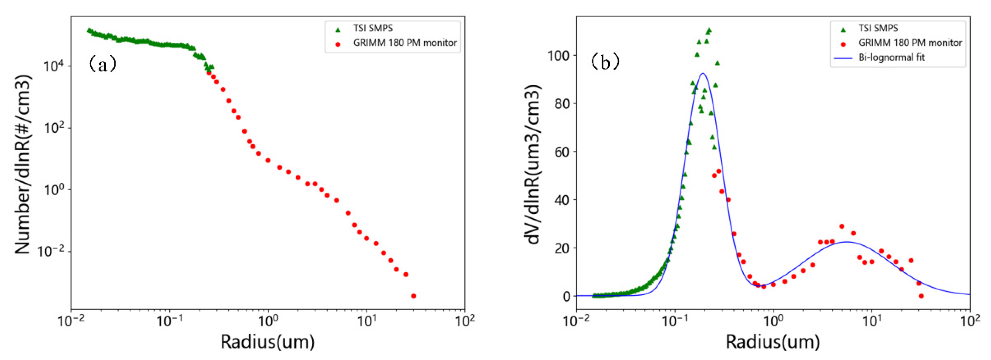
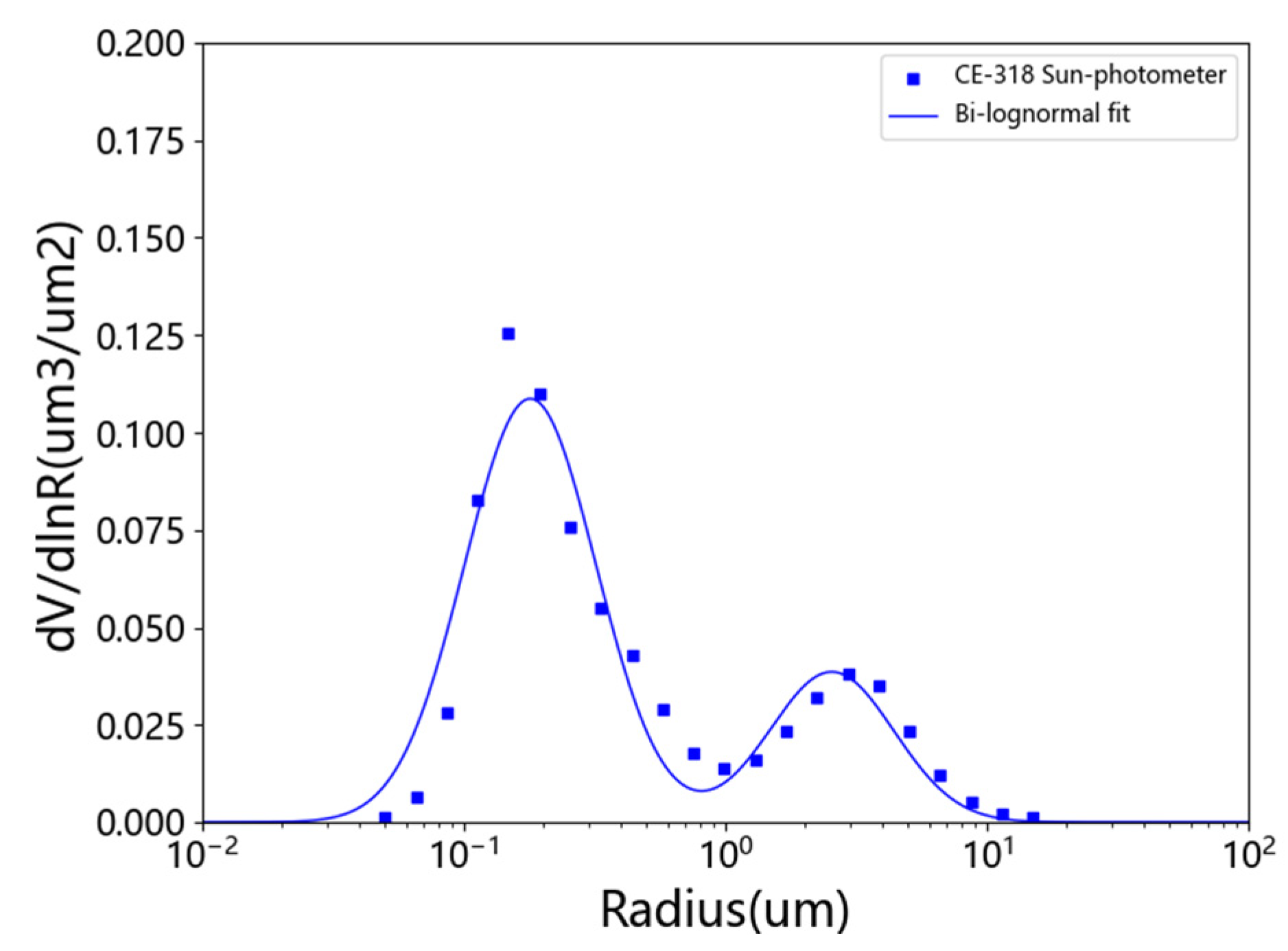
2.2. Retrieval Principle

We usually use the conventional AVSD inversion method proposed by King et al. in 1978 to obtain the aerosol size distribution. The AOD of multiple wavelengths is determined by light extinction of direct sunlight measured by the sun photometer [34], assuming that the aerosol particles are homogeneously distributed spherical particles, so the AOD can therefore be expressed using Mie theory as
τ ( λ ) = r m i n r m a x π r 2 Q e ( r , λ , m ) N ( r ) d r
where r is the radius of the aerosol particles; rmax and rmin denote the maximum radius and the minimum radius of the radius range, respectively; Qe(r,λ,m) is the extinction efficiency factor in accordance with Mie theory; λ corresponds to the wavelength of the incident illumination; m represents the complex refractive index, and N(r) is the unknown columnar aerosol number size distribution (ANSD).
N(r) is related to dV(r)/dln(r) in the following way:
N ( r )   r   ( 4 3 π r 3 ) = d V ( r ) d l n ( r )
where V(r) is the columnar AVSD density in the radius range r to r + dr with V(r) = (4π/3) r3 N(r); dV(r)/dln(r) is the aerosol volume size distribution. Thus, Function (1) can be also written as
τ ( λ ) = 3 4   r m i n r m a x Q e ( r , λ , m ) r 2 d V ( r ) d l n ( r ) d r
According to Function (3), the AVSD can be inverted when the AOD is known, but the traditional inversion method of King et al. (1978) makes a lot of assumptions and performs a lot of manual intervention, which makes the results highly uncertain.

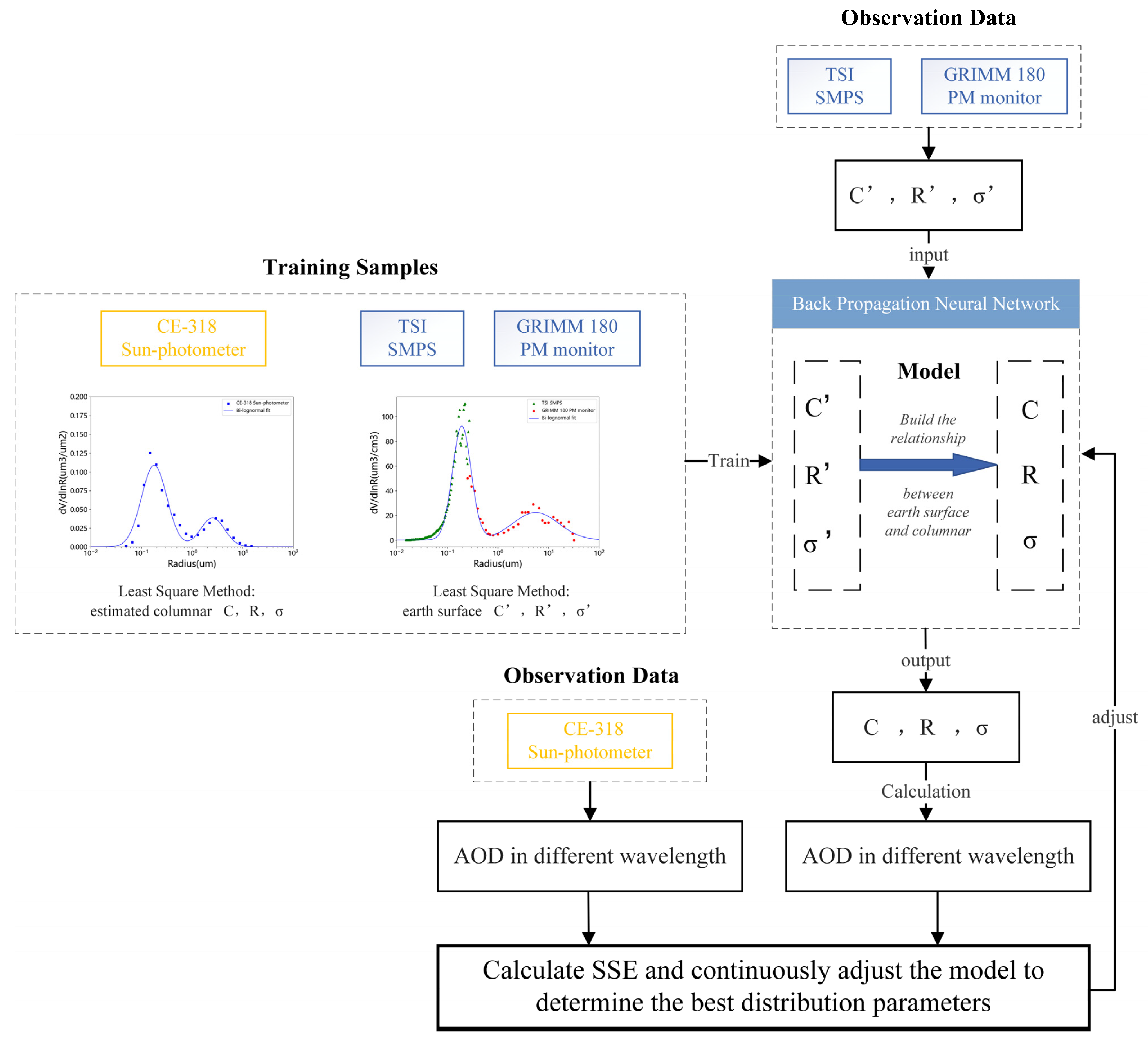
3. Novel Algorithm Combined with Machine Learning
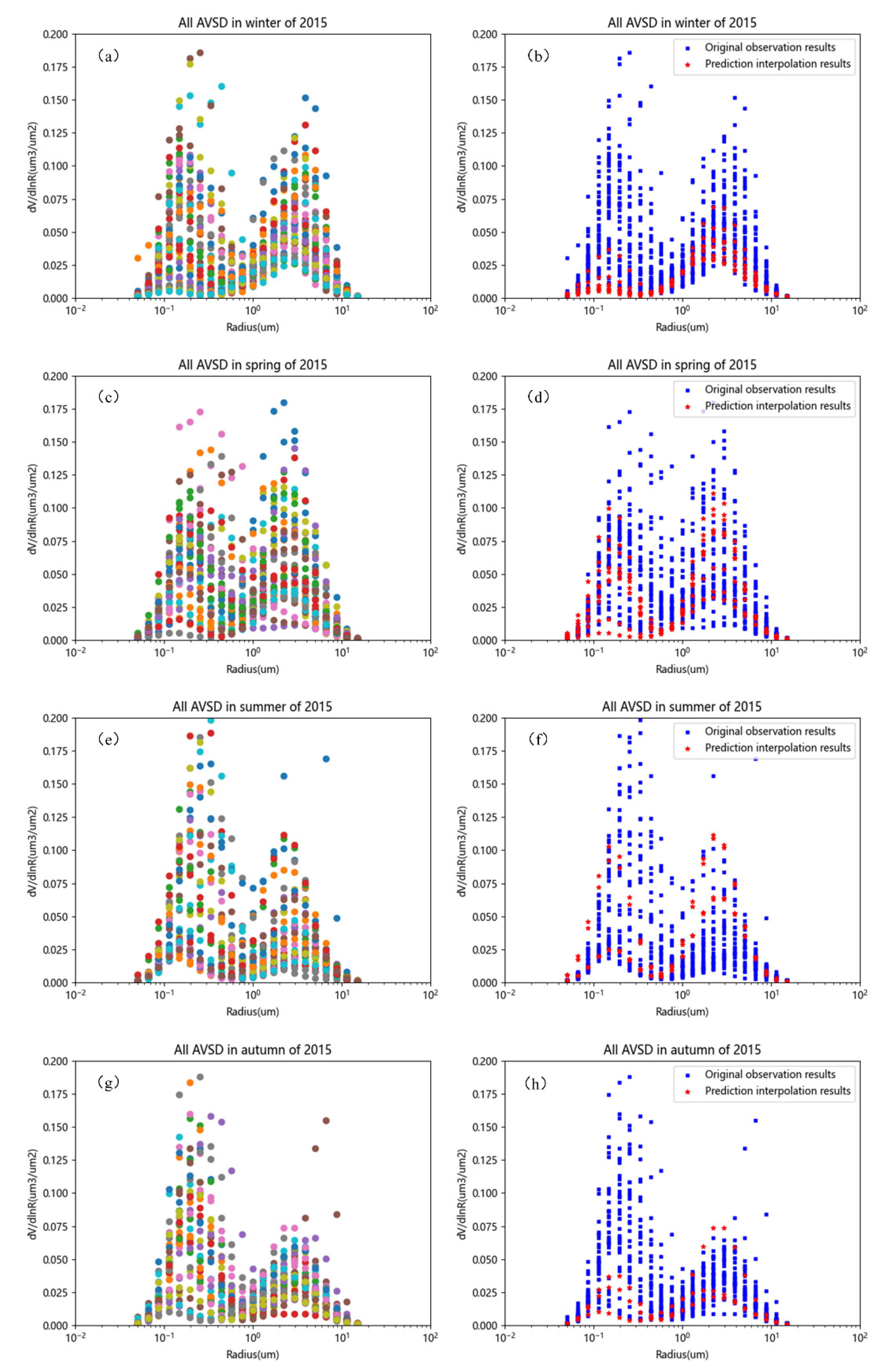
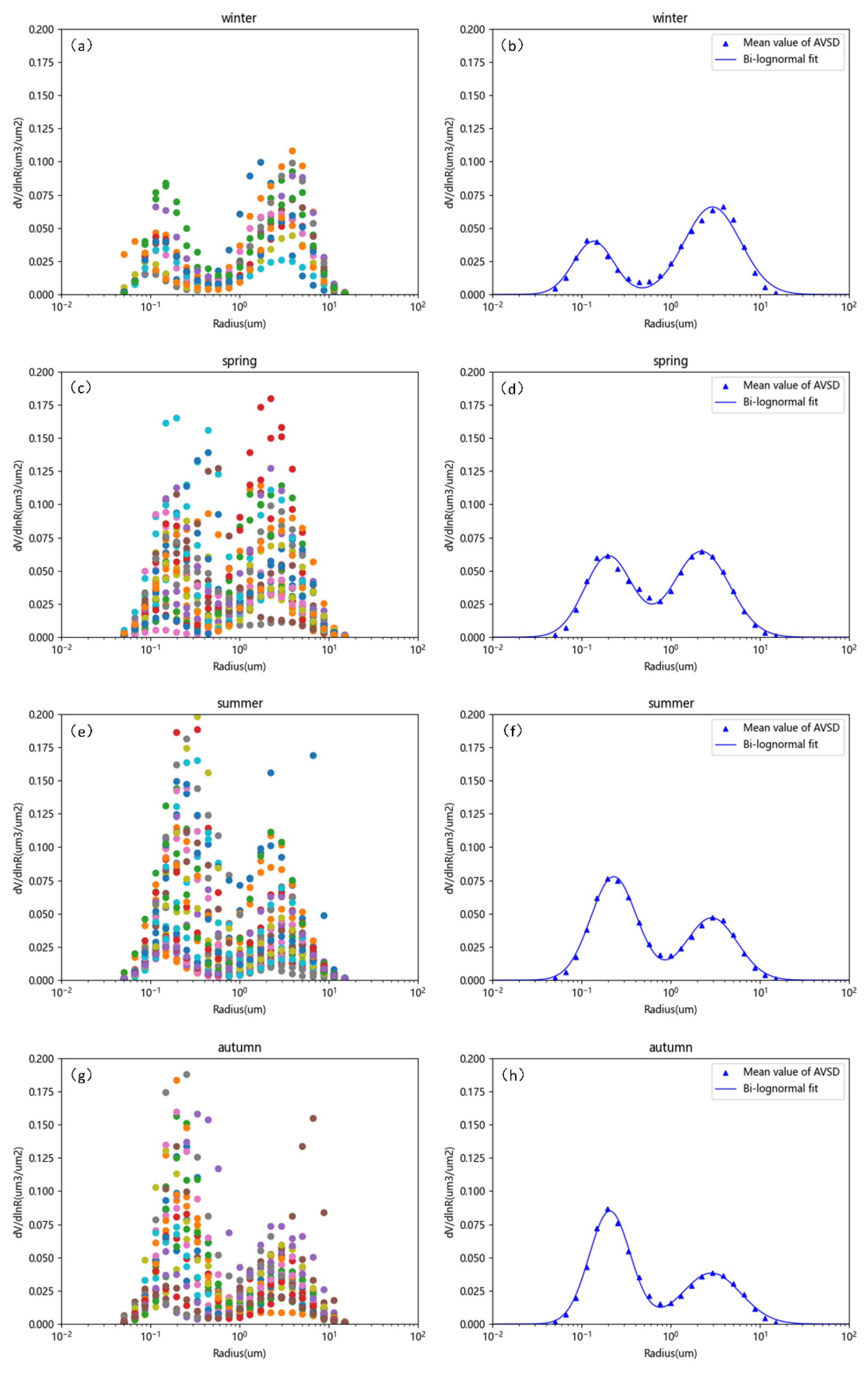
In order to fill in the observation data of monitoring instruments during the haze period in Wuhan and provide an effective reference for the management of haze, this section introduces a novel algorithm to invert the columnar AVSD of the sun-photometer missing during haze.
The particle size distribution refers to the number of particles contained within different particle radii. Many studies have shown that the aerosol distribution can usually be better represented by a bimodal normal distribution function [18,19,35], the bimodal lognormal normal distribution function can be described by Function (4):
d V ( r ) d l n ( r ) = C f 2 π σ f   exp ( ( l n r l n R f ) 2 2 σ f 2 ) + C c 2 π σ c   exp ( ( l n r l n R c ) 2 2 σ c 2 )
In Function (4) dV(r)/dln(r) indicates the volume concentration of particles in a certain particle size range, C is the particle volume concentration, R is the median radius, σ is the variance, and the subscripts f and c represent the fine and coarse particle, respectively. In other words, we just need to know C, R, and σ, and we can obtain the model constants of columnar AVSD.
The AOD τ(λ) simulated according to the Mie theory can be calculated by the above-mentioned Function (3). At this point, Qe is the extinction efficiency of dust particles calculated by the Mie program, and m is the complex refractive index of aerosol particles, which usually ranges from 1.33 to 1.6.
For a single band, we can calculate the simulated AOD based on Function (3) as a constraint to obtain C, R, σ in Function (4). When there are multiple bands, each band can obtain a simulated AOD, we can calculate the sum of squared errors (SSE) between the true AOD and modeled AOD, and continuously adjust C, R, and σ in Function (4) to minimize the SSE. The calculation equation is as follows:
Q SSE = 1 k i = 1 k ( τ m o d i τ o b s i ) 2
when the SSE reaches the minimum value, the corresponding Cf, Cc, Rf, Rc, σf, σc is the optimal solution, i.e., the most reasonable columnar AVSD.
In order to find the six distribution parameters with the smallest SSE in the above method and obtain the optimal columnar AVSD, we propose a novel algorithm that combines least squares fitting with BPNN prediction, the process of which is shown in Figure 2.
At first, we selected some AVSD training samples from both columnar and surface AVSD, which should basically satisfy the bimodal lognormal normal distribution. The six distribution parameters Cf, Cc, Rf, Rc, σf, and σc in AVSD are then obtained by fitting with the least squares method in machine learning. The least squares method is the most classical curve fitting technique in machine learning, which finds the curve that best fits the data by minimizing the square of the error and is based on the following principle.
Suppose there is a series of data values, D = {(x1, y2), (x2, y2), …, (xn, yn)}, it is necessary to find a function f(x) = ax + b, so that the output of f(x) is as close as possible to y. Then, the key to least squares is to obtain this function based on the principle of minimum variance between the predicted value and the true value. The variance is calculated by the following formula:
Q = i = 1 n ( a x i + b y i ) 2
The principle of least squares is to let Q be the smallest to find a, b. For our training sample, there are six parameters Cf, Cc, Rf, Rc, σf, and σc according to Function (4), which means finding the values of these 6 parameters when Q is the smallest.
Secondly, after obtaining the AVSD parameters of the training samples, they are brought into the BPNN model for training. The BPNN has a strong nonlinear mapping ability and flexible network structure, which has been relatively mature in both network theory and performance [36]. Its structure is shown in Figure 3. BPNN has an input layer, a hidden layer, and an output layer; in essence, the BP algorithm is to calculate the minimum value of the objective function by using the gradient descent method with the network error squared as the objective function.
The principle of the BP algorithm is as follows. The BPNN model does not need to determine the mathematical equations of the mapping relationship between input and output in advance, but only through its own training, learning some rules to obtain the closest result to the desired output value at a given input value [37]. The basic idea of the algorithm is the gradient descent method, which uses the gradient search technique to minimize the mean squared error between the actual and desired output values of the network. The basic BP algorithm consists of two processes: forward propagation of the signal and backward propagation of the error. In forward propagation, the input signal acts on the output node through the implied layer, and after nonlinear transformation, the output signal is generated, and if the actual output does not match the desired output, it is transferred to the back propagation process of the error. The error back propagation is to backpropagate the output error through the implied layer to the input layer one by one, apportion the error to all units in each layer and use the error signal obtained from each layer as the basis for adjusting the weight of each unit [38]. The network parameters (weights and thresholds) corresponding to the minimum error are determined by adjusting the connection strength of the input nodes to the hidden layer nodes and the connection strength of the hidden layer nodes to the output nodes, as well as the thresholds, so that the error decreases along the gradient direction, after repeated learning training.
In this study, we take the six parameters of the observed surface AVSD as input values and the six distribution parameters of the columnar AVSD as output values and add the observed AOD as a constraint. We select several days of data as samples to train the model, and once the model is trained, we can use the surface AVSD parameters to predict the columnar AVSD parameters. Finally, we can calculate the modeled AOD by Function (3) and then calculate the SSE between the observed AOD and the modeled AOD. According to the magnitude of the SSE, we can continue to adjust our model and finally obtain the optimal predicted columnar AVSD.

4. Results

Haze events in Wuhan usually occur in autumn and winter, so observations from three instruments were used in the winter of 2014–2015 in our experiments. During 2014–2015, the three instruments had been used for a short period of time and maintained regularly, and the data observed were very accurate. Combining the observations from the three instruments, we removed the periods for which no data were recorded by the CE-318 sun photometer and the corresponding periods for which the GRIMM 180 PM monitor and TSI SMPS data and their data records were incomplete, resulting in 35 days of available data (as shown in Table 1).
As shown in Figure 4: GRIMM 180 PM monitor and TSI SMPS acquire the surface data, and we can stitch them together based on the particle size range characteristics they observe. The two instruments obtain the aerosol particle number concentration, and according to the above, Function (2), we can convert them to volume concentration and finally obtain the surface AVSD, meanwhile, they have been shown to conform to the bimodal lognormal normal distribution, so the six distribution parameters of the surface AVSD can be obtained by least squares method fitting. As shown in Figure 5, the data obtained by the CE-318 sun photometer is the columnar AVSD, and in the same way, we can also obtain the six distribution parameters of the columnar AVSD.
According to the above method, we first obtain data for a period of time and then bring them into the BPNN model for training to establish the relationship between the surface AVSD and the columnar AVSD. Once the model is trained, we can input the surface AVSD into the model and obtain the columnar AVSD. Then, we can compare the results obtained by our novel algorithm with the original inversion result of the sun photometer, and as shown in Figure 6 we show the inversion results of our model for 30 days of winter. As shown in Table 2, we calculated the correlation coefficient (r) between the original inversion result of the sun photometer and the inversion results of our novel algorithm and recorded the PM2.5 for that day. Among them, for the records of PM2.5, we chose the data of East Lake Liyuan Station, because it is the nearest station to Wuhan University. The 2012 Chinese National Ambient Air Quality Standard (NAAQS) sets PM2.5 concentration limits for both the 24-h average and the annual mean value. The 24-h average concentration limited value is 35 μg/m3 for Category I places, including natural protection zones, scenic resorts, and other areas needing special protection, and 75 μg/m3 for all other places (Category II places) [39]. At the same time, this study also refers to the environmental air quality index (AQI) technical requirements (HJ 633–2012), and finally, we consider Wuhan has polluted weather when its daily average PM2.5 concentration exceeds 75 μg/m3.
As shown in Table 2, our novel algorithm forecasts over the 30 days of winter are very close to the original inversion result of the sun photometer. Their correlation coefficients ranged from a low of 0.93 to a high of 0.99, while they were essentially greater than 0.97. We also recorded the PM2.5 for these periods and from the results, it is clear that PM2.5 does not have a significant impact on our inversion results. On 4 January 2015, even though the PM2.5 for this day was 128, which is considered a severe haze event, the correlation coefficient of the inversion results reached 0.9938. It can also be seen from Figure 6 that the difference between the inversion results of our novel algorithm and the sun photometer is basically in the range of ±0.025, with only a very few cases exceeding this range. The inversion results show that our novel algorithm is able to overcome the influence of PM2.5 and give good results in most weather conditions. The reason for the discrepancy in the above prediction results is that the model may have been over-fitted when the samples were selected for training, making the model fit one weather condition more closely than another, or be too extreme on the day of the prediction. In these cases, we first controlled the training of the model to prevent over-fitting and added AOD constraints to allow the model to automatically adjust to conditions in different periods.
The above results show that the inversion accuracy of our model is high, and PM2.5 has no significant effect on the inversion results. However, it was only analyzed for each day’s results, so to evaluate the model more fully, we calculated the correlation coefficient (r) and root mean square error (RMSE) for a whole winter combination. Additionally, inversion only for the winter period is not sufficient to prove the feasibility of our model; therefore, we extended the period of the experiment from December 2014 (winter) to November 2015 (autumn), during which we chose four seasons for the inversion. During this time of year, January 2014 to February 2015 falls in the winter, March 2015 to May 2015 in the spring, June 2015 to August 2015 in the summer, and September 2015 to November 2015 in the autumn. We have conducted experiments on all four seasons of the year, so the experimental data is wider, can represent the characteristics of most periods, and the results are more convincing. In the inversion experiments for the four seasons, we select 2-3 days in each month of all available data in a year as training samples and the rest as test samples for prediction. Similarly, we calculated the correlation coefficients and root mean square errors for the combined inversion results for each season and recorded the total number of days of inversion experiments performed in each season. The final results are shown in Table 3.
From the inversion results of the above four seasons, we can see that our novel algorithm not only has good inversion results in a short time but also applies to long time series. However, the selection of samples has a great influence on the inversion results. If the prediction is made only for a short period, then we only need to train a small portion of the data in this period as training samples to obtain good results, but at the cost that the model we obtain may only be applicable for this small period of time. If we are making predictions for a year or several years, then we need to choose a very large training sample, such as choosing a few days in each month of the year to put together as a sample to train the model. Then, the model we obtain from the training will satisfy most of the cases, and with the AOD constraint, the model’s prediction results will be very accurate.
As mentioned above, the CE-318 sun photometer will have missing observations during the haze period and cannot obtain the columnar AVSD, so our new algorithm can be used to invert the missing columnar AVSD by using the surface AVSD obtained from the joint TSI SMPS and GRIMM 180 PM monitor observations and adding the constraint of AOD. Following on from the previous inversion experiments for the four seasons of 2015, we continued with the inversion for dates between December 2014 and November 2015. There are dates in this time period where columnar AVSD data are missing, but joint observations data from the TSI SMPS and GRIMM 180 PM monitors and AOD data are available. Therefore, we can use these known data to invert the columnar AVSD using our new algorithmic model. After inverting to obtain the missing columnar of AVSD, we inserted them into our original observation data. The final interpolation results are shown in Figure 7, where the temporal division of the seasons is the same as in the above experiment.
Although we obtained the missing columnar AVSD through model inversion and interpolated them to enrich all columnar AVSD data for each season, the data observed under clean atmosphere conditions were more consistent with the columnar AVSD characteristics of the day. Therefore, we excluded data obtained when the daily mean of PM2.5 was greater than 75. After that, we averaged and fitted all the columnar AVSD of each season, and the final result was considered to be representative of the characteristics of each season in Wuhan, as shown in Figure 8.
From the final results, it can be seen that the coarse particles are higher in winter and spring, and the fine particles are dominant in summer and autumn, which is related to the climatic characteristics of Wuhan. In winter, the accumulation of moist and cold air leads to higher water vapor content in the air, and the moisture absorption growth of aerosol particles increases the concentration of coarse particles. In spring, which is the peak of factory resumption and population movement after the Chinese New Year, man-made pollutant emissions can raise the concentration of fine particles in the atmosphere [40]. At the same time, medium-sized particles of about 1 μm in size will increase due to the long-distance transmission of sand and dust during this period [41]. In summer, with high temperatures and high air humidity, the concentration of coarse particles in the atmosphere decreases, and the concentration of fine particles increases due to the condensation effect [42,43]. In autumn, the air is relatively dry, which is conducive to the diffusion and deposition of pollutants, and the concentration of coarse particles will still decrease, while the source of the increase in fine particles is likely to be naturally generated, and the emission of pollutants. In general, the results we obtained are in line with the characteristics of Wuhan, so the above experiments are correct and feasible.

5. Discussion and Conclusions

The rapid development of the economy has led to large emissions of man-made pollutants, which not only deteriorate air quality and increase regional aerosol concentrations but also have an impact on climate change. Although the government has increased its efforts to control the problem and has achieved good results, we still need to use multiple atmospheric parameters to more deeply study and analyze aerosol characteristics and physicochemical properties. The number of sun photometers installed in China has been increasing in recent years, and many observation stations and observation networks have been established. However, due to the limitation of instrument observation conditions, there will be missing observation data under bad weather conditions. If we can fill in the missing sky columnar AVSD data using the method of this study, it is believed that this can play a greater role in the application of observation sites and observation networks.
This study used not only a sun photometer, but also a PM monitor and SMPS, and based on their combined observation experiments, we could obtain columnar AVSD, surface AVSD, and AOD. Then, a machine learning method is used to build a model to realize the process of inverting the columnar AVSD from the surface AVSD. The final results (Table 2 and Table 3) show that the correlation coefficients and root mean square errors of the inversion results of this method with the original inversion results were 0.967 and 0.008 in winter 2014, 0.968 and 0.010 in spring 2015, 0.969 and 0.013 in summer 2015, 0.972 and 0.007 in autumn 2015, respectively. This means that the algorithm has high inversion accuracy and robustness and can perform inversion under different weather conditions. What is more, the filling results of columnar AVSD interpolation for Wuhan in 2015 (Figure 8) are also in line with the climatic characteristics of Wuhan. Therefore, it is proved that our method is reliable and can be practically applied. It is worth mentioning that, based on the advantages of machine learning, the algorithm avoids the complex mathematical calculation process, can be applied to different regions and different time periods, and can use a small number of samples to invert to obtain accurate results.
Although the experimental results show that our method is very effective, it does not mean that our current work is sufficient. In the future, we consider the following ways to improve our research:
  • When training the BPNN model, over-fitting may occur, and the training results of the model are also closely related to the selection of training samples, so the model needs to be adjusted according to the actual situation. Therefore, adding PM2.5 or PM10 as a constraint to obtain an inversion model more suitable for weather conditions needs to be considered in the future.
  • We plan to add tethered balloon or sounding balloon data in the future to further verify the accuracy of our columnar AVSD inversion. In addition, the CE-318 sun photometer can only work during the daytime, unlike GRIMM 180 PM monitor and TSI SMPS, which also have nighttime monitoring data. But the surface AVSD is lower at night and higher during the day, so we cannot accurately predict the nighttime columnar AVSD..
  • Adding more atmospheric parameters is necessary to analyze and study the principles of haze formation and dispersion more comprehensively, while the aerosol types in Wuhan are complex and require longer observation data to improve our understanding of the impact of aerosols on the atmosphere and climate.
  • In bad weather conditions, we can obtain fewer data records which are not enough for long-time observation. In addition, the size range of columnar AVSD is fixed from 0.05 to 15 μm, but in fact, the size of surface AVSD obtained from our joint observations is highly variable and can range from 0.0151 to 32 μm. Therefore, exploiting a larger scale range to study the characteristics of columnar AVSD is an important topic for future research work.

Author Contributions

Conceptualization, A.M., S.J. and Y.M.; data curation, A.M., N.J. and W.H.; formal analysis, A.M.; investigation, A.M., X.Q. and Y.Z.; methodology, A.M., S.J. and Y.M.; project administration, A.M. and Y.M.; resources, S.J., Y.M and B.L.; validation, A.M., S.J. and Y.M.; visualization, A.M.; writing—original draft, A.M.; writing—review and editing, S.J., Y.M. and B.L. All authors have read and agreed to the published version of the manuscript.

Funding

This research was funded by the National Key R&D Program of China (Grant No. 2018YFB0504500), National Natural Science Foundation of China (Grant No. 41875038, No. 42071348, and No. 42001291), the Key R&D projects in Hubei Province (Grant No. 2021BCA220) and supported by LIESMARS Special Research Funding.

Institutional Review Board Statement

Not applicable.

Informed Consent Statement

Not applicable.

Data Availability Statement

Data available on request due to their restrictions on public sharing.

Acknowledgments

We thank the editors and reviewers for their comments that help us improve the manuscript.

Conflicts of Interest

The authors declare no conflict of interest.

References

  1. Ramanathan, V.; Crutzen, P.J.; Kiehl, J.; Rosenfeld, D. Aerosols, climate, and the hydrological cycle. Science 2001, 294, 2119–2124. [Google Scholar] [CrossRef] [Green Version]
  2. Che, H.; Xia, X.; Zhu, J.; Li, Z.; Dubovik, O.; Holben, B.; Goloub, P.; Chen, H.; Estelles, V.; Cuevas-Agulló, E. Column aerosol optical properties and aerosol radiative forcing during a serious haze-fog month over North China Plain in 2013 based on ground-based sunphotometer measurements. Atmos. Chem. Phys. 2014, 14, 2125–2138. [Google Scholar] [CrossRef] [Green Version]
  3. Charlson, R.J.; Schwartz, S.; Hales, J.; Cess, R.D.; Coakley, J., Jr.; Hansen, J.; Hofmann, D. Climate forcing by anthropogenic aerosols. Science 1992, 255, 423–430. [Google Scholar] [CrossRef] [PubMed]
  4. Baker, K.R.; Foley, K.M. A nonlinear regression model estimating single source concentrations of primary and secondarily formed PM2.5. Atmos. Environ. 2011, 45, 3758–3767. [Google Scholar] [CrossRef]
  5. Adam, D. Tonga volcano eruption created puzzling ripples in Earth’s atmosphere. Nature 2022, 601, 497. [Google Scholar] [CrossRef] [PubMed]
  6. Aubry, T.J.; Staunton-Sykes, J.; Marshall, L.R.; Haywood, J.; Abraham, N.L.; Schmidt, A. Climate change modulates the stratospheric volcanic sulfate aerosol lifecycle and radiative forcing from tropical eruptions. Nat. Commun. 2021, 12, 4708. [Google Scholar] [CrossRef]
  7. Huang, R.-J.; Zhang, Y.; Bozzetti, C.; Ho, K.-F.; Cao, J.-J.; Han, Y.; Daellenbach, K.R.; Slowik, J.G.; Platt, S.M.; Canonaco, F. High secondary aerosol contribution to particulate pollution during haze events in China. Nature 2014, 514, 218–222. [Google Scholar] [CrossRef] [Green Version]
  8. Ding, A.; Huang, X.; Nie, W.; Sun, J.; Kerminen, V.M.; Petäjä, T.; Su, H.; Cheng, Y.; Yang, X.Q.; Wang, M. Enhanced haze pollution by black carbon in megacities in China. Geophys. Res. Lett. 2016, 43, 2873–2879. [Google Scholar] [CrossRef]
  9. World Health Organization. Health Aspects of Air Pollution: Results from the WHO Project “Systematic Review of Health Aspects of Air Pollution in Europe”; WHO: Geneva, Switzerland, 2004. [Google Scholar]
  10. Chameides, W.L.; Yu, H.; Liu, S.; Bergin, M.; Zhou, X.; Mearns, L.; Wang, G.; Kiang, C.; Saylor, R.; Luo, C. Case study of the effects of atmospheric aerosols and regional haze on agriculture: An opportunity to enhance crop yields in China through emission controls? Proc. Natl. Acad. Sci. USA 1999, 96, 13626–13633. [Google Scholar] [CrossRef] [Green Version]
  11. Li, Z.; Xia, X.; Cribb, M.; Mi, W.; Holben, B.; Wang, P.; Chen, H.; Tsay, S.C.; Eck, T.; Zhao, F. Aerosol optical properties and their radiative effects in northern China. J. Geophys. Res. Atmos. 2007, 112. [Google Scholar] [CrossRef]
  12. Chen, J.; Xin, J.; An, J.; Wang, Y.; Liu, Z.; Chao, N.; Meng, Z. Observation of aerosol optical properties and particulate pollution at background station in the Pearl River Delta region. Atmos. Res. 2014, 143, 216–227. [Google Scholar] [CrossRef]
  13. Xia, X.; Li, Z.; Holben, B.; Wang, P.; Eck, T.; Chen, H.; Cribb, M.; Zhao, Y. Aerosol optical properties and radiative effects in the Yangtze Delta region of China. J. Geophys. Res. Atmos. 2007, 112. [Google Scholar] [CrossRef]
  14. Wang, H.-J.; Chen, H.-P. Understanding the recent trend of haze pollution in eastern China: Roles of climate change. Atmos. Chem. Phys. 2016, 16, 4205–4211. [Google Scholar] [CrossRef] [Green Version]
  15. Liu, X.; Li, J.; Qu, Y.; Han, T.; Hou, L.; Gu, J.; Chen, C.; Yang, Y.; Liu, X.; Yang, T. Formation and evolution mechanism of regional haze: A case study in the megacity Beijing, China. Atmos. Chem. Phys. 2013, 13, 4501–4514. [Google Scholar] [CrossRef] [Green Version]
  16. Ma, Y.; Gong, W.; Wang, L.; Zhang, M.; Chen, Z.; Li, J.; Yang, J. Inversion of the haze aerosol sky columnar AVSD in central China by combining multiple ground observation equipment. Opt. Express 2016, 24, 8170–8185. [Google Scholar] [CrossRef]
  17. Liu, B.; Ma, X.; Ma, Y.; Li, H.; Jin, S.; Fan, R.; Gong, W. The relationship between atmospheric boundary layer and temperature inversion layer and their aerosol capture capabilities. Atmos. Res. 2022, 271, 106121. [Google Scholar] [CrossRef]
  18. Dubovik, O.; King, M.D. A flexible inversion algorithm for retrieval of aerosol optical properties from Sun and sky radiance measurements. J. Geophys. Res. Atmos. 2000, 105, 20673–20696. [Google Scholar] [CrossRef] [Green Version]
  19. King, M.D.; Byrne, D.M.; Herman, B.M.; Reagan, J.A. Aerosol size distributions obtained by inversions of spectral optical depth measurements. J. Atmos. Sci. 1978, 35, 2153–2167. [Google Scholar] [CrossRef]
  20. Böckmann, C. Hybrid regularization method for the ill-posed inversion of multiwavelength lidar data in the retrieval of aerosol size distributions. Appl. Opt. 2001, 40, 1329–1342. [Google Scholar] [CrossRef]
  21. Nakajima, T.; Tonna, G.; Rao, R.; Boi, P.; Kaufman, Y.; Holben, B. Use of sky brightness measurements from ground for remote sensing of particulate polydispersions. Appl. Opt. 1996, 35, 2672–2686. [Google Scholar] [CrossRef]
  22. Chen, X.; Wang, Z.; Li, J.; Yang, W.; Chen, H.; Wang, Z.; Hao, J.; Ge, B.; Wang, D.; Huang, H. Simulation on different response characteristics of aerosol particle number concentration and mass concentration to emission changes over mainland China. Sci. Total Environ. 2018, 643, 692–703. [Google Scholar] [CrossRef] [PubMed]
  23. Liu, S.; Xing, J.; Zhao, B.; Wang, J.; Wang, S.; Zhang, X.; Ding, A. Understanding of aerosol–climate interactions in China: Aerosol impacts on solar radiation, temperature, cloud, and precipitation and its changes under future climate and emission scenarios. Curr. Pollut. Rep. 2019, 5, 36–51. [Google Scholar] [CrossRef]
  24. Goloub, P.; Li, Z.; Dubovik, O.; Blarel, L.; Podvin, T.; Jankowiak, I.; Lecoq, R.; Deroo, C.; Chatenet, B.; Morel, J. PHOTONS/AERONET Sunphotometer Network Overview: Description, Activities, Results. Available online: https://doi.org/10.1117/12.783171 (accessed on 1 June 2022).
  25. Cheng, J.; Masser, I. Urban growth pattern modeling: A case study of Wuhan city, PR China. Landsc. Urban Plan. 2003, 62, 199–217. [Google Scholar] [CrossRef]
  26. Dubovik, O.; Smirnov, A.; Holben, B.; King, M.; Kaufman, Y.; Eck, T.; Slutsker, I. Accuracy assessments of aerosol optical properties retrieved from Aerosol Robotic Network (AERONET) Sun and sky radiance measurements. J. Geophys. Res. Atmos. 2000, 105, 9791–9806. [Google Scholar] [CrossRef] [Green Version]
  27. Masoumi, A.; Khalesifard, H.; Bayat, A.; Moradhaseli, R. Retrieval of aerosol optical and physical properties from ground-based measurements for Zanjan, a city in Northwest Iran. Atmos. Res. 2013, 120, 343–355. [Google Scholar] [CrossRef]
  28. Che, H.; Zhang, X.; Chen, H.; Damiri, B.; Goloub, P.; Li, Z.; Zhang, X.; Wei, Y.; Zhou, H.; Dong, F. Instrument calibration and aerosol optical depth validation of the China Aerosol Remote Sensing Network. J. Geophys. Res. Atmos. 2009, 114. [Google Scholar] [CrossRef]
  29. Dubovik, O.; Holben, B.; Eck, T.F.; Smirnov, A.; Kaufman, Y.J.; King, M.D.; Tanré, D.; Slutsker, I. Variability of absorption and optical properties of key aerosol types observed in worldwide locations. J. Atmos. Sci. 2002, 59, 590–608. [Google Scholar] [CrossRef]
  30. Che, H.; Xia, X.; Zhu, J.; Wang, H.; Wang, Y.; Sun, J.; Zhang, X.; Shi, G. Aerosol optical properties under the condition of heavy haze over an urban site of Beijing, China. Environ. Sci. Pollut. Res. 2015, 22, 1043–1053. [Google Scholar] [CrossRef]
  31. Deng, X.; Li, F.; Li, Y.; Li, J.; Huang, H.; Liu, X. Vertical distribution characteristics of PM in the surface layer of Guangzhou. Particuology 2015, 20, 3–9. [Google Scholar] [CrossRef]
  32. Grimm, H.; Eatough, D.J. Aerosol measurement: The use of optical light scattering for the determination of particulate size distribution, and particulate mass, including the semi-volatile fraction. J. Air Waste Manag. Assoc. 2009, 59, 101–107. [Google Scholar] [CrossRef]
  33. Hogrefe, O.; Lala, G.G.; Frank, B.P.; Schwab, J.J.; Demerjian, K.L. Field evaluation of a TSI model 3034 scanning mobility particle sizer in New York City: Winter 2004 intensive campaign. Aerosol Sci. Technol. 2006, 40, 753–762. [Google Scholar] [CrossRef] [Green Version]
  34. Huang, J.; Wang, T.; Wang, W.; Li, Z.; Yan, H. Climate effects of dust aerosols over East Asian arid and semiarid regions. J. Geophys. Res. Atmos. 2014, 119, 11398–11416. [Google Scholar] [CrossRef]
  35. Remer, L.A.; Kaufman, Y.J. Dynamic aerosol model: Urban/industrial aerosol. J. Geophys. Res. Atmos. 1998, 103, 13859–13871. [Google Scholar] [CrossRef] [Green Version]
  36. Wang, Z. Optimizing BP Neural Network Prediction Model based on WOA. Int. Core J. Eng. 2021, 7, 342–348. [Google Scholar]
  37. Hecht-Nielsen, R. Theory of the backpropagation neural network. In Neural Networks for Perception; Elsevier: Amsterdam, The Netherlands, 1992; pp. 65–93. [Google Scholar]
  38. Amari, S.I. Backpropagation and stochastic gradient descent method. Neurocomputing 1993, 5, 185–196. [Google Scholar] [CrossRef]
  39. You, M. Addition of PM2.5 into the national ambient air quality standards of China and the contribution to air pollution control: The case study of Wuhan, China. Sci. World J. 2014, 2014, 768405. [Google Scholar] [CrossRef] [PubMed] [Green Version]
  40. Gong, W.; Zhang, S.; Ma, Y. Aerosol optical properties and determination of aerosol size distribution in Wuhan, China. Atmosphere 2014, 5, 81–91. [Google Scholar] [CrossRef] [Green Version]
  41. Ma, Y.; Zhang, M.; Jin, S.; Gong, W.; Chen, N.; Chen, Z.; Jin, Y.; Shi, Y. Long-Term Investigation of Aerosol Optical and Radiative Characteristics in a Typical Megacity of Central China during Winter Haze Periods. J. Geophys. Res. Atmos. 2019, 124, 12093–12106. [Google Scholar] [CrossRef]
  42. Jin, S.; Ma, Y.; Zhang, M.; Gong, W.; Lei, L.; Ma, X. Comparation of aerosol optical properties and associated radiative effects of air pollution events between summer and winter: A case study in January and July 2014 over Wuhan, Central China. Atmos. Environ. 2019, 218, 117004. [Google Scholar] [CrossRef]
  43. Liu, H.; Shao, J.; Jiang, W.; Liu, X. Numerical Modeling of Droplet Aerosol Coagulation, Condensation/Evaporation and Deposition Processes. Atmosphere 2022, 13, 326. [Google Scholar] [CrossRef]
Figure 1. Location of instruments: (a) location of Hubei Province in China; (b) location of Wuhan in Hubei Province; and the three instruments used in this study, including CE-318 sun photometer, GRIMM 180 PM (particulate matter) monitor, and TSI SMPS (scanning mobility particle sizer).
Atmosphere 13 00915 g001
Figure 2. The flowchart of the novel algorithms combined with machine learning.
Atmosphere 13 00915 g002
Figure 3. The BPNN (Back Propagation Neural Network) model. The red dots represent the input layer, whose input parameters are the six distribution parameters (Cf, Cc, Rf, Rc, σf, σc) of the surface AVSD (aerosol volume size distribution) obtained by least squares fitting; the blue dots represent the hidden layer, where the lines between different points represent their relationships and network weights; the green dots represent the output layer, whose output parameters are the six distribution parameters (Cf, Cc, Rf, Rc, σf, σc) of the columnar AVSD obtained by least squares fitting.
Atmosphere 13 00915 g003
Figure 4. The aerosol size distribution for the surface expressed by (a) the particle number concentration on 24 December 2014; and (b) the corresponding volume concentration. The data were obtained by splicing the synchronous observations of the TSI SMPS and GRIMM 180 PM monitor.
Atmosphere 13 00915 g004
Figure 5. Columnar AVSD. The data were obtained by CE-318 sun photometer on 24 December 2014.
Atmosphere 13 00915 g005
Figure 6. The six figures on the left in (a) show the comparison of the inversion results for the first six days of the 30-day period, where the blue lines with squares are the original inversion result of the sun photometer, and the other colors and shapes are the inversion results of our new model algorithm. The corresponding right figure shows the difference between the two inversions for these 6 days, with the different colors and shapes of the lines corresponding to the dates in the left figure (same below); (b), the corresponding comparison of the inversion results of the other 6 days; (c), the corresponding comparison of the inversion results of the other 6 days; (d), the corresponding comparison of the inversion results of the other 6 days; (e), the corresponding comparison of the inversion results of the last 6 days.
Atmosphere 13 00915 g006
Figure 7. The interpolation results of the final inversion results. (a) All columnar AVSD obtained in winter include columnar AVSD obtained from original observations and columnar AVSD filled by model inversion, with different colored dots representing columnar AVSD of different dates; (b) all columnar AVSD obtained in winter are divided into two categories, with blue squares representing columnar AVSD obtained from original observations and red pentagrams representing columnar AVSD obtained from model inversion (same below); (c,d) all columnar AVSD obtained in spring; (e,f) all columnar AVSD obtained in summer; (g,h) all columnar AVSD obtained in autumn.
Atmosphere 13 00915 g007
Figure 8. All columnar AVSD for each season under clean air conditions. (a) All columnar AVSD under clean air conditions in winter, with different colored dots representing columnar AVSD on different dates (same below); (b) blue triangles represent the mean values of all columnar AVSD under clean air conditions in winter, and the blue line represents the fitted curve of the mean columnar AVSD (same below); (c) all columnar AVSD under clean air conditions in spring; (d) mean values of all columnar AVSD under clean air conditions in spring; (e) all columnar AVSD under clean air conditions in summer; (f) mean values of all columnar AVSD under clean air conditions in summer; (g) all columnar AVSD under clean air conditions in autumn; (h) mean values of all columnar AVSD under clean air conditions in autumn.
Atmosphere 13 00915 g008
Table 1. Experimental data of the ground observation equipment.
InstrumentsDecember 2014January 2015February 2015
Combining sun photometer, PM monitor and SMPS12.6–8; 12.12–13; 12.16–17;
12.19–24; 12.28–31;
17 days
1.1; 1.3–4; 1.11;
1.14–18; 1.21–22;
11 days
2.4–6; 2.8–9; 2.11–12;
7 days
Table 2. Winter 30-day inversion results with PM2.5 records.
Inversion Result and PM2.5 Records
Date6 December 20147 December 2014 8 December 201412 December 201413 December 201416 December 2014
r0.98810.96970.97760.97320.97920.9896
PM2.5666274777226
Date17 December 201420 December 201421 December 201422 December 201424 December 201428 December 2014
r0.93090.99790.98960.99540.99140.9849
PM2.547927185127112
Date28 December 201431 December 20141 January 20153 January 20154 January 201511 January 2015
r0.98130.99260.97450.97910.99380.9878
PM2.59711351112128169
Date16 January 201517 January 201518 January 201521 January 201522 January 20154 February 2015
r0.97140.98980.99310.97740.99430.9946
PM2.5124135113106108180
Date5 February 20156 February 20158 February 20159 February 201511 February 201512 February 2015
r0.97760.95710.99260.96030.97530.9745
PM2.518211817357137159
Table 3. Evaluation of inversion results for 4 seasons in 2015.
WinterSpringSummerAutumn
date30 days35 days11 days28 days
r0.9670.9680.9690.972
RMSE0.0080.0100.0130.007
Publisher’s Note: MDPI stays neutral with regard to jurisdictional claims in published maps and institutional affiliations.

