Abstract
We are interested in understanding how and when infrasonic waves propagate in the thermosphere, specifying the physical properties of those waves, and understanding how they affect radio wave propagation. We use a combination of traditional ionosonde observations and fixed frequency Doppler soundings to make high quality observations of vertically propagating infrasonic waves in the lower thermosphere/bottom side ionosphere. The presented results are the first simultaneous observations of infrasonic wave-induced deformations in ionograms and high-time-resolution observations of corresponding plasma displacements. Deformations in ionospheric echoes, which manifest as additional cusps and range variations, are shown to be caused by infrasonic wave-induced plasma displacements.
1. Introduction
The presented results are important in several aspects of environmental science: They help advance our understanding of how infrasonic waves propagate in the thermosphere, which is important toward understanding energy transport from the lower atmosphere to space and toward understanding the physics of wave propagation in the upper atmosphere. They are important toward understanding how infrasonic waves affect radio wave propagation, and the corresponding effects on remote sensing. Moreover, they can be important toward the early identification of, and understanding of, how the atmosphere responds to natural hazards including volcanic eruptions, earthquakes, and tsunamis.
The purpose of this work is to better understand how ionosonde observations are affected by the atmospheric disturbances caused by high-altitude acoustic waves (HAAW), which are infrasonic waves that propagate from near the Earth’s surface into the thermosphere. That understanding should help advance our ability to make observations of HAAW during severe weather, to quickly identify HAAW after an extreme event, to specify the physical properties and propagation dynamics of HAAW, to understand how ionospheric plasmas respond to HAAW, and to understand how weather and climate models can be improved by including infrasonic waves.
The long history and global extent of ionosonde observations has resulted in observations being made when natural hazards have occurred. A series of articles were published that investigated deformations that appear in ionograms after earthquakes of Richter scale magnitude 8.0 and larger [1,2,3,4,5]. These articles identified a specific class of ionogram deformations called multiple cusp signatures (MCS) which are caused by seismogenic HAAW that are launched from the solid earth deformations produced by earthquakes. MCS were identified as being radio wave propagation effects that occur when ionospheric plasmas are displaced, and there were questions about the conditions needed for these ionogram deformations to exist.
The effects of seismogenic HAAW have also appeared in other observations including Global Navigation Satellite System (GNSS) and magnetometer data [6]. These effects include the generation of geomagnetic continuous pulsations (Pc) [7,8] and observed changes in total electron content (TEC) originating near the earthquake epicenter [8,9,10,11]. In addition to MCS, ionogram deformations induced by HAAW have been observed as migrating cusps [12,13].
It has been shown that a HAAW that propagates in the bottom side ionosphere, can be detected when the source is known [14]. Observations of rocket-induced HAAW were made with the Vertical Incidence Pulsed Ionospheric Radar (VIPIR) [15], and the form of the resulting ionospheric plasma displacements was specified by Mabie (2019) [7]. These plasma displacements modify radio wave propagation in ways that are predicted by the Appleton–Hartree equation, and the observations are used to help explain how electron density profiles (EDP) are modified. Both ordinary mode (O-mode) and extraordinary mode (X-mode) ionospheric echoes are observed and investigated. The results are used to develop an explanation of how a HAAW can cause deformations in an ionogram.
A series of articles was also published that investigated rocket-induced HAAW using an experimental mode of the VIPIR called ‘shuffle mode’, which is an experimental mode invented by the authors that interleaves sweep frequency transmit pulses with high time resolution transmit pulses at one or more fixed frequencies. The focus of these articles was on the detection of the HAAW in the thermosphere [14], the geomagnetic pulsations associated with the HAAW [7], and the radio propagation effects that result from the HAAW [16].
The rocket-induced HAAW have not previously been expected to modify the ionospheric plasma sufficiently to cause multiple stratifications of plasma layers which would produce deformations in traditional sweep frequency ionograms. This article presents the first observations of rocket-induced MCS in ionograms and the first simultaneous observations of MCS and high temporal resolution observations of HAAW-induced plasma displacements.
The presented analysis investigates HAAW-induced disturbances in three data products. These data products include plots of line-of-sight Doppler velocity variations which are associated with vertical plasma displacements, sweep frequency ionograms that plot the range and signal to noise ratio of ionospheric echoes from 1.5 MHz to 20 MHz, and fixed frequency ionograms that plot the range and signal to noise ratio of ionospheric echoes at a fixed frequency of 4165 kHz.
2. Materials and Methods
The authors took advantage of a scheduled rocket launch to conduct an experiment of opportunity. The rocket range at the NASA Wallops Flight Facility (WFF) is approximately 13 km from a world-class ionosonde field site where a VIPIR operates. The VIPIR was programmed to run in ‘shuffle mode’, which allowed it to operate simultaneously as a traditional sweep frequency ionosonde and as a fixed frequency Doppler sounder.
The sweep frequency ionosonde observations are used to created traditional ionograms and are processed by the Dynasonde software [17], which generates EDP. The fixed frequency observations are used to create fixed frequency ionograms, and are used to compute Doppler velocity values for line-of-sight electron motions that we identify as plasma displacements.
Because of hardware limitations, each observation period is one minute, with data being collected for 54 s and a 6 s instrument down time that the VIPIR needs to prepare for the next observation. All data used for this research can be obtained by contacting the NOAA National Centers for Environmental Information (ionosonde@noaa.gov).
3. Results
3.1. An Experiment of Opportunity
The Northrup Grumman Corporation Commercial Resupply Service NG-11 (NG-11) Antares rocket launched from WFF on 17 April 2019 at 20:46:07 UTC. Space weather persistence in the days leading up to the launch suggested weather in the ionosphere was likely to be similar to that during the previous Orbital Corporation Commercial Resupply Service ORB-1 (ORB-1) Antares rocket flight [14]. This included a pattern of two clearly defined F layers with the F1 cusp near 4.2 MHz, leading us to choose a shuffle mode frequency of 4165 kHz. At the time of launch, there were two distinct ionospheric F layers consistent with the persistence forecast, but the peak F1 layer frequency (foF1) was below the 4165 kHz fixed frequency and the resulting O-mode observations were made at a frequency (altitude) above the F1 cusp.
The experimental objectives were to obtain high temporal resolution plasma displacements at the fixed frequency and generate sweep and fixed frequency ionograms. The sweep frequency data were collected using a Dynasonde compatible sounding mode which is degraded so the echo properties are not overdetermined as described by Wright (1990) [18], but high-quality sweep frequency observations are still obtained. Consequently, the EDP produced by the Dynasonde software are less accurate than those produced by the full Dynasonde sounding mode, but they are considered high-quality in comparison to other methods of determining the EDP. We used the EDP from 20:50 UTC, moments before the HAAW reached the ionosphere, to avoid errors caused by the HAAW itself.
3.2. Understanding the Observations
The sweep frequency ionograms produced during the rocket flight show MCS associated with the passing of the HAAW, the VIPIR fixed frequency Doppler velocities show high temporal resolution observations of the HAAW-induced apparent plasma displacements, and the fixed frequency ionograms show HAAW-induced virtual range variations of ionospheric echoes. The altitudes and arrival times of the HAAW-induced plasma displacements and ionogram deformations are shown in Table 1.

Table 1.
Arrival times (seconds from launch) and altitudes (Km) of the first HAAW-induced plasma displacements (arrival), the initial upward HAAW-induced plasma displacement peak (initial upward), the downward HAAW-induced plasma displacement peak (downward), and the second upward HAAW-induced plasma displacement peak and associated MCS (second upward).
The fixed frequency observations made during the NG-11 flight are an indicator of how, where, and when the EDP is modified. Changes in the EDP that result from the observed Doppler velocity variations and resulting changes in the refractive index (Equation (1)) provide an explanation for how the range delay should be modified [19]. The observed variations in the range delay are compared to the ionograms to validate that the HAAW-induced plasma displacements are responsible for the observed MCS.
In the absence of a magnetic field, the refractive index is [19]:
where is the local plasma frequency and is the frequency of the transmitted radio wave. Effects of the magnetic field are important, but Equation (1) is considered a valid simplification for the presented analysis.
Neglecting molecular mass, the adiabatic speed of sound is:
where is the ratio of specific heats at constant pressure and constant volume, is the ideal gas constant, and is the Kelvin temperature as a function of altitude. Temperature values are obtained from the NRLMSISE-00 model [20]. We neglect the breakdown of the adiabatic approximation in the rarefied atmosphere at high altitudes, noting that HAAW propagation velocities have been observed to deviate from the adiabatic approximation in the thermosphere [21]. Positive HAAW detection and Equation (2) are used to determine HAAW location as a function of time.
3.3. Positive Identification of the Rocket-Induced HAAW
During the NG-11 flight, the HAAW-induced plasma displacements are observed close to the time predicted by the adiabatic invariant sound speed Equation (2). The HAAW is predicted to have arrived at the 202 km O-mode observation altitude where the 4165 kHz plasma is located, 584 s after launch. The O-mode observations show the HAAW reached the 202 km observation altitude 553 s after launch. The time difference is within the uncertainty from the model temperature profiles and EDP.
In this article, the HAAW is first identified using fixed frequency Doppler velocity plots. This is done independently for both the O-mode echoes that reflect near 202 km and X-mode echoes that reflect near 162 km. These Doppler velocity plots allow the HAAW to be clearly identified at both altitudes.
Applying Equation (2) to the arrival times at 162 km and 202 km, the HAAW location is known as a function of time. The HAAW location was correlated with the sounding times of the sweep frequency VIPIR observations and we determined where in sweep frequency ionograms any HAAW signature might be present. We positively identified HAAW-induced MCS in the sweep frequency ionograms at the expected frequencies (times and altitudes). These MCS were then analyzed for time and range variations, and compared to the plasma displacements shown in the fixed frequency Doppler velocity plots. The fixed frequency ionograms were then analyzed for HAAW-induced variations in the range delay and a direct comparison was made to plasma displacements in the fixed frequency Doppler velocity plots and the sweep frequency ionograms.
3.4. Range Variations Induced by Plasma Displacements
HAAW-induced plasma displacements are apparent in the fixed frequency O-mode Doppler velocity plot shown in Figure 1. Consistent with previously reported HAAW-induced plasma displacements [7], there is an initial upward plasma displacement, then a larger amplitude downward plasma displacement, followed by a second upward plasma displacement. The arrival time of the second upward plasma displacement peak is interpolated because it occurred when the VIPIR was not transmitting, but all three plasma displacement peaks are otherwise clearly identified.

Figure 1.
Doppler velocity plot of 4165 kHz fixed frequency O-mode observations beginning at 20:55 UTC. Upward and downward plasma displacement peaks are identified. The gap in the data during the second upward plasma displacement peak is a result of the VIPIR not transmitting at that time.
Our analysis assumes that the changes in Doppler velocity shown in Figure 1 represent apparent displacements of an otherwise stratified homogeneous ionosphere. It is also assumed that these apparent displacements are in the vertical direction only [2,14]. The ionospheric EDP is assumed to be that which was derived by the Dynasonde software [17], displaced vertically by the HAAW. This results in a modified EDP and refractive index.
The virtual height of the radio wave reflection is:
where is the real height where the radio wave reflects, is the discreet height step at each point in the modified EDP, and is the mean refractive index for each height step.
When plasma displacements cause an increase in the slope of the EDP near the radio wave reflection altitude, the radio wave propagation time is decreased and the range delay is reduced. When plasma displacements cause a decrease in the slope of the EDP near the radio wave reflection altitude, the radio wave propagation time is increased and the range delay increases.
To first order, downward plasma displacements increase the slope of the EDP, decreasing the radio wave propagation time and reducing the range delay, while upward plasma displacements decrease the slope of the EDP, increasing the radio wave propagation time and the range delay. Even considering a simple stratified ionosphere, solutions for the radio wave propagation path and range delay become non-trivial when both upward and downward plasma displacements are present. In a real ionosphere, other considerations, including how the plasma structure varies within the radar beam, can further complicate the analysis.
3.5. Ordinary and Extraordinary Mode Relationship
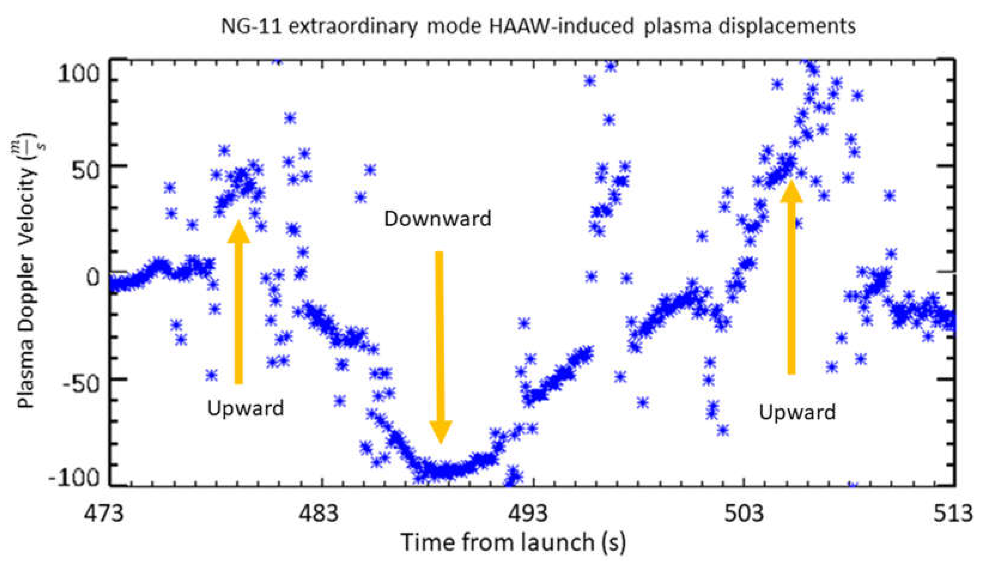
HAAW-induced plasma displacements are observed in the X-mode Doppler velocity plot shown in Figure 2. According to the Dynasonde EDP, the plasma that reflects 4165 kHz O-mode radio waves is near 202 km altitude and the height of the peak plasma density (h’F2) is near 239 km. Based on previous observations [14], rocket-induced HAAW have been found to propagate near the adiabatic speed of sound (Equation (2)) below the F2 layer. Neglecting effects of the increasingly rarefied atmosphere with altitude, the propagation time should be explained by Equation (2) if these plasma displacements are caused by the same HAAW.

Figure 2.
Doppler velocity plot of fixed frequency X-mode observations beginning at 20:54 UTC. Upward and downward plasma displacement peaks are identified.
The altitude the X-mode and O-mode echoes reflect is determined by their radio wave frequencies and the EDP. The plasma frequencies that reflect the X-mode and O-mode radio waves are related by [19]:
where is the X-mode plasma frequency, is the O-mode plasma frequency, and is the electron cyclotron frequency [19]:
Differences in the geomagnetic field between the O-mode and X-mode reflection altitudes are small and the magnetic field value is taken to be the value at 200 km of B = 49.8 μT. Electron charge (e) is in coulombs and electron mass () is in kg.
For a 4165 kHz O-mode plasma frequency (, the corresponding X-mode plasma frequency () is 3394 kHz. According to the EDP, the 3394 kHz plasma is estimated to be near 162 km altitude. The adiabatic sound speed (Equation (2)) computed using temperature values from the NRLMSISE-00 model [20] predicts that it took 80 s for the HAAW to propagate from the 162 km X-mode observation altitude to the 202 km O-mode observation altitude. The O-mode plasma displacements begin at approximately T+553 s and the X-mode plasma displacements begin at approximately T+473 s; it is concluded that the O-mode and X-mode plasma displacements are caused by the same HAAW which propagates vertically near the adiabatic speed of sound. We note that although the HAAW-induced plasma displacements begin 80 s apart, the observation times of the initial upward and downward plasma displacement peaks are separated by 76 s and 86 s, respectively; this suggests that the spatial extent of the HAAW increased as it propagated upward.
3.6. Identification of Multiple Cusp Signatures in Ionograms
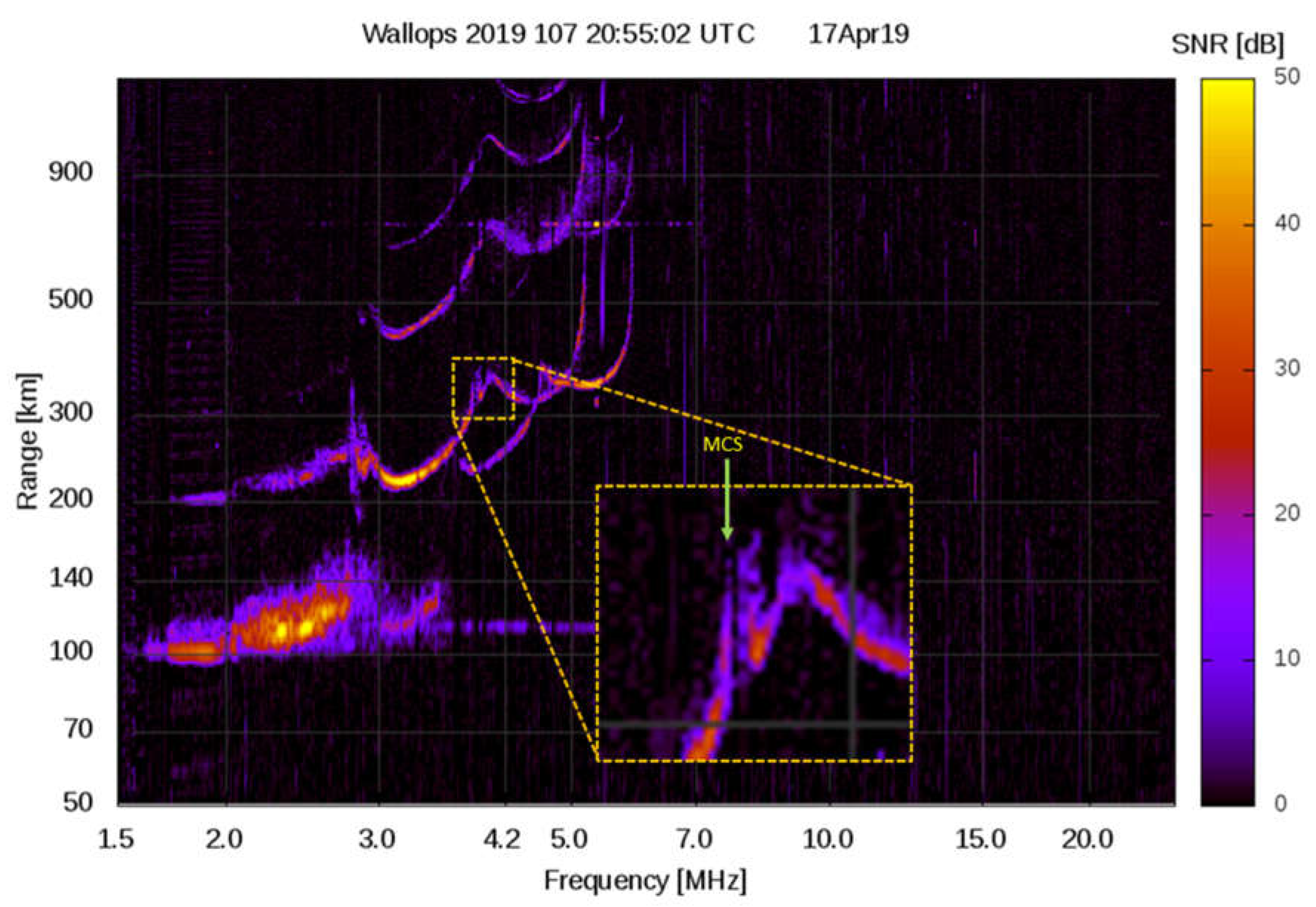
We next determined at what frequency an MCS is most likely to appear in a sweep frequency ionogram, which depends on the HAAW location as a function of time. Using Equation (2), the Dynasonde EDP, and the sounding time of each VIPIR transmit frequency, we determined when the HAAW-induced plasma displacements are co-located with the altitude where the VIPIR sweep frequency radio waves reflect. For the larger amplitude HAAW-induced upward plasma displacement, this co-location occurs at 184 km (4 MHz), 35 s before the HAAW arrives at the 202 km O-mode observation altitude, or 22 s into the 20:55 UTC observation (T+555 s). Figure 3 is the sweep frequency ionogram taken at 20:55 UTC. An additional cusp is clearly visible in the O-mode trace near 4 MHz.
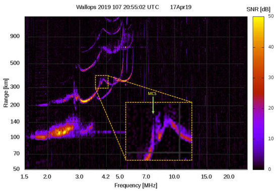
Figure 3.
Sweep frequency ionogram when the NG-11 HAAW arrives at the fixed frequency observation altitude. An MCS is observed in the O-mode trace near 4 MHz.
The same analysis is performed on the X-mode echoes. Eighty seconds prior to the HAAW being observed in the O-mode trace, it should be co-located with the X-mode trace according to Equations (2), (4), and (5). This is the approximate time difference between the corresponding Doppler velocity peaks shown in Figure 1 and Figure 2.
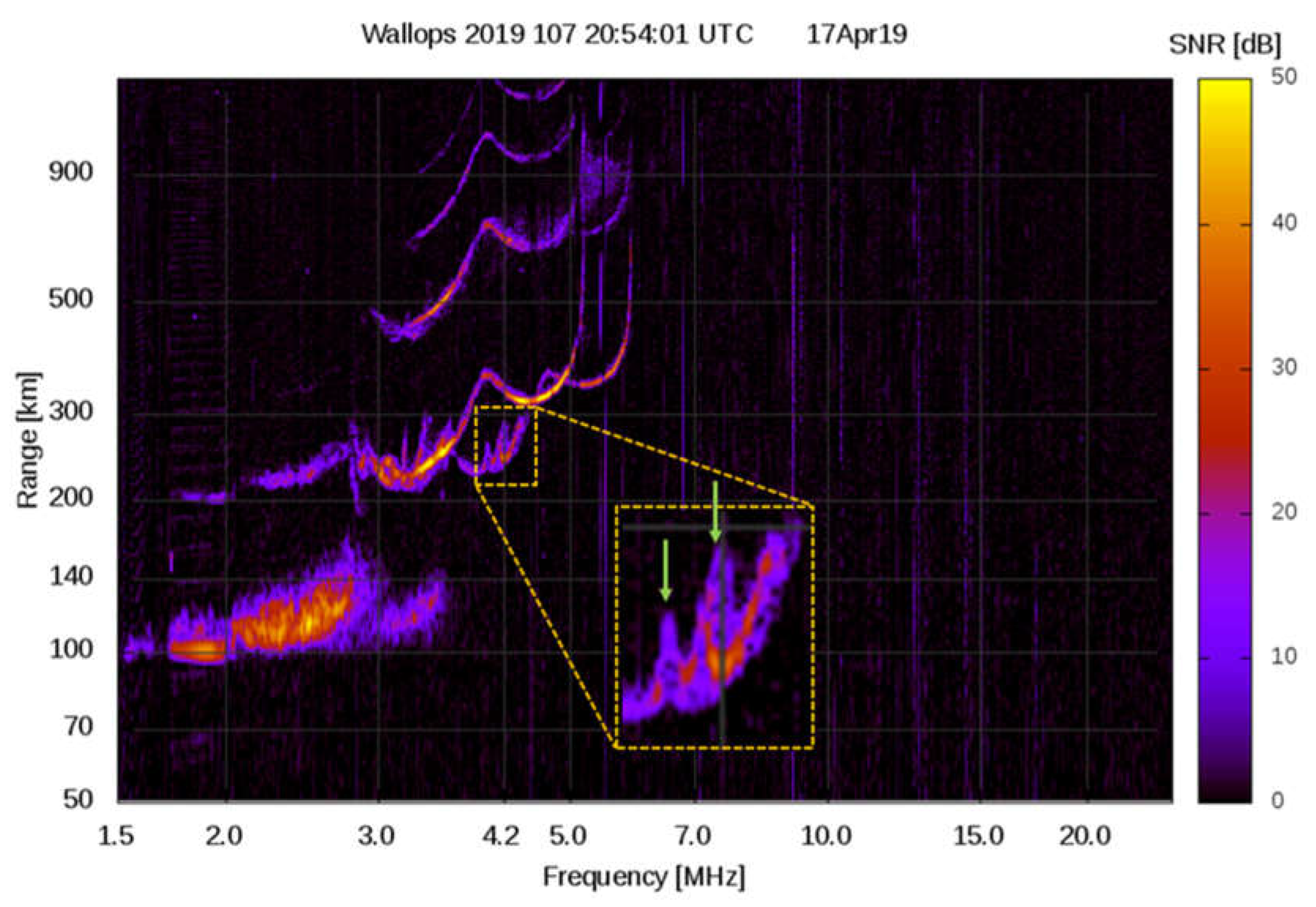
The X-mode trace in the sweep frequency ionogram from 20:54 UTC (Figure 4) is interesting because a pair of MCS exist near 3.9 MHz (where the X-mode radio waves reflect off of the 3.13 MHz plasma at 155 km altitude) and near 4.1 MHz (where the X-mode radio waves reflect off of the 3.33 MHz plasma at 160 km altitude). The VIPIR sounded at 3.9 MHz approximately 21 s (T+494 s) into the observation and at 4.1 MHz approximately 22 s (T+495 s) into the observation.

Figure 4.
Sweep frequency ionogram one minute before the NG-11 HAAW arrives at the fixed frequency observation altitude. A pair of HAAW-induced MCS are present near the 4.2 MHz hash in the X-mode trace.
Using Equation (2), the spatial distance between the two upward plasma displacements in Figure 2 is about 13 km at 162 km altitude. If the two MCS in Figure 4 were caused by the two upward HAAW-induced plasma displacements, the spatial separation should be close to 13 km; the spatial distance between the two MCS in Figure 4 is about 5 km near 160 km altitude, and we conclude that the second MCS in Figure 4 is not caused by the initial upward HAAW-induced plasma displacement.
Table 1 shows that the MCS at the lower frequency in Figure 4 is identified near 155 km altitude (near 3.9 MHz), consistent with the location of the second upward HAAW-induced plasma displacement.
For the second MCS in Figure 4, the radio wave reflection altitude is near 160 km. When this observation is made, the initial HAAW-induced upward plasma displacement is near 170 km altitude and should not affect the radio wave propagation path or range delay. The MCS is closer to the downward HAAW-induced plasma displacements, just above the large amplitude upward HAAW-induced plasma displacements; the MCS is likely caused by a combination of upward and downward plasma displacements near the radio wave reflection altitude.
3.7. Comparison of MCS Range Spread to Changes in Doppler Velocity
Next, we investigated the relative amplitude of the observed MCS range spread in Figure 3 and Figure 4 to the observed Doppler velocity variations identified in Figure 1 and Figure 2.
In Figure 4, the MCS visible at the higher frequency is spread over a greater range than the MCS visible at the lower frequency. That MCS is closer to the height of the peak F1 layer plasma density (h’F1) than the MCS caused by the large amplitude HAAW-induced upward plasma displacement. Both MCS occur below h’F1 and the difference in range spread should be related to their proximity to the layer peak.
In Figure 3, there is only one MCS just below foF1. That MCS corresponds to the larger amplitude upward plasma displacement in Figure 1. The other HAAW-induced plasma displacements are above h’F1 when the frequency sweep is co-located with them, and range deformations that could result in a second MCS are not expected.
3.8. HAAW-Induced Range Variations in Fixed Frequency Ionograms
The location of the HAAW in time was determined, and MCS range deformations were correlated with the larger amplitude HAAW-induced upward Doppler velocity peaks. Next, we investigated range variability in fixed frequency ionograms and compared them to the plasma displacements shown in the Doppler velocity plots in Figure 1 and Figure 2.
Figure 5 is the fixed frequency ionogram from 20:55 UTC, during the same observation when the HAAW-induced MCS is observed in the O-mode trace in the sweep frequency ionogram. There are no apparent range variations associated with the initial upward plasma displacement, but there is an O-mode range decrease that is associated with the downward Doppler velocity peak shown in Figure 1 and an O-mode increase in range associated with the second upward peak in Figure 1. The range increase begins shortly before the observation period ends, and the peak amplitude of the HAAW-induced range delay is not determined.
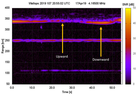
Figure 5.
Fixed frequency ionogram when the NG-11 HAAW arrives at the O-mode fixed frequency observation altitude. Start time is the same as in Figure 1, and arrival times of the initial upward and large amplitude downward plasma displacements are identified as ‘Upward’ and ‘Downward’. The large amplitude upward plasma displacement occurs when the VIPIR is not transmitting, so any effects are not identified.
The fixed frequency ionogram in Figure 6 is from 20:54 UTC, during the same observation when the HAAW-induced MCS is observed in the X-mode trace. This figure shows X-mode range variations associated with both upward Doppler velocity peaks and the downward Doppler velocity peak. The initial upward peak occurs 6 s into the observation, the downward peak occurs 16 s into the observation, and the second upward peak is observed 32 s into the observation. The times correspond to the plasma displacements observed in Figure 2.
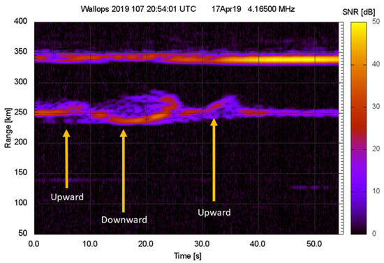
Figure 6.
Fixed frequency ionogram when the NG-11 HAAW arrives at the X-mode fixed frequency observation altitude. Start time is the same as in Figure 2, and arrival times of the initial upward and large amplitude downward and upward plasma displacement peaks are identified as ‘Upward’, ‘Downward’, and ‘Upward’, respectively.
Comparing Figure 2, Figure 3, Figure 4, Figure 5 and Figure 6, the initial upward Doppler velocity peak corresponds to an approximately 20 km increase in range, the downward peak corresponds to an approximately 20 km decrease in range, and the second upward peak corresponds to an approximately 30 km increase in range.
Both the O-mode and X-mode range variations in the fixed frequency ionograms show changes in the range delay associated with the respective Doppler velocity peaks. Range increases are associated with upward Doppler velocity peaks and range decreases are associated with downward Doppler velocity peaks. The amplitude of the O-mode range variations is smaller than the amplitude of the X-mode range variations. This is explained by the proximity of the reflection points to the F1 layer cusp with foF1 near 4 MHz (h’F1 near 192 Km) with the O-mode trace reflecting off of the 4165 kHz plasma and the X-mode trace reflecting off of the 3394 kHz plasma. In Figure 3 and Figure 4, it can be seen that the 4165 kHz plasma is located above h’F1 in the lower F2 region and the 3394 kHz plasma is located below h’F1.
3.9. Comparison to a Previous Observation
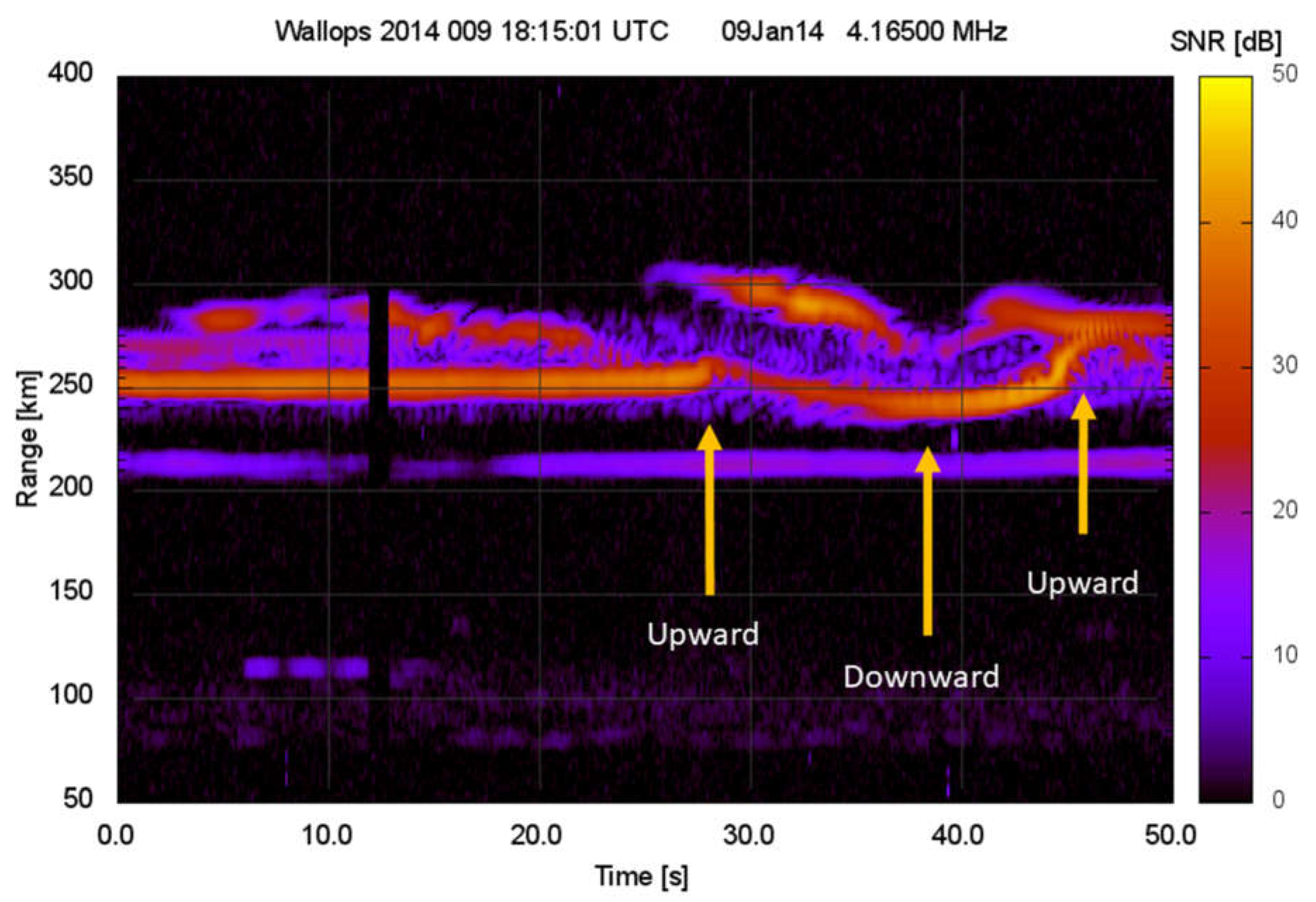
Similar range variations were observed during an earlier rocket launch. The ORB-1 rocket launched from WFF on 9 January 2014 at 18:07 UTC (13:07 EST). During that experiment, HAAW-induced plasma displacements were observed at the 4165 kHz fixed frequency just below h’F1. The Doppler velocity and range variations were amplified significantly by cusp effects [14].
The fixed frequency ionogram from the ORB-1 observations (Figure 7) shows features similar to those seen in Figure 6. When these observations were made, the 4165 kHz O-mode echoes reflected just below h’F1, similar to the X-mode plasma during the NG-11 flight. During the ORB-1 flight, the HAAW passed through the fixed frequency observation altitude after the VIPIR had already swept past foF1. Consequently, the HAAW was located in the bottom side F2 region when the frequency sweep passed the co-located plasma, and there was no significant increase in the range delay and no MCS was observed in the sweep frequency ionogram.

Figure 7.
Fixed frequency ionogram when ORB-1 HAAW arrives at the fixed frequency O-mode observation altitude. Arrival times of the initial upward and large amplitude downward and upward plasma displacements are marked ‘Upward’, Downward’, and ‘Upward’, respectively.
4. Discussion
We have investigated the relationship between MCS in sweep frequency ionograms, range variations in fixed frequency ionograms, and fixed frequency Doppler velocity variations. Previous observations of MCS have been limited to deformations in traditional sweep frequency ionograms. For the first time, we correlate observed HAAW-induced plasma displacements with the MCS, and we validate a previously proposed explanation for how and why MCS form.
A motivation of this continuing research is to understand how a HAAW displaces ionospheric plasma and how those plasma displacements result in features that have been observed in ionograms. These results could help answer several important questions including: how is radio wave propagation affected by HAAW-induced plasma displacements [16]; should HAAW energy transport be included into global atmospheric models [22]; and can we explain previous HAAW observations made using traditional ionosondes [1], GNSS [23], and other instruments.
The presented results are intended to advance our understanding of how HAAW-induced atmospheric disturbances manifest in remote sensing observations. Understanding what is seen in the observations is needed to help specify the physics of the HAAW overpressure anomaly and how the atmosphere responds to it. Understanding the physics of the HAAW overpressure anomaly and how the atmosphere responds to it is needed to understand how infrasonic waves are related to weather, climate, and extreme events.
Three investigations that could enhance the results presented in this article are not included. These include determination of the HAAW vertical propagation velocity, specification of the overpressure anomaly, and the production of synthetic ionograms. All three of these would require a significant application of theory, detracting from the main purpose of this article, which is to present experimental results. Also, these investigations are not trivial, and each deserves its own dedicated treatment.
In this article, the location of the HAAW has been measured at several altitudes using sweep and fixed frequency data in both O-mode and X-mode echoes. Previously, HAAW have been observed to propagate faster than the adiabatic speed of sound in the thermosphere [21]. The presented results show the HAAW propagation velocity is close to the adiabatic speed of sound, suggesting the observations are made at a low enough altitude that effects of the rarefied atmosphere did not have to be considered.
A theoretical investigation of how Equation (2) fails, compared to observational results, is needed so this observation method can be used to determine the composition and temperature of the thermosphere. This has potentially important implications for model validation and satellite drag in low earth orbit.
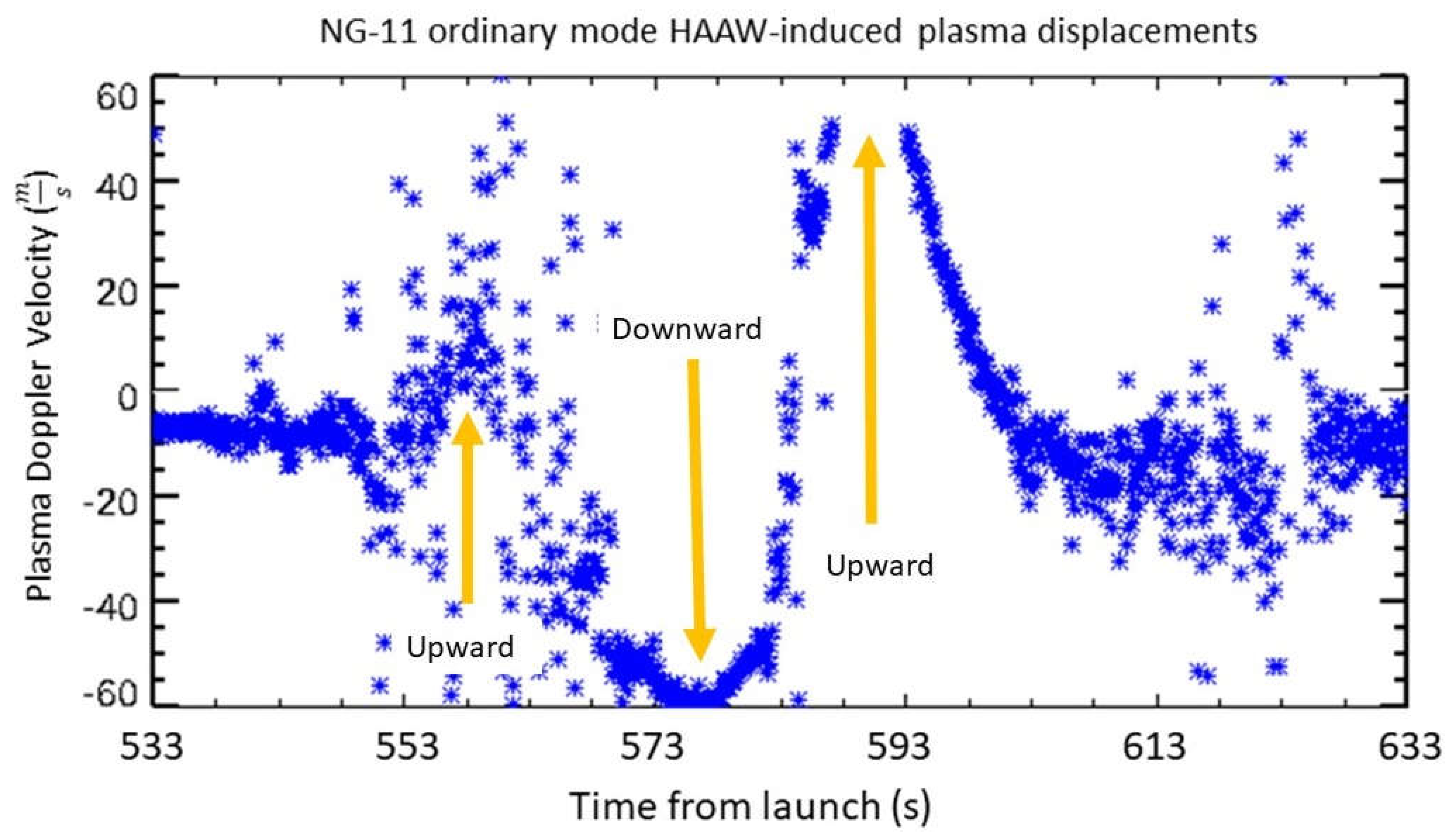
Specification of the physics of the overpressure anomaly has important implications in the understanding of atmospheric dynamics and energy transfer. In Figure 1 and Figure 2, HAAW-induced Doppler velocities are shown. To first order, the rate of change of these velocity values should correspond to the form of the HAAW-induced pressure gradient force. Specifically, an initial upward displacement followed by a downward displacement is what would be expected from a simple overpressure anomaly; the following upward displacement could be the result of a return of displaced electrons to equilibrium. These are characteristic of a self-reinforcing wave that approximately maintains its shape as it propagates in the thermosphere.
Rocket engines produce a complex acoustic signature that does not resemble a simple overpressure anomaly. Determination of the form of the pressure anomaly is important toward understanding what portions of the acoustic waves are attenuated in what regions of the atmosphere, and how the wave structure converges as it propagates. Within the scope of the presented results, we have shown that the presented Doppler velocity values include effects of HAAW-induced changes in the index of refraction. Obtaining real velocity values is not trivial, and a careful investigation of how the presented results can be used to determine the form of the overpressure anomaly is needed.
A final investigation that is omitted is the comparison of synthetic ionograms to the experimental results, similar to what was done by Maruyama et al. (2011) [1] and Maruyama and Shinagawa (2013) [3]. To create physically realistic synthetic ionograms that contain MCS, Equation (1) requires the presence of a local electron density peak. An ionosonde can only measure an increasing EDP, and the presence of a local electron density peak has to be inferred or determined through the application of theory. The scope of this article is limited to experimental results, which could generate synthetic ionograms that do not infer local density peaks, but those synthetic ionograms could only produce HAAW-induced ionogram deformations and not MCS.
There are two other problems with using the presented results to generate synthetic ionograms to try and reproduce the MCS. The first problem is that introducing local electron density peaks would be trivial because any local electron density peak should result in a cusp according to Equation (1). The second problem is that we would have to account for the plasma displacements shown in Figure 1 and Figure 2, which would make the EDP near the reflection point change rapidly and would have to include spatial variations smaller than the spatial resolution of the Dynasonde EDP. That means small scale structure in the ionosphere would be neglected while considering HAAW-induced structure on those same spatial scales. These considerations make it impossible to compute the real range delay, and the results would be unreliable.
5. Conclusions
This article presents the first observations of MCS in ionograms after an Antares rocket launch. These observations were made using an experimental method invented by the authors which has been used to observe Doppler velocity and range variations in ionospheric plasma. The results allow for a detailed comparison between observed Doppler velocity variations and ionogram deformations, including the MCS.
The MCS in the presented ionograms appear in the form of additional cusps. The formation of cusps near a plasma layer peak is predicted by the Appleton-Hartree equation as a consequence of the increasing slope of the EDP near a layer peak, and the resulting refractive index. These MCS manifest as a result of the echo range delay caused by changes in the radio wave propagation velocity and path.
During the NG-11 experiment, HAAW-induced Doppler velocity variations were observed in both the O-mode and X-mode fixed frequency echoes. Both traces were separated in range and time and could be analyzed individually. For both traces, plasma displacements were observed with a high time resolution of 80 ms as the HAAW passed through the observed plasma.
The MCS were observed in both O-mode and X-mode echoes in sweep frequency ionograms. The combination of timing and atmospheric conditions needed to observe HAAW-induced MCS in both the O-mode and X-mode traces is unexpected, and would not be possible for common ionosonde sounding intervals of 5 to 15 min or for measurement modes which take several minutes to complete an ionogram. The design and construction of the Wallops VIPIR is the instrumentation technology that enables the rapid measurement modes necessary for these discoveries [15].
HAAW-induced range variations are apparent in the fixed frequency ionograms. This provides an additional validation of the connection between the observed Doppler velocity variations and the MCS identified in the sweep frequency ionograms. The range and Doppler velocity variations are observed simultaneously and establish the relationship between plasma displacements and the range delay.
Making use of the experimental modes of the VIPIR, the instrument functions effectively as both a Dynasonde [18,21] and as a fixed frequency Doppler sounder [24]. This has allowed for the direct correlation of two independent data sets and an improved understanding of how a HAAW displaces ionospheric plasma and causes deformations in ionograms.
Author Contributions
All authors contributed to all aspects of this research and manuscript preparation. All authors have read and agreed to the published version of the manuscript.
Funding
This research was funded by NASA project Daytime Lower Ionosphere Dynamo Experiment, grant number 80NSSC20K0756 and by the NOAA Cooperative Agreement with CIRES, NA17OAR4320101.
Institutional Review Board Statement
Not applicable.
Informed Consent Statement
Not applicable.
Data Availability Statement
Data used in support of this work can be obtained from the NOAA National Centers for Environmental Information, https://www.ncei.noaa.gov/ (accessed on 5 May 2022).
Acknowledgments
The authors thank NASA Wallops Flight Facility for their ongoing support.
Conflicts of Interest
The authors declare no conflict of interest.
References
- Maruyama, T.; Tsugawa, T.; Kato, H.; Saito, A.; Otsuka, Y.; Nishioka, M. Ionospheric multiple stratifications and irregularities induced by the 2011 off the Pacific coast of Tohoku Earthquake. Earth Planets Space 2011, 63, 869–873. [Google Scholar] [CrossRef]
- Maruyama, T.; Tsugawa, T.; Kato, H.; Ishii, M.; Nishioka, M. Rayleigh wave signature in ionograms induced by strong earthquakes. J. Geophys. Res. 2012, 117, A08306. [Google Scholar] [CrossRef]
- Maruyama, T.; Shinagawa, H. Infrasonic sounds excited by seismic waves of the 2011 Tohoku-oki earthquake as visualized in ionograms. J. Geophys. Res. Space Phys. 2013, 119, 4094–4108. [Google Scholar] [CrossRef]
- Maruyama, T.; Yusupov, K.; Akchurin, A. Ionosonde tracking of infrasound wavefronts in the thermosphere launched by seismic waves after the 2010 M8.8 Chile earthquake. J. Geophys. Res. 2016, 121, 2683–2692. [Google Scholar] [CrossRef]
- Maruyama, T.; Yusupov, K.; Akchurin, A. Interpretation of deformed ionograms induced by vertical ground motion of seismic Rayleigh waves and infrasound in the thermosphere. Ann. Geophys. 2016, 34, 271–278. [Google Scholar] [CrossRef]
- Astafyeva, E. Ionospheric detection of natural hazards. Rev. Geophys. 2019, 57, 1265–1288. [Google Scholar] [CrossRef]
- Mabie, J. Infrasound induced plasma perturbations associated with geomagnetic pulsations. Russ. J. Earth Sci. 2019, 19, ES3002. [Google Scholar] [CrossRef]
- Toshihiko, I.; Nose, M.; Han, D.; Gao, Y.; Hashizume, M.; Choosakul, N.; Sinagawa, H.; Tanaka, Y.; Utsugi, M.; Saito, A.; et al. Geomagnetic pulsations caused by the Sumatra earthquake on December 26, 2004. Geophys. Res. Lett. 2005, 32, L20807. [Google Scholar] [CrossRef]
- Kakinami, Y.; Kamogawa, M.; Tanioka, Y.; Watanabe, S.; Gusman, A.R.; Liu, J.; Watanabe, Y.; Mogi, T. Tsunamigenic ionospheric hole. Geophys. Res. Lett. 2012, 39, L00G27. [Google Scholar] [CrossRef]
- Saito, A.; Tsugawa, T.; Otsuka, Y.; Nishioka, M.; Iyemori, T.; Matsumura, M.; Saito, S.; Chen, C.H.; Goi, Y.; Choosakul, N. Acoustic resonance and plasma depletion detected by GPS total electron content observation after the 2011 off the Pacific coast of Tohoku earthquake. Earth Planets Space 2011, 63, 64. [Google Scholar] [CrossRef]
- Zettergren, M.D.; Snively, J.B. Ionospheric signatures of acoustic waves generated by transient tropospheric forcing. Geophys. Res. Lett. 2013, 40, 5345–5349. [Google Scholar] [CrossRef]
- Daniels, F.B.; Siegfried, J.B.; Harris, A.K. Vertically traveling shock waves in the ionosphere. J. Geophys. Res. 1960, 65, 1848–1850. [Google Scholar] [CrossRef]
- Davies, K.; Baker, D.M. Ionospheric Effects Observed around the Time of the Alaskan Earthquake of March 28, 1964. J. Geophys. Rev. 1965, 70, 2251–2253. [Google Scholar] [CrossRef]
- Mabie, J.; Bullett, T.; Moore, P.; Vieira, G. Identification of rocket-induced acoustic waves in the ionosphere. Geophys. Res. Lett. 2016, 32, 43. [Google Scholar] [CrossRef]
- Grubb, R.N.; Livingston, R.; Bullett, T.W. A New General Purpose High Performance HF Radar. In Proceedings of the URSI General Assembly. 2008. Available online: https://www.ursi.org/proceedings/procGA08/papers/GHp4.pdf (accessed on 1 June 2014).
- Mabie, J.; Bullett, T. Infrasonic wave induced variations of ionospheric HF sounding echoes. Rad. Sci. 2019, 54, 876–887. [Google Scholar] [CrossRef]
- Zabotin, N.A.; Wright, J.W.; Zhbankov, G.A. NeXtYZ: Three-dimensional electron density inversion for dynasonde ionograms. Radio Sci. 2006, 41, 6. [Google Scholar] [CrossRef]
- Wright, J.W. Ionogram inversion for a tilted ionosphere. Radio Sci. 1990, 26, 1175–1182. [Google Scholar] [CrossRef]
- Davies, K. Ionospheric Radio Propagation; Central Ratio Propagation Laboratory Library of Congress Catalog Card Number: 64-60061; United States Department of Commerce National Bureau of Standards: Washington, DC, USA, 1965.
- Pederick, L.H.; Cervera, M.A. Semiempirical model for ionospheric absorption based on the NRLMSISE-00 atmospheric model. Rad. Sci. 2014, 49, 81–93. [Google Scholar] [CrossRef]
- Mabie, J. Rocket Induced High Altitude Acoustic Waves; ProQuest Dissertations and Theses: Ann Arbor, MI, USA, 2019; ISBN 9781392642719. [Google Scholar]
- Akmaev, R.A. Whole Atmosphere Modeling: Connecting Terrestrial and Space Weather. Rev. Geophys. 2011, 49, 4. [Google Scholar] [CrossRef]
- Zettergren, M.D.; Snively, J.B.; Komjathy, A.; Verkhoglyadova, O.P. Nonlinear ionospheric responses to large-amplitude infrasonic-acoustic waves generated by undersea earthquakes. J. Geophys. Res. Space Phys. 2017, 122, 2272–2291. [Google Scholar] [CrossRef]
- Lastovicka, J.; Chum, J. A review of the results of the international ionospheric Doppler sounder network. Adv. Space Res. 2017, 60, 1629–1643. [Google Scholar] [CrossRef]


Publisher’s Note: MDPI stays neutral with regard to jurisdictional claims in published maps and institutional affiliations. |
© 2022 by the authors. Licensee MDPI, Basel, Switzerland. This article is an open access article distributed under the terms and conditions of the Creative Commons Attribution (CC BY) license (https://creativecommons.org/licenses/by/4.0/).