Article

Impact of Collaborative Agglomeration of Manufacturing and Producer Services on Air Quality: Evidence from the Emission Reduction of PM2.5, NOx and SO2 in China

1
Hainan Open Economy Research Institute, School of Economics, Hainan University, Haikou 570228, China
2
School of Business Administration, Zhongnan University of Economics and Law, Wuhan 430073, China
*
Author to whom correspondence should be addressed.
Atmosphere 2022, 13(6), 966; https://doi.org/10.3390/atmos13060966
Submission received: 13 May 2022 / Revised: 6 June 2022 / Accepted: 11 June 2022 / Published: 14 June 2022

Abstract

:
Industrial agglomeration is a major source of regional economic development and the main pattern enterprises employ after having developed to a certain stage. Industrial agglomeration also affects the emissions of air pollutants in production. Based on provincial panel data for China from 2006 to 2019, this paper introduces the full generalized least squares (FGLS) panel econometrics model. By considering spatial correlation, the potential endogenous problem has been controlled using the instrumental variable and the effects of the co-agglomeration of manufacturing and producer services on three major air pollutants, i.e., SO2, PM2.5, and NOx, have been empirically estimated. The empirical results show that: (1) The agglomeration of manufacturing increases the emission of PM2.5 in the air, while the agglomeration of producer services and the co-agglomeration of manufacturing and producer services reduce it. Moran correlation index test showed that SO2 and NOx had no significant spatial correlation. (2) The agglomeration of manufacturing, the agglomeration of producer services, and co-agglomeration exert the most significant effects on PM2.5 in the air in central and western China. This is probably because of the availability of basic natural resources in these areas. (3) The energy consumption structure mediates the effect of the agglomeration of manufacturing on PM2.5, and human capital mediates the effect of the agglomeration of producer services on PM2.5 emissions. Based on the results, policy suggestions to improve the atmospheric environment during the process of industrial agglomeration are proposed.

1. Introduction

1.1. Background

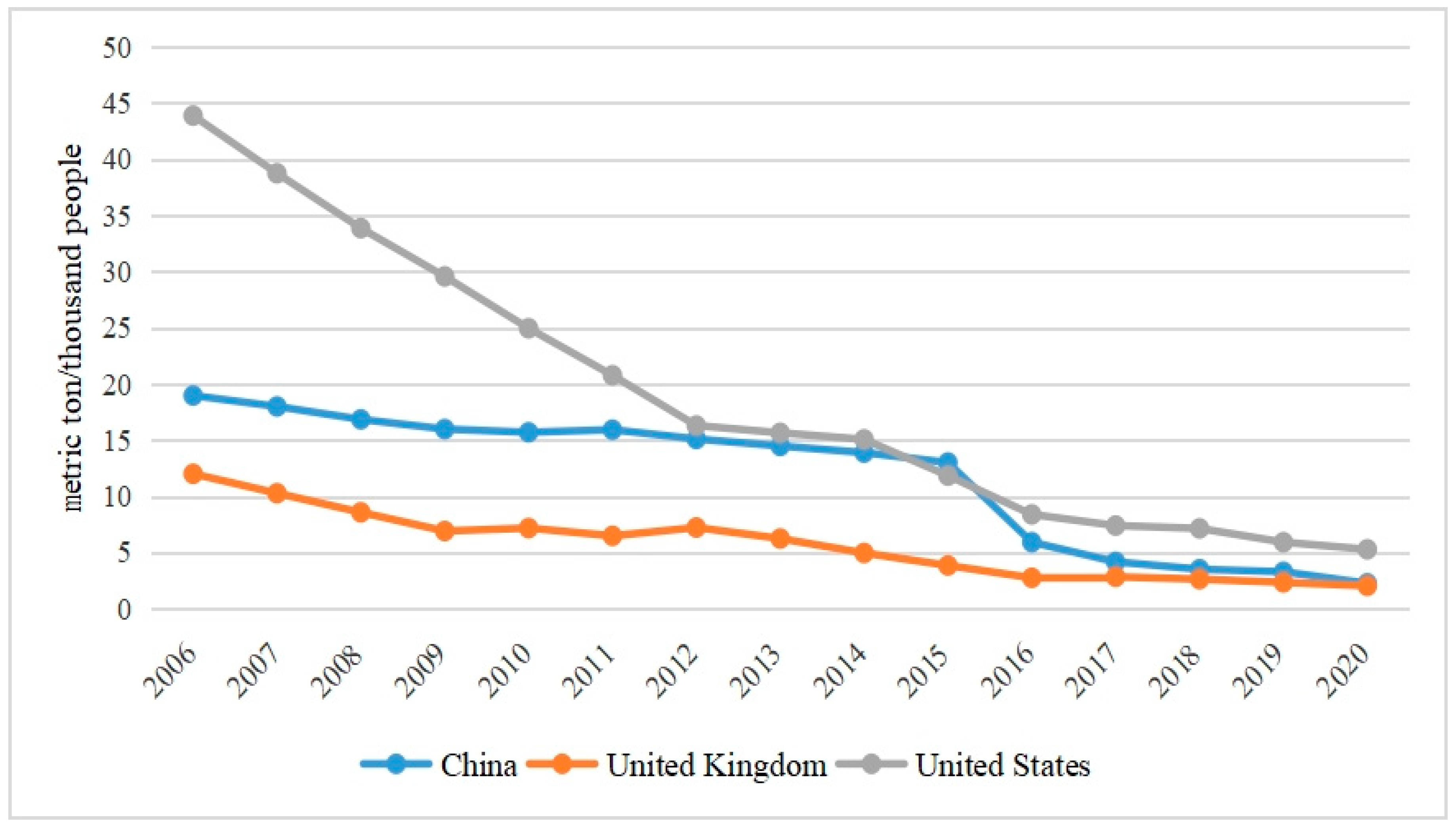
The relationship between economic growth and environmental pollution has long been a research priority for many scholars [1,2]. Since reform and opening-up, China has achieved rapid economic development, where China’s manufacturing industry (a pillar industry of economic development) and service industry (the tertiary industry) have expanded rapidly in scale. Manufacturing enterprises consume considerable fossil, petroleum, and other energy sources in the production process, where the combustion of these energies generates numerous air pollutants [1,3,4]. Moreover, this massive pollution discharge by enterprises during production also impacts the physical health and daily life of nearby residents [5,6]. Compared with manufacturing, the service industry better satisfies the demands of sustainable economic development. According to the China Ecological Environment Status Bulletin in 2020, 202 (59.9%) of all 337 Chinese cities met the proposed standards on ambient air quality. Days where PM2.5 was the major pollutant accounted for most of the number of days when air quality did not meet the standards [7,8,9]. As a result of intensified air pollution, respiratory tract infections and other associated diseases have also presented an increasing trend among residents. President Xi has proposed that “Lucid waters and lush mountains are invaluable assets.” In this spirit, the effective control and governance of air pollution constitute the basis for guaranteeing sustainable economic development and safeguarding people’s physical health. In this sense, it has become necessary to adjust economic development policies and the overall industrial layout and improve the ecological environment, thus achieving high-quality economic development. Currently, as countries around the world pay more attention to the management of the air environment, they are beginning to see the results of their efforts in the management of air pollution. Figure 1, Figure 2 and Figure 3 show diagrams of the emissions of PM2.5, SO2, and NOx in China, the UK, and the US. Figure 1, Figure 2 and Figure 3 show that the decreasing trend of SO2 and NOx in China, the UK, and the US is significant, especially since the decreasing trend of per capita emissions in China is faster than that of the UK and the US. This indicates that China has made great progress in air pollution reduction. At the same time, the mean annual exposure (μg/m3) of PM2.5 in China is much higher than that of the UK and the US, despite the significant downward trend, which further indicates that we need to optimize the industrial structure and use renewable energy to improve air quality.
Air pollution has the dual characteristics of spatial agglomeration and diffusion. The number of agglomerated industrial enterprises affects the air quality of both local and adjacent areas. To a certain extent, a regional link exists between air pollution and industrial agglomeration, making it highly necessary to clarify their relationship [10,11,12,13]. The effect of industrial agglomeration on air pollution is mainly embodied in the following two aspects: (1) Industrial agglomeration aggravates local air pollution: The large-scale agglomeration of enterprises, especially industrial enterprises, generates industrial waste gases and wastewater and increases the emissions of PM2.5, SO2, NOx and other air pollutants in areas of industrial agglomeration. If the local government blindly pursues rapid economic development, the difficulty of regional environmental governance will be further exacerbated, resulting in further environmental deterioration. In addition, the agglomeration of enterprises also attracts the settlement of employees in areas close to plants, and pollution discharge by residents also aggravates local environmental pollution [14,15,16]. (2) Industrial agglomeration mitigates local air pollution, mainly by reducing the emissions of air pollutants through economies of scale, technology spillover, production efficiency, and intermediate sharing mechanisms [17,18]. On the one hand, the economies of scale effect induced by industrial agglomeration can lower enterprises’ production costs. Relying on advanced production technologies in agglomeration areas, enterprises can increase production efficiency, transform production modes, and promote energy conservation and emission reduction, thus effectively alleviating emissions of harmful gases. From the perspective of regional innovation, both specialized agglomeration and diversified agglomeration can promote regional innovation, but the former has a more apparent spillover innovation effect [19,20,21]. On the other hand, industrial agglomeration can provide the diversified intermediate services required by regional development, so that the economies of scale effect can be achieved in manufacturing through the sharing of intermediate services [22]. In particular, intermediate services provided in a concentrated manner by producer services (represented by finance, law, logistics, etc.) save time and economic costs borne by enterprises when searching for intermediate service providers. Consequently, they can invest more funds and energy in conducting R&D, improving production conditions, and promoting sustainable production.
This paper mainly explores the mechanism underlying the effect industrial agglomeration has on air pollution from the following three aspects: the agglomeration of manufacturing, the agglomeration of producer services, and the co-agglomeration of manufacturing and producer services. To be specific, industrial waste gases and wastewater generated by traditional manufacturing, mainly because of the utilized production links and modes, deteriorate the local environment [23,24,25,26]. However, the economies of scale effect produced by industrial agglomeration may drive enterprises to increase their production efficiency and adopt green energies, thus weakening the impact of industrial pollution on the local environment [23,24,25,26]. Emerging producer services mainly serve manufacturing enterprises and consume very little energy. Combined with the use of clean energies, they can effectively mitigate air pollution in agglomeration areas [10,13]. By virtue of inter-industry knowledge overlap and technology spillover, co-agglomeration of industries yields a collaborative symbiosis effect, which can upgrade interregional industrial structures, transform enterprise production modes, and further optimize interregional air quality.

1.2. Literature Review

Scholars have extensively studied the relationships between economic growth, industrial agglomeration, and air pollution [27,28]. Their main points of view are summarized in the following: (1) The “Environmental Kuznets Curve hypothesis” basically states that, as a result of rapid economic development in a country, the environmental quality of the country presents a deteriorating trend first and an improving trend afterward [29,30,31,32,33]. Scholars advocating the “Environmental Kuznets Curve hypothesis” unfold their research mainly from the perspective of carbon dioxide emissions. Carbon dioxide and per capita GDP both present U-shaped, N-shaped, and monotonically increasing relationships, which validate the “Environmental Kuznets Curve hypothesis” [8,34,35]. (2) Industrial agglomeration aggravates air pollution. Scholars unfolding their research from this perspective mainly focus on energy consumption and environmental governance costs of the agglomeration of manufacturing using the “Pollution Haven hypothesis”. In the agglomeration process of manufacturing enterprises, the combustion of energy sources by many industrial enterprises increases the emissions of air pollutants, resulting in the deterioration of air quality [16,34]. A large number of enterprises in agglomeration areas further increase the difficulty of environmental pollution governance. Most enterprises have adopted a “free-ride” economies of scale approach and are reluctant to pay the transaction costs incurred by diseconomies of scale. The “Pollution Haven hypothesis” also partially explains the environmental pollution caused by the agglomeration of manufacturing industries [36,37]. That is, countries facing high costs of environmental regulation tend to transfer their manufacturing to countries with low costs of environmental regulation. Consequently, developing countries can increase their manufacturing yield through the absorption of foreign capital, but must still face the increasing emissions of harmful air pollutants [17]. (3) Industrial agglomeration mitigates air pollution. Scholars supporting this perspective argue that industrial agglomeration improves production efficiency, innovation level, production mode transformation, and environmental regulation of enterprises [36,37,38]. They further argue that knowledge and technology spillover effects produced by agglomeration can raise the technical level of enterprises, thus driving them to develop environmentally friendly production equipment, transform production modes, and lower air pollution levels [39]. To encourage economic development and attract enterprises, the government may choose to uniformly purchase pollution discharge facilities in an agglomeration area, thus removing the costs of pollution discharge facilities for individual enterprises. Benefiting from raised regional agglomeration levels and improved production conditions, enterprises can invest more funds in governing pollution discharge, thus mitigating air pollution [40]. The adoption of new energies and technologies by enterprises can also make their production processes greener and more environmentally friendly, thus contributing to the improvement of local air quality [41]. To improve residents’ living environment, the government may introduce strict environmental regulation policies. Zhou and Feng (2017) [42] showed that environmental regulation can significantly inhibit the expansion of heavy industries and reduce the use of fossil energy sources, further showing that there is a significant negative relationship between environmental regulation and the emission of air pollutants.

1.3. Hypotheses and Theoretical Mechanisms

1.3.1. Hypotheses

In terms of the agglomeration of manufacturing, in this paper, the mechanism underlying the effect of the agglomeration of manufacturing on air pollution is clarified from two perspectives. Then, how the agglomeration of manufacturing increases the emissions of interregional air pollutants is analyzed. On the one hand, this is because of the use of excessive non-clean energies by many agglomerated manufacturing enterprises. Manufacturing generally refers to traditional energy-intensive industries. Industrial production can increase regional industrial added value and quickly raise the local economic development level. During the early stages of the reform and opening up, local governments often sacrificed the environment for economic growth by excessively burning traditional energy sources such as coal and oil in industrial production. This continually increased the emissions of SO2, NOx, PM2.5, and PM10 into the air [10,11,18]. On the other hand, when excessive industrial pollution discharge by enterprises in the agglomeration process was complicated by the expansion of the regional population and a substantial increase in the number of enterprises in the initial stage of agglomeration, the emissions of regional air pollutants increased abruptly [2,12,43]. Compelled by the competition effect induced by massive agglomeration, enterprises attach great importance to new product R&D for the sake of market share, while commonly neglecting the addition and replacement of basic pollution discharge facilities. Consequently, industrial pollution discharge adversely impacts the daily living environment of nearby residents. Based on the above analysis, the first hypothesis is proposed.
Hypothesis 1 (H1).
Massive agglomeration of manufacturing enterprises increases energy consumption, industrial pollution discharge, and air pollutant emissions in agglomeration areas.
Producer services differ from manufacturing, as producer services mainly serve manufacture and can be regarded as intermediate service providers of manufacturing. The production process is cleaner under the agglomeration of producer services. The massive agglomeration of producer service enterprises creates the economies of scale effect, which reduces the transaction costs of producer services. In this way, enterprises can invest more funds in improving the producer service level as well as intermediate product production and provide more energy-conserving and environment-friendly intermediate products for manufacturing. This effectively reduces the emissions of regional air pollutants [13,44]. Enterprises engaged in producer services are largely based on personnel and services. While such enterprises generate certain waste gases and wastewater in the production process, they consume very few energy-intensive resources. Therefore, increasing the number of producer service enterprises can, to a certain extent, mitigate regional air pollution. Based on this, the second hypothesis is presented.
Hypothesis 2 (H2).
By virtue of their production features, producer services can effectively inhibit the emissions of regional air pollutants.
The co-agglomeration of industries creates a spatial spillover effect, which can drive local enterprises and enterprises in adjacent areas to share resources (such as knowledge, technology, and labor), learn from each other, transform production modes, and increase interregional production efficiency. When the local government renews the pollution discharge facilities of the region or introduces strict environmental regulation policies, the local governments of adjacent areas will be affected, which further changes the conditions of interregional environmental regulation [45]. The study by Thiel et al. (2016) [46] has indicated that environmental regulation can significantly inhibit environmental pollution, high environmental pressure prompts enterprises to upgrade their R&D and technologies, and more efficient utilization and treatment of pollutants lead to less serious environmental pollution. Moreover, the co-agglomeration of industries also creates a collaborative symbiosis effect, which can realize complementary production between enterprises, optimize internal and external production structures, and effectively reduce the emissions of interregional air pollutants. In this context, the third hypothesis is put forward.
Hypothesis 3 (H3).
The collaborative symbiosis, circular economy, and other effects created by the co-agglomeration of manufacturing and producer services mitigate regional air pollution.

1.3.2. Theoretical Mechanisms

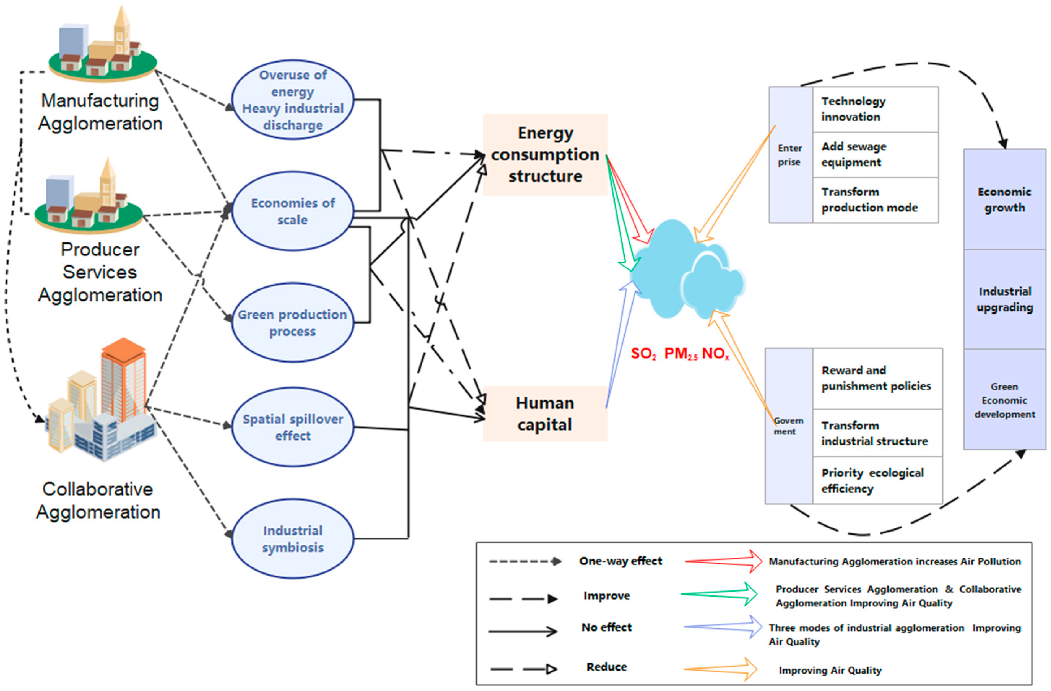
Industrial agglomeration may also indirectly affect air pollution through mediating factors. The environmental regulation intensity of a region directly influences the local pollution governance level. Strict environmental regulation not only encourages the adjustment of the energy structure and the transformation of production modes in the region, but also urges enterprises to recruit R&D personnel, conduct scientific and technological innovation, and increase labor productivity [8,29,37]. Considering this, this paper starts with regional energy consumption structure and human capital to analyze the factors that mediate the effect of industrial agglomeration on air pollution, and Figure 4 depicts the route map of these agglomerations.
Regarding the energy consumption structure, the consumption and combustion of coal by a region directly affect the environmental quality of that region. The industrial waste gases generated in large amounts by coal combustion increase the emissions of PM2.5 and SO2 into the air. Considering that a massive agglomeration of enterprises also directly affects regional coal consumption, in this paper the proportion of regional coal consumption in total regional energy consumption is adopted to measure whether industrial agglomeration affects regional air pollution through the energy consumption structure. Regarding human capital, agglomeration creates a labor pool effect, which enables local enterprises to share abundant labor resources and lays the foundation of local human capital. With the introduction of increasingly refined environmental policies by the government, it becomes imperative for enterprises to fulfill their heavy responsibilities of energy conservation and emission reduction by adopting new energies or by transforming production modes. To do so, they must intensify R&D investment, recruit sufficient R&D personnel, conduct scientific and technological innovation, increase production efficiency, and transform production modes. Therefore, human capital is adopted as a further mediating variable and its role between agglomeration and air pollution is discussed.

2. Data Sources

2.1. Setup of Econometric Model

The relationship between environmental pollution and human activities has been extensively studied for a considerable time. It was first studied by the US economists Ehrlic et al. (1972) [47], who used the equation I = PE. Later, Rosa et al. (1998) [48] introduced elasticity coefficients into the model and modified it into the more practical STIRPAT model which also considers the effects of changes in various scenarios. The specific equation is as follows:
I = a P b A C T d e
where I, P, A, and T denote pollution degree, population scale, per capita wealth, and technical level, respectively. a is a constant term, b, c, and d are elasticity coefficients, and e is an error term.
By logarithmizing both sides of Equation (1), Equation (2) is obtained:
l n I = l n a + b l n P + c l n A + d l n T + ε
where a is a constant term, b, c, and d are the parameters to be estimated, and ε is an error term. The agglomeration indices of different industries are added based on the study by Rosa et al. (1998) [48]. The continuous variables in these models (I, a, P, A, and T) are taken from the common logarithm, which can unify the dimensionless parameters, and reduce the heteroscedasticity by minimizing the influence of the outliers [49]. The econometrics model of this paper is set up as follows:
l n P o l l u t i o n i t = α 0 + α 1 l n a g g i t + α 2 X i t + λ i t + ε i t
where i denotes the province, t denotes the year, P o l l u t i o n i t denotes air pollution indices, including PM2.5, NOx, and SO2; agg denotes the core explanatory variables of agglomeration, including the agglomeration of manufacturing (Magg), the agglomeration of producer services (Sagg), and the co-agglomeration of manufacturing and producer services (Cagg); α 0 is a constant term, α 1 is a parameter to be estimated, λ i t represents time and individual fixed effects, and ε i t is a stochastic disturbance term.

2.2. Core variables

2.2.1. Explained Variables

This paper explores the effect of industrial agglomeration on three major air pollution sources, i.e., SO2, PM2.5, and NOx, which constitute the main explained variables of this paper. Among them, PM2.5 is defined as the haze index of each province each year, which is mainly explained by the annual mean concentration; NOx is defined as the oxynitride emission of each province each year (10,000 tons), and SO2 is defined as the sulfur dioxide emission in waste gases of each province each year (10,000 tons).
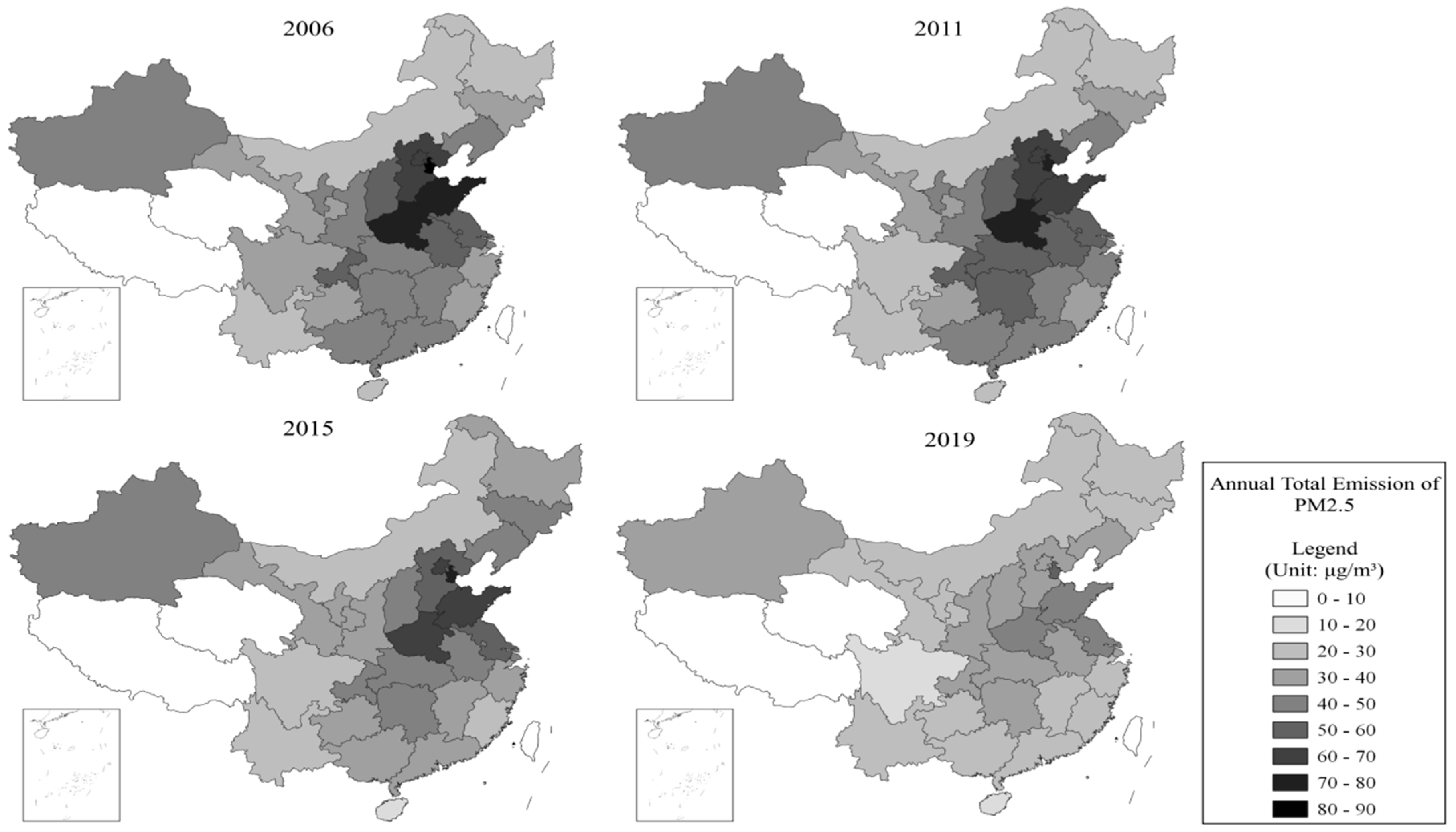
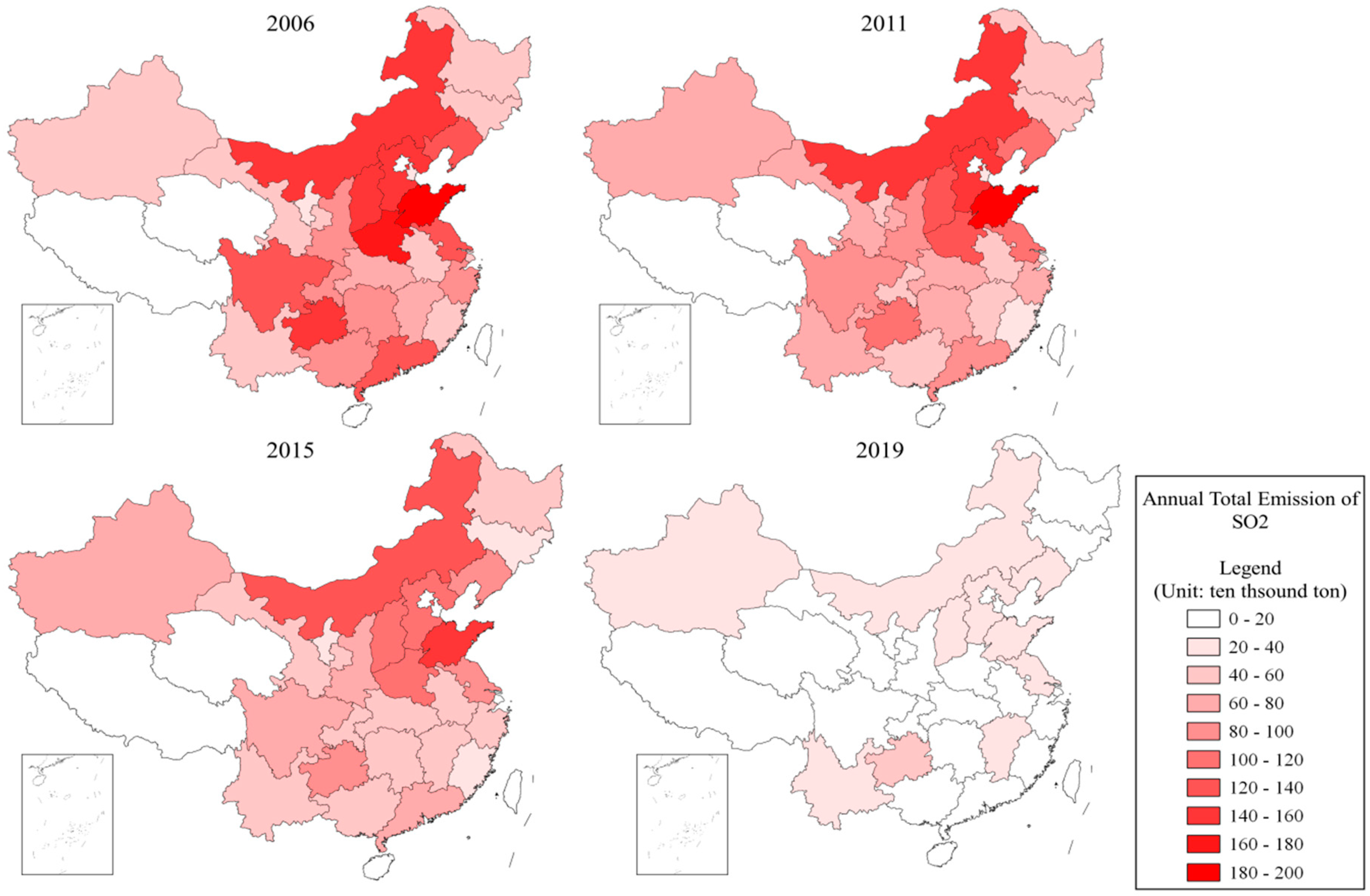
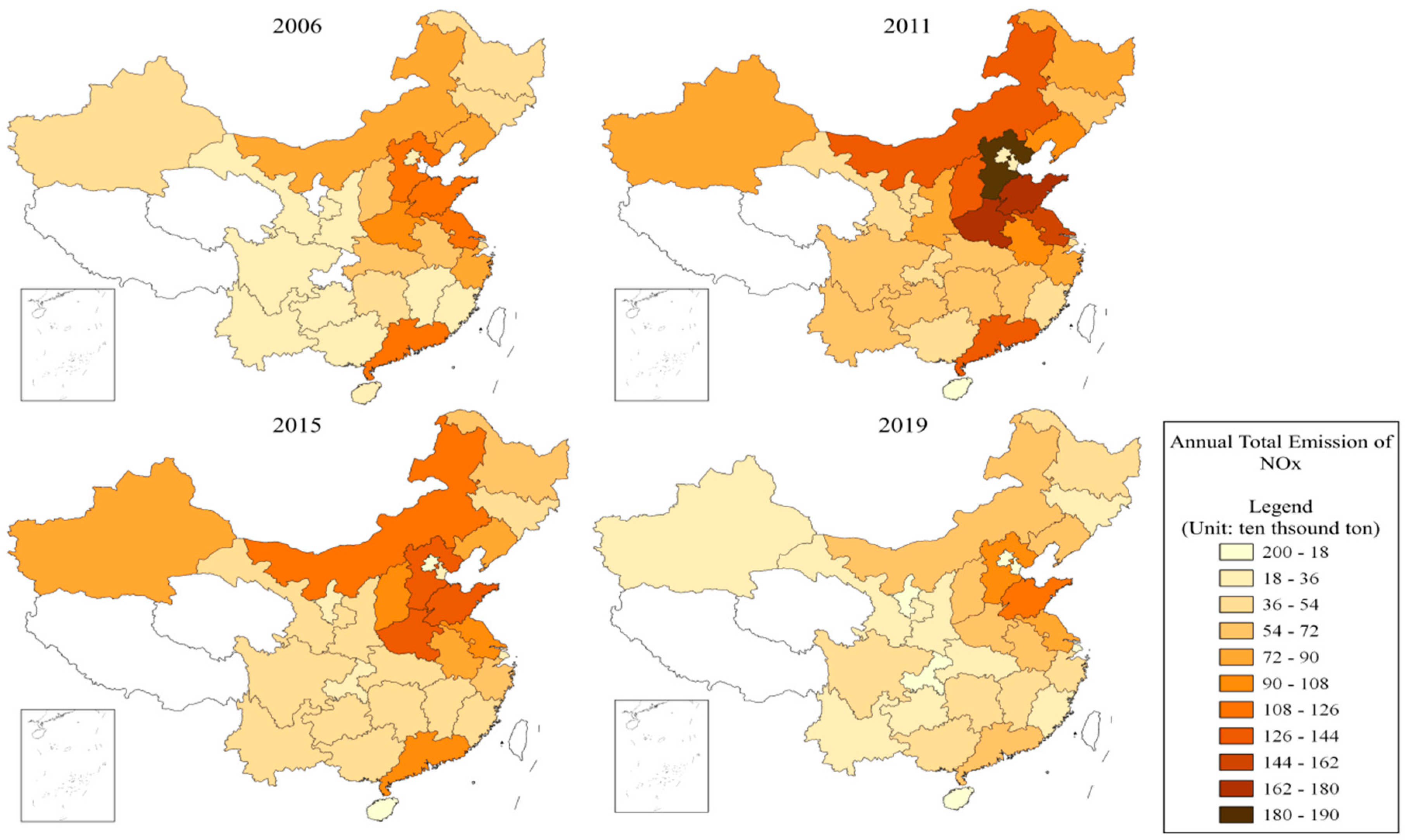
QGIS is an open source mapping software based on the geographic information system (GIS) [50,51], which can load the data into a geographical map and perform the spatial analysis [52,53,54], including the environment indices’ measuring and calculating [55]. In this study, we use QGIS to visualize and analyze hazardous air pollutants in 29 provinces of China. Figure 5, Figure 6 and Figure 7 show the total emission distribution of PM2.5, SO2, and NOx in China from 2006 to 2019. The heavier the color, the higher the discharge amount. It can be seen that air pollution is severe across China, especially in the North China Plain. China’s emissions of the three major air pollutants have not been decreasing all the time, but have shown a trend of first increasing first, then decreasing, and this trend has been more significant since 2015.

2.2.2. Explanatory Variables

The location entropy index is a measurement method that was introduced early to research on industrial agglomeration. It was first proposed by Huggett and then applied to subsequent research on agglomeration. The location entropy index measures the industrial agglomeration of a region, by using its number of employees or total output value. It has a high data availability and is suitable for basic research. Specifically, the locational entropy index [56] typically measures the ratio between the local and national percentage of employment, attributable to a particular industrial sector. Therefore, it is a “ratio between proportions”. Details are given below.
(1) Agglomeration index of manufacturing
M a g g i t = L j i t / L j t L i t / L t
M a g g i t is the agglomeration index of manufacturing, L j i t is the number of employees in industry j of region i in year t, L j t is the number of employees in industry j in year t, L i t is the number of employees of region i in year t, and L t is the total number of employees in the country in year t.
(2) Agglomeration index of producer services
S a g g i t = L j i t / L j t L i t / L t
S a g g i t is the agglomeration index of producer services, and the meanings of all other variables are the same as in Equation (4).
(3) Co-agglomeration index
C a g g i t = 1 | M a g g i t S a g g i t | M a g g i t + S a g g i t
C a g g i t is the co-agglomeration index, M a g g i t is the agglomeration index of manufacturing, and S a g g i t is the agglomeration index of producer services.
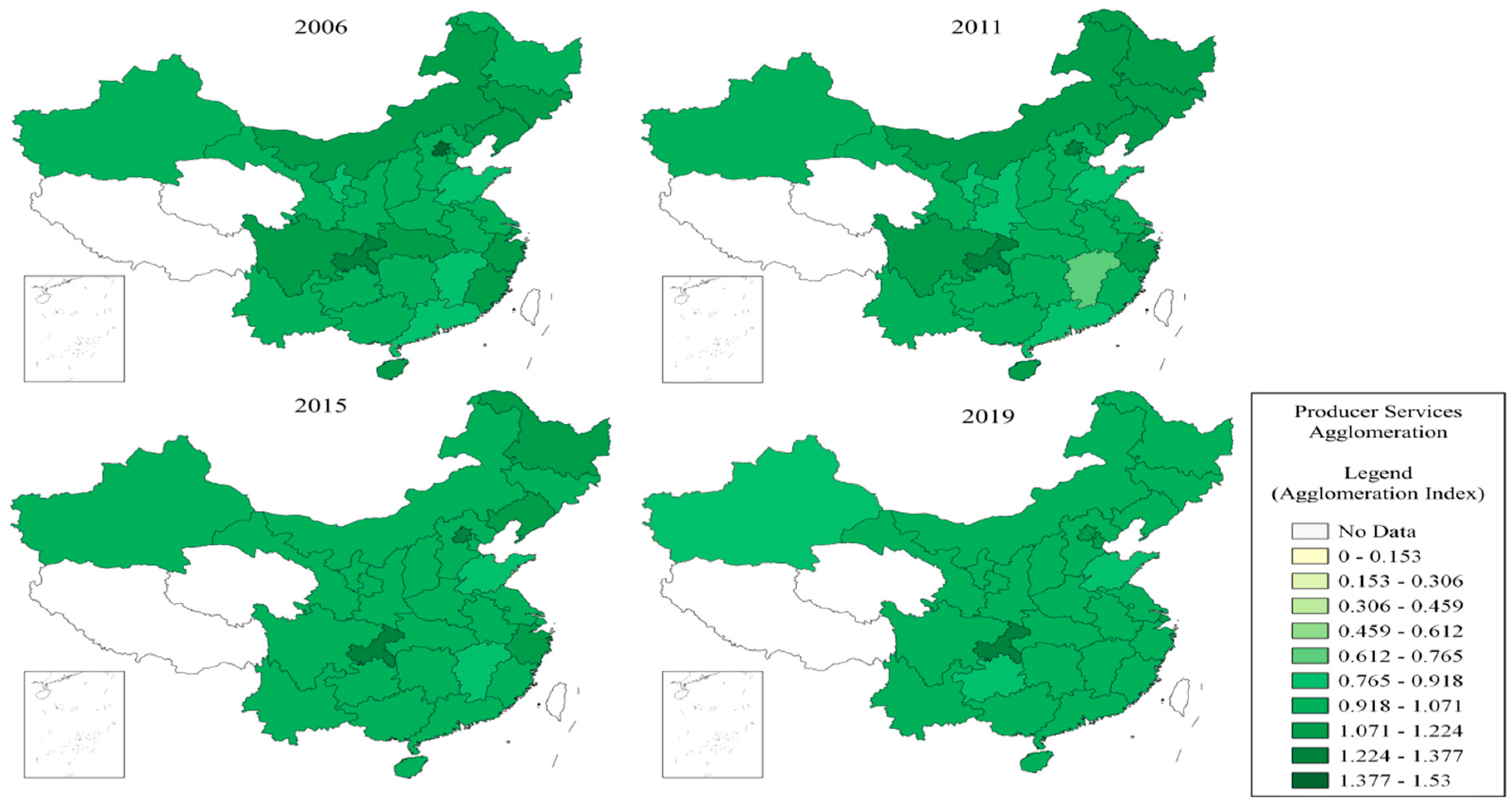
QGIS software was used to visualize and analyze the different industrial agglomerations in 29 provinces of China. Figure 8, Figure 9 and Figure 10 show the distribution of manufacturing agglomeration, producer services agglomeration n, and collaborative agglomeration in China from 2006 to 2019. The darker the color, the higher the degree of industrial agglomeration. It can be seen that the level of manufacturing agglomeration is higher in the central and western regions, and the distribution of producer services agglomeration is relatively balanced. The collaborative agglomeration of manufacturing and producer services is the highest in the eastern coastal regions.

2.3. Mediating Variables and Control Variables

2.3.1. Mediating Variables

(1) Energy consumption structure (Energy): The energy consumption structure is measured via the proportion of the coal consumption of the region of its total energy consumption. The industrial waste gases generated by the combustion of large amounts of coal constitute a major source of air pollution; therefore, studying the coal consumption of a region is of vital significance for measuring the air pollution of the region. Therefore, the energy consumption structure is taken as a mediating variable and its mediating role between the agglomeration of different industries and air pollution is explored.
(2) Human capital (RDhuman): The proportion of investment in human capital is measured using the proportion of R&D personnel in a region of its total number of employees. The fact that the Chinese government advocates sustainable development means that enterprises in China must transform traditional energy-intensive production modes into energy-conserving and environment-friendly production modes. This necessitates that there must be sufficient R&D personnel to engage in scientific and technological innovation. Thus, the number of R&D personnel in a region affects its overall R&D level, which further influences its production modes and consequently its air quality. Therefore, human capital is taken as a mediating variable and its mediating role between the agglomeration of different industries and air pollution is explored.

2.3.2. Control Variables

The control variables for this paper are Environmental regulation (ER), R&D investment intensity (RDintensity), Industrial structure (INS), Per capita GDP (pergdp), Square of per capita GDP (pergdp2), FDI (fcp), Regional openness (open), Urbanization level (city), and the control variable data sources are the China Environmental Statistics Yearbook & China Statistical Yearbook, China Statistical Yearbook of Science and Technology, China Statistical Yearbook of Science and Technology, CSMAR, China Statistical Yearbook, and NOAA/NGDC.
(1) Environmental regulation (ER) is expressed as the proportion of pollution governance investment in GDP divided by industrial characteristics. This expression reduces the effect of interregional differences in industrial structure. Strict environmental regulation can, to a certain extent, reduce the emissions of air pollutants. The specific measurement method is as follows:
E R i t = i n v e s t i t v a l u e i t / v a l u e i t G D P i t
where invest, value, and GDP denote the completion rate of industrial pollution governance investment, industrial added value, and nominal GDP, respectively.
(2) R&D investment intensity (RDintensity) is expressed as the proportion of regional R&D investment in regional GDP. A higher R&D investment helps enterprises strengthen their R&D innovation, raise productivity levels, and transform production modes, all of which can contribute to the improvement of regional air quality.
(3) Industrial structure (INS) is expressed as the proportion of the total output value of secondary industries of that of tertiary industries. The industrial structure measures the rationality of the overall industrial layout of a region.
(4) Per capita GDP (pergdp) is expressed as the ratio between regional GDP and regional total population. The effect of inflation has been eliminated using CPI.
(5) Square of per capita GDP (pergdp2) is expressed as the quadratic term of the actual per capita GDP and is used to validate whether there is an “Environmental Kuznets Curve”.
(6) FDI (fcp) expresses the proportion of regional FDI inventory in regional GDP in the current year and is used to explore the overall effect of total FDI on local environments. FDI inventory is calculated according to the perpetual inventory method as follows:
f c p i t = f c p i ( t 1 ) α f c p i ( t 1 ) + f d i i ( t )
f c p i ( 2006 ) = f d i i ( 2005 ) / ( g i + α )
where fcp denotes FDI inventory, fdi denotes FDI flow, α denotes the depreciation rate, set as 6%, and g i denotes the growth rate of per capita GDP.
(7) Regional openness (open) is expressed as the proportion of the regional total export-import volume of regional GDP. A region with higher openness may be able to attract more enterprises, which thus affects local air quality.
(8) Urbanization level (city) is expressed as the proportion of the urban population of a region of the total population of the region. A region with a higher urbanization level usually has relatively sound manufacturing and producer services, which exert more significant effects on air pollution.

2.4. Data Sources

2.4.1. Data Sources

The provincial panel data from 29 Chinese provinces (excluding Tibet, Qinghai, Hongkong, Macau, and Taiwan) from 2006 to 2019 are used in this study. To be specific, manufacturing covers 30 two-digit categories, and producer services cover 14 two-digit categories. Data on SO2, PM2.5, and NOx are derived from the China Statistical Yearbook on Environment. Other variables are provided in Table 1.

2.4.2. Descriptive Statistics of All Variables

Table 2 provides the descriptive statistics of all variables. Overall, the data are rational and do not contain any apparent outliers.

3. Empirical Test

Provincial panel data of China from 2006 to 2019 are used to perform the empirical test. “Panel fixed effects + clustering standard error”, the ordinary least squares (OLS), and the full generalized least squares (FGLS) method are adopted for econometric regression to assure the robustness of regression results. To a certain extent, this approach can reduce the statistical bias caused by heteroscedasticity. Considering the robustness of regression results, the FGLS panel econometrics model is employed as the basic regression model for analysis and testing, as this can better reduce heteroscedasticity and intra-group autocorrelation.

3.1. Baseline Regression

The baseline regression results of this paper are provided in the following, based on the setup of the above econometrics model. Table 3, Table 4 and Table 5 provide the baseline regressions of the effects of the agglomeration of manufacturing, the agglomeration of producer services, and co-agglomeration on three major air pollution sources, respectively. Baseline regressions are tested via “panel fixed effects + clustering standard error” and FGLS to guarantee the robustness of regression results, as shown below.
As shown in Table 3, Table 4 and Table 5, the agglomeration of manufacturing, the agglomeration of producer services, and their co-agglomeration have the most significant regression coefficient for PM2.5 (one of the three major air pollution sources). Specifically, the agglomeration of manufacturing increases the emissions of PM2.5 and SO2 into the air, while the agglomeration of producer services decreases the emission of PM2.5 and increases the emission of NOx into the air. Co-agglomeration of manufacturing and producer services can significantly reduce the emission of PM2.5, without exerting any significant effect on NOx or SO2. In terms of control variables, the coefficients of per capita GDP and the quadratic term of per capita GDP in Table 3, Table 4 and Table 5 are the opposite (Our regression test of the correlation coefficient between per capita GDP and quadratic term of per capita GDP in Table 3, Table 4 and Table 5, shows a high correlation between per capita GDP and quadratic term of per capita GDP correlated. The VIF test results (mean VIF=287.69) indicate the existence of multicollinearity in Equation (3). By comparing the regression results with and without the quadratic term of per capita GDP (Details in Table A1), it was found that the direction of the coefficients did not change. It is therefore inferred that the multicollinearity of the variables per capita GDP and quadratic term of per capita GDP does not affect the robustness of the regression results. Therefore, the relevant equations and regression results in the manuscript are plausible.). This validates the presence of the “Environmental Kuznets Curve”. That is, because of economic growth in a region, the environmental quality of the region first presents a deteriorating trend, then an improving trend afterward. Moreover, the coefficients of the control variable fcp are all significantly negative, suggesting that the FDI of a region can effectively reduce the emissions of PM2.5 and SO2 into the air.

3.2. Heterogeneity Test

3.2.1. Regional Heterogeneity

Based on interregional differences in economic development level and geographical environment across China, in this paper samples are classified into two categories (eastern China and central and western China) for regression and to explore how the effect of industrial agglomeration on air pollution varies across different regions. As shown in Table 6, the agglomeration of manufacturing increases both the emission of PM2.5 in central and western China and the emission of SO2 in eastern China. The agglomeration of producer services decreases both the emission of PM2.5 in central and western China and the emission of SO2 in eastern China and increases the emission of NOx in central and western China. Co-agglomeration decreases the emission of PM2.5 in central and western China.

3.2.2. Heterogeneity of Agglomeration

Glaeser et al. (1962) [57] proposed a classification of industrial agglomeration into diversified agglomeration and specialized agglomeration, reflecting the economic effects of the industrial agglomeration of different industries and that of the same industry on the economy, respectively. More specifically, diversified agglomeration (Rdi) and specialized agglomeration (Com) are constructed in reference to the method proposed by Martin et al. (2011) [20,25,58], as detailed below:
R d i i t = l n ( ( 1 / ( j j | L j i t L i t L j t L t | ) ) + 1 )
C o m i t = l n ( ( 1 / H e r f j i t ) + 1 )
where R d i i t measures the Jacob externalities of province i in year t, i.e., the economic diversity the industry faces, C o m i t denotes the specialized agglomeration degree of province i in year t, and H e r f j c t = j ϵ i t ( L j i t L i t ) 2 denotes the Herfindahl index, which can better reflect the monopoly degree of the industry.
As shown in Table 7, the diversified agglomeration of manufacturing increases both the emissions of the three major air pollutants in eastern China and the emission of PM2.5 in central and western China, and decreases the emission of SO2 in central and western China. The specialized agglomeration of manufacturing decreases both the emissions of the three major air pollutants in eastern China and the emission of PM2.5 in central and western China. The diversified agglomeration of producer services increases the emission of PM2.5 in eastern China. The specialized agglomeration of producer services decreases the emissions of all three of the major air pollutants in eastern China.

3.3. Robustness Test

To guarantee the robustness of the baseline regression results, in this paper the relationship between agglomeration and three major air pollution sources is further validated. First, when we clean the underlying data, we mainly use methods such as logarithmic and uniform measures of the main variables to reduce the heteroskedasticity in the regressions, so the effect of bias from outliers can be greatly reduced. Second, Lag term, spatial correlation test, and instrumental variables are used to test the baseline regression [59,60,61,62,63].

3.3.1. First-Phase Lag

The number of enterprises in the initial stage of agglomeration was small, making it probable that the impact of air pollution had not manifested yet. With the continuous increase in the number of enterprises in an agglomeration area, the energy consumption of that agglomeration area increased, which had a certain impact on regional air pollution. The emissions of air pollutants in the current stage might be affected by previous air pollution. On that account, in this paper, the method of first-phase lag of core explanatory variables is adopted to validate the results of baseline regression [59]. As shown in Table 8, the effects of the agglomeration of manufacturing, the agglomeration of producer services, and co-agglomeration on PM2.5, SO2, and NOx after first-phase lag are consistent with the baseline regression results. That is, all three agglomeration patterns significantly affect PM2.5 emissions into the air but exert no significant effect on either of the other two air pollutants (SO2, and NOx). This validates the correctness of baseline regression.

3.3.2. Spatial Correlation

(1)
Spatial correlation test
Air pollution has a spatial correlation in most cases, and therefore ignoring spatial correlation may lead to biased results. For this reason, in this paper, Moran’s index is used to perform the correlation test first. Moran’s index [60] reflects the degree of similarity between the attribute values of spatially contiguous or spatially adjacent regional units, and is calculated via Equation (12):
M o r a n I = [ i = 1 n j = 1 n w i j ( x i x ¯ ) ( x j x ¯ ) ] / [ i = 1 n ( x i x ¯ ) 2 ]
Table 9 provides the Moran’s index values of PM2.5, NOx, and SO2 emissions for 29 provinces from 2006 to 2019. Only the coefficients of PM2.5 are significant, the emission of PM2.5 into the air shows spatial correlation, but neither NOx nor SO2 presents any clear spatial correlation. This further testifies to the robustness of regression in the baseline model. Therefore, this paper only considers the spatial correlation of PM2.5, and further tests the robustness of the regression results.
(2)
Regression results of spatial econometrics model
To further validate the availability of the baseline model’s settings, the Spatial Durbin Model (SDM) [61,62] is adopted for regression based on the spatial correlation test. Table 10 indicates that the agglomeration of manufacturing increases the emission of PM2.5 into the air, while the agglomeration of producer services and co-agglomeration effectively reduces the emissions of PM2.5 into the air, which is consistent with the directions of the regression coefficients of PM2.5 in Table 3, Table 4 and Table 5. This consistency suggests that the setup of the baseline model in this paper is reliable.

3.3.3. Instrumental Variables

The two-stage least squares (2SLS) method is adopted to identify suitable instrumental variables and further address the potential endogenous problem with industrial agglomeration. Historical population data are used to construct instrumental variables. Because of the externalities of instrumental variables, relatively fixed variables such as population, geography, and history can serve as ideal instrumental variables. Thus, in reference to the practice of Combes et al. (2010) [63], in this paper, historical population data are employed as instrumental variables of industrial agglomeration. To be specific, the logarithms of the numbers of employees engaged in manufacturing and producer services at the provincial level in 2000 are selected as instrumental variables of industrial agglomeration. Econometric regression is performed by 2SLS. As shown in Table 11, after the endogenous problem is solved, the regression results of the instrumental variable are basically consistent with baseline regression. In summary, the instrumental variable selected in this paper is rational. According to the results of econometric regression, the effects of the agglomeration of manufacturing, the agglomeration of producer services, and co-agglomeration on three major air pollution sources are consistent with data shown in Table 3, even when the potential endogenous problem is considered. That is, the agglomeration of manufacturing increases the emissions of PM2.5 into the air, while that of producer services and the co-agglomeration of manufacturing and producer services decreases it. In addition, the regression coefficients are all higher than the baseline regression model, indicating that in the baseline regression, the effect of agglomeration on air pollution may be underestimated. However, the core conclusion of this paper is still valid.

3.4. Mechanism Test

As shown in the above analysis, the energy consumption structure and human capital of a region affect the air pollutant emissions of the region. Therefore, energy consumption structure and human capital are used as mediating variables to set up the econometrics model and verify whether they have mediating roles [59,64,65,66,67].

3.4.1. Energy Consumption Structure

The following system of equations is created to identify the mediating role of energy consumption structure:
l n E n e r g y i t = β 0 + β 1 l n a g g i t + β 2 X i t + λ i t + ε i t
l n P o l l u t i o n i t = a 0 + a 1 l n a g g i t + a 2 X i t + a 3 l n E n e r g y i t + λ i t + ε i t
where t and i denote year and province, respectively, Energy denotes the energy consumption structure, which can satisfactorily reflect the situations of energy consumption by various industries, α 0 , β 0 , and a 0 are constant terms, α 1 , β 1 , a 1 , and a 3 are parameters to be estimated, X i t is the set of control variables, λ i t represents time and individual fixed effects, and ε i t is a stochastic disturbance term. The continuous variables in these models are taken from the common logarithm, which can unify the dimensionless parameters, and reduce the heteroscedasticity by minimizing the influence of the outliers [50].
Table 12, Table 13 and Table 14 provide the regression results of Equations (13) and (14). The effect of the agglomeration of manufacturing on energy consumption structure in Equation (13) is significantly positive. In Equation (14), the energy consumption structure has a significantly positive effect on PM2.5, but it has no significant effect on either SO2 or NOx. The results suggest that the energy consumption structure is a mediating variable between the agglomeration of manufacturing and PM2.5, i.e., the agglomeration of manufacturing increases PM2.5 emission via the energy consumption structure. In the agglomeration of producer services, the effect of the agglomeration of producer services on energy consumption structure in Equation (13) is non-significant. In Equation (14), the energy consumption structure has a significant positive effect on PM2.5, but the agglomeration of producer services has no significant effect on PM2.5, SO2, or NOx. These results indicate that the energy consumption structure is not a mediating variable between the agglomeration of producer services and air pollutants. This is because the production modes of producer services are generally green and barely involve coal consumption. Consequently, the energy consumption structure exerts no significant effect on producer services. In the case of co-agglomeration, the effect of co-agglomeration on energy consumption structure in Equation (13) is significantly negative. In Equation (14), energy consumption structure has a significantly positive effect on PM2.5, while co-agglomeration has no significant effect on PM2.5, SO2, or NOx. The results clearly show that the energy consumption structure is not a mediating variable between co-agglomeration and air pollutants. One possible explanation is that the policies introduced by the state to promote energy conservation and emission reduction and to encourage the development of the service industry have not yet fully exerted their effects. While co-agglomeration indeed changes the energy consumption structure, it takes time for co-agglomeration to manifest its full effect on air pollution.

3.4.2. Human Capital

According to the above elaboration on mechanisms, the human capital of a region may mitigate the air pollution of that region. To test whether human capital plays a mediating role between industrial agglomeration and air pollution, this paper has designed the following mediating effect model [59,64,65,66,67]:
l n R D h u m a n i t = β 0 + β 1 l n a g g i t + β 2 X i t + λ i t + ε i t
l n P o l l u t i o n i t = a 0 + a 1 l n a g g i t + a 2 X i t + a 3 l n R D h u m a n i t + λ i t + ε i t
where t and i denote year and province, respectively, and R D h u m a n denotes human capital, which reflects the importance of R&D personnel in environmental governance. X i t is the set of control variables, λ i t represents time and individual fixed effects, and ε i t is a stochastic disturbance term. The continuous variables in this model are taken by the common logarithm, which can unify the dimensionless parameters, and reduce the heteroscedasticity by minimizing the influence of the outliers [49].
Table 15, Table 16 and Table 17 provide the regression results of Equation (15) and Equation (16). In terms of the agglomeration of manufacturing, the effect of the agglomeration of manufacturing on human capital in Equation (15) is negative. In Equation (16), human capital exerts a significantly negative effect on PM2.5 but has no significant effect on either SO2 or NOx. This suggests that human capital is not a mediating variable between the agglomeration of manufacturing and PM2.5. The effect of the agglomeration of producer services on human capital in Equation (15) is significantly positive, possibly because the green production modes of producer services raise the requirements for R&D and promote the improvement of human capital. In Equation (16), human capital has a significantly negative effect on PM2.5, suggesting that human capital is a mediating variable between the agglomeration of producer services and PM2.5. That is, agglomeration of producer services can improve human capital and further decrease the emission of PM2.5 into the air. In the case of co-agglomeration, the effect of co-agglomeration on human capital in Equation (15) is non-significant. In Equation (16), human capital has a significant negative effect on PM2.5 but has no significant effect on either SO2 or NOx. This suggests that human capital is not a mediating variable between co-agglomeration and air pollutants. One possible reason is that R&D personnel are typical professional technicians who have low mobility between industries. Therefore, human capital does not play a mediating role.

4. Result Discussion

4.1. Different Industrial Agglomeration Patterns

As implied by the baseline regression results of this paper in Table 3, Table 4 and Table 5, agglomeration of manufacturing increases the emissions of PM2.5 into the air, while the agglomeration of producer services and the co-agglomeration of manufacturing and producer services decreases it. Further, manufacturing enterprises are industrial enterprises that mostly consume coal, petroleum, and other raw materials in the production process, and their energy-intensive production modes often adversely impact regional air quality. By contrast, enterprises engaging in producer services (tertiary industries) largely serve manufacturing enterprises and consume less pollution-intensive energies in the production process. Their green production modes decrease air pollution locally. The co-agglomeration of these two industries realizes the interindustry sharing of spillover effects, rationalizes regional industrial structure, and reduces the emissions of air pollutants.

4.2. Heterogeneity

Regarding regional division in China, all three agglomeration patterns have significant effects on PM2.5 emissions in central and western China, as shown in Table 6 and Table 7. As expected, they also affect PM2.5 emissions in eastern China, but not significantly. This is possible because China’s natural energy resources are mostly concentrated in its central and western provinces. For instance, Shanxi and Henan have abundant coal resources, for which numerous manufacturing enterprises have accumulated in these provinces, which further increases the PM2.5 emissions [68,69]. In contrast, producer services consume little energy-intensive resources and can effectively inhibit the emission of PM2.5 into the air. The same is true for the co-agglomeration of industries. SO2 differs from PM2.5 in this regard. That is, the emission of SO2 in eastern China is increased by the agglomeration of manufacturing but significantly decreased by the agglomeration of producer services. Judging from the industrial heterogeneity of agglomeration, diversified agglomeration increases the emission of PM2.5 in eastern China and central and western China and the emissions of NOx and SO2 in eastern China in the case of manufacturing. It also increases the emission of PM2.5 in eastern China in the case of producer services. By contrast, specialized agglomeration decreases the emission of PM2.5 in eastern China and central and western China and the emissions of NOx and SO2 in eastern China in the case of manufacturing. It also decreases the emissions of PM2.5, NOx, and SO2 in eastern China in the case of producer services. Clearly, specialized agglomeration of the same industry plays a stronger role in governing interregional air pollution. A possible explanation is that, by virtue of the massively specialized agglomeration of homogeneous enterprises within the same industry, these enterprises can share pollution discharge facilities and advanced production technologies in the agglomeration area, transform their production modes, and engage in sustainable green production.

4.3. Mediating Mechanism Test

Therefore, energy consumption structure and human capital are used as mediating variables to explore the mediating mechanisms between industrial agglomeration and air pollution. The above analysis in Table 12, Table 13, Table 14, Table 15, Table 16 and Table 17 shows that manufacturing enterprises constitute a major contributor to regional energy consumption, while enterprises engaged in producer services consume little energy in practical production. As a result, manufacturing enterprises increase PM2.5 emissions through energy consumption. Industrial agglomeration also improves local environmental quality through R&D investment. Currently, driven by increasingly strict environmental policies implemented throughout China, enterprises attach greater importance to their sustainable development. In practical production, enterprises intensify their R&D investment to increase production efficiency and adopt clean energies for production to reduce air pollutant emissions. Human capital plays a mediating role and can decrease PM2.5 emissions in the agglomeration of producer services.

5. Conclusions and Suggestions

5.1. Research Summary

Provincial panel data of China from 2006 to 2019 are used in this paper. The generalized FGLS panel econometric model is combined with SDM and the relationships between industrial agglomeration and three major air pollution sources are systematically studied. The transmission mechanisms underlying the effects of different industrial agglomeration patterns on these air pollution sources are further explored. The results show that, among these air pollution sources, only PM2.5 presents a significant spatial correlation. That is, only the emission of PM2.5 is significantly affected by the agglomeration of manufacturing, the agglomeration of producer services, and co-agglomeration. More specifically, the agglomeration of manufacturing increases the emission of PM2.5, while that of producer services and co-agglomeration effectively reduce the emission of PM2.5 into the air. Furthermore, in terms of regional division in China, agglomeration of manufacturing increases the emissions of harmful air pollutants in central and western China, while agglomeration of producer services decreases them. Specialized agglomeration is more conducive to the governance of air pollution. Finally, the research on mechanisms shows that the agglomeration of manufacturing deteriorates the energy consumption structure and increases the emissions of harmful air pollutants into the air, while the agglomeration of producer services, benefiting from human capital, decreases the emission of PM2.5 into the air and improves air quality.
Why does industrial agglomeration have a significant effect on PM2.5 but not on NOx and SO2? A possible explanation for this is that PM2.5 has a wider range of sources than NOx and SO2 and is more damaging to the environment. The main sources of PM2.5 are not only industrial emissions, but also emissions from vehicle exhaust, pollution from burning coal for residential use, and the felling of trees by residents to expand their living areas, all of which degrade the natural environment. The industrial agglomeration will lead to more employment opportunities, which will attract more employees to gather near the industrial area to produce and live, traffic congestion and residential life will increase the production of vehicle exhaust and domestic exhaust, and thus PM2.5 significantly aggravate air pollution. According to Section 3.3.2, the spatiality of the three major air pollutants was also detected and only PM2.5 had a significant spatial correlation, while NOx and SO2 had no significant spatial correlation, further supporting the original conclusion. The above conclusions show China’s success in NOx and SO2 air management, and as in the basic conclusions in Figure 2 and Figure 3, NOx and SO2 emissions are basically on par with developed countries such as the UK and the US. However, although PM2.5 emissions are on a downward trend, it is still at a high-level overall (Figure 1), which requires us to continue to promote the agglomeration of productive services, further optimize the industrial structure, and use renewable energy and reduce PM2.5 emissions.

5.2. Policy Suggestions and Future Research

In summary, some suggestions on containing and reducing the environmental pollution during the processing of industrial upgrading are given as follows: first, the top priority is the optimization of the industrial structure, a rational industrial structure means that, to improve economic efficiency, it is required to adjust the initially unreasonable industrial structure at a certain stage of economic development according to the level of science and technology, the structure of consumer demand, the basic quality of the population and the conditions of resources [70,71,72], to achieve a rational allocation of production factors and the coordinated development of various industries, as a rational industrial structure plays a vital part in improving regional environmental quality. Second, it is necessary to intensify corporate R&D investment, cultivate R&D personnel, and raise the human capital level, as these factors constitute the foundation for increasing production efficiency and transforming production modes, as well as the source of sustainable economic development. Thirdly, the role of education in the overall environmental protection cannot be ignored, and the government can enhance environmental protection by increasing the publicity of environmental protection, integrating environmental education into teaching and practice, giving appropriate policy concessions to environmental protection enterprises, and raising residents’ awareness of environmental protection. Finally, efforts should be directed to further optimize the industrial structures of different regions and promote the balanced development of manufacturing and producer services among regions, to thus alleviate the imbalance in environmental quality between eastern China and central and western regions, reduce the limitations of the regional effect of initial resources, and promote economic development towards a greener and more environmentally friendly direction. In the future, higher utilization of renewable energies such as photovoltaic, wind power, and biomass, are strongly needed to substitute for conventional power, as the Chinese government is committed to building a clean, low-carbon, safe and efficient energy system, and renewable energy sources can effectively improve air quality.
Some deficiencies exist in this paper. Firstly, due to the data availability, some potential sources such as carbon monoxide (CO), volatile organic compounds (VOC), or smoke dust may also have a relationship with industrial agglomeration, which has not been probed in this study; secondly, these air pollutants may also have linkages with SO2, PM2.5, and NOx, which have been proved in previous studies [73,74] but neglected here; lastly, more methods are still needed to ensure the robustness of our results. Therefore, to enhance higher reliability and comprehensiveness, it is essential to incorporate possible interactive atmospheric pollutants in future studies, and a series of causal inference studies should be carried out.

Author Contributions

Conceptualization, J.L. and P.Y.; methodology, J.L. and W.M.; software, P.Y., J.L. and W.M.; validation, J.L. and W.M.; formal analysis, J.L. and W.M.; investigation, J.L.; data curation, P.Y., J.L. and W.M.; writing—original draft preparation, J.L.; writing—review and editing, J.L., P.Y. and W.M.; visualization, P.Y.; supervision, H.Z.; project administration, H.Z. All authors have read and agreed to the published version of the manuscript.

Funding

This research was funded by the “Fundamental Research Funds for the Central Universities” from Zhongnan University of Economics and Law (grant No.202111015) and the Research Start-up Fund (Grant No.kyqd(sk)2022012) from Hainan University.

Institutional Review Board Statement

Not applicable.

Informed Consent Statement

Not applicable.

Data Availability Statement

All data generated or analyzed during this study are included in this published article.

Conflicts of Interest

The authors declare no conflict of interest. They also declare no financial or personal relationships with other people or organizations that could inappropriately bias the results presented in this manuscript.

Abbreviation

FGLSFull Generalized Least Squares
OLSOrdinary Least Square
GDPGross Domestic Product
R&DResearch and Development
QGISQuantum Geographic Information System
CPIConsumer Price Index
FDIForeign Direct Investment
SDMSpatial Dubin Model
2SLSTwo-stage Least Squares

Appendix A

Table A1. Baseline regression results for GDP per capita only.
OLS+FEFGLSOLS+FEFGLSOLS+FEFGLS
PM2.5PM2.5NOxNOxSO2SO2
Magg6.663 *4.780 **4.7611.49532.6208.611 *
(3.408)(1.982)(9.551)(4.061)(19.587)(4.699)
ER−3.108−1.688−16.7469.114−2.9791.016
(13.368)(7.409)(52.828)(15.500)(61.016)(22.041)
RDintensity−1.680−2.214 **−1.199−1.871−7.770−5.418 **
(1.422)(1.024)(3.128)(2.065)(6.209)(2.580)
INS−1.4660.9704.727−1.9559.6813.427
(2.891)(1.435)(9.578)(3.661)(10.313)(3.889)
lnpergdp1.8141.14128.268 *15.128 ***44.008 *10.663 *
(4.265)(2.261)(15.566)(5.739)(21.700)(6.238)
fcp−7.665−4.139−15.416−7.926−70.776−52.014 ***
(7.282)(5.268)(24.486)(14.984)(54.588)(19.809)
open0.623−1.12229.499 **16.009**2.0315.308
(4.800)(2.641)(13.831)(7.067)(21.618)(7.636)
city−0.048−0.160−0.7110.109−3.958***−1.832 ***
(0.360)(0.149)(0.610)(0.344)(0.800)(0.406)
_cons29.01452.681**−205.799−153.684 ***−174.196109.924 *
(32.894)(20.885)(132.732)(53.896)(193.941)(60.640)
N406406406406406406.000
R20.699 0.626 0.781
timeYesYesYesYesYesYes
ind Yes Yes Yes
Note: ① ***, **, * denote significance levels of 1%, 5%, and 10%, respectively; values in square brackets below the coefficients are robust standard errors. ② “time” represents time-fixed effects. ③ “ind” represents individual fixed effects.

References

  1. Qian, L.; Song, J.; Hao, H.; Wang, Y. Economic growth and pollutant emissions in China: A spatial econometric analysis. Stoch. Environ. Res. Risk Assess. 2014, 28, 429–442. [Google Scholar]
  2. He, C.; Huang, Z.; Ye, X. Spatial heterogeneity of economic development and industrial pollution in urban China. Stoch. Environ. Res. Risk Assess. 2014, 28, 767–781. [Google Scholar] [CrossRef]
  3. Zheng, X.; Yu, Y.; Wang, J.; Deng, H. Identifying the determinants and spatial nexus of provincial carbon intensity in china: A dynamic spatial panel approach. Reg. Environ. Change 2014, 14, 1651–1661. [Google Scholar] [CrossRef] [Green Version]
  4. Li, X.; Xu, Y.; Yao, X. Effects of industrial agglomeration on haze pollution: A Chinese city-level study. Energy Policy 2021, 148, 111928. [Google Scholar] [CrossRef]
  5. Cao, C.; Lee, X.; Liu, S.; Schultz, N.; Xiao, W.; Zhang, M.; Zhao, L. Urban heat islands in China enhanced by haze pollution. Nat. Commun. 2016, 7, 12509. [Google Scholar] [CrossRef]
  6. Yu, H.C.; Liu, Y.; Liu, C.L. Spatiotemporal variation and inequality in China’s economic resilience across cities and urban agglomerations. Sustainability 2018, 10, 4754. [Google Scholar] [CrossRef] [Green Version]
  7. Wang, S.; Jia, M.; Zhou, Y.; Fan, F. Impacts of changing urban form on ecological efficiency in China: A comparison between urban agglomerations and administrative areas. J. Environ. Plan. Manag 2019, 63, 1834–1856. [Google Scholar] [CrossRef]
  8. Fan, F.; Lian, H.; Liu, X.; Wang, X. Can environmental regulation promote urban green innovation efficiency? An empirical study based on Chinese cities. J. Clean. Prod 2020, 287, 125060. [Google Scholar] [CrossRef]
  9. Sun, C.Z.; Yan, X.D.; Zhao, L.S. Coupling efficiency measurement and spatial correlation characteristic of water-energy-food nexus in China. Resour. Conserv. Recycl. 2021, 164, 105151. [Google Scholar] [CrossRef]
  10. Chen, C.C.; Sun, Y.; Lan, Q.; Jiang, F. Impacts of industrial agglomeration on pollution and ecological efficiency-A spatial econometric analysis based on a big panel dataset of China’s 259 cities. J. Clean. Prod. 2020, 258, 120721. [Google Scholar] [CrossRef]
  11. Lu, W.; Tam, V.W.; Du, L.; Chen, H. Impact of industrial agglomeration on haze pollution: New evidence from Bohai Sea Economic Region in China. J. Clean. Prod. 2021, 280, 124414. [Google Scholar] [CrossRef]
  12. Liu, S.; Zhu, Y.; Du, K. The impact of industrial agglomeration on industrial pollutant emission: Evidence from China under New Normal. Clean Technol. Environ. Policy 2017, 19, 2327–2334. [Google Scholar] [CrossRef]
  13. Su, Y.; Yu, Y.Q. Spatial agglomeration of new energy industries on the performance of regional pollution control through spatial econometric analysis. Sci. Total Environ. 2020, 704, 135261. [Google Scholar] [CrossRef] [PubMed]
  14. Virkanen, J. Effect of urbanization on metal deposition in the bay of Töölönlahti, Southern Finland. Mar. Pollut. Bull 1998, 36, 729–738. [Google Scholar] [CrossRef]
  15. Frank, A. Urban air quality in larger conurbations in the European Union. Environ. Modell. Softw 2001, 16, 399–414. [Google Scholar]
  16. Markusen, J.R.; Venables, A.J. Foreign direct investment as a catalyst for industrial development. Eur. Econ. Rev 1999, 43, 335–356. [Google Scholar] [CrossRef] [Green Version]
  17. Shen, N.; Peng, H. Can industrial agglomeration achieve the emission-reduction effect? Socio-Econ. Plan. Sci. 2020, 75, 100867. [Google Scholar] [CrossRef]
  18. Peng, H.; Wang, Y.; Hu, Y.; Shen, H. Agglomeration production, industry association and carbon emission performance: Based on spatial analysis. Sustainability 2020, 12, 7234. [Google Scholar] [CrossRef]
  19. Li, X.; Zhu, X.; Li, J.; Gu, C. Influence of different industrial agglomeration modes on Eco-efficiency in China. Int. J. Environ. Res. Public Health 2021, 18, 13139. [Google Scholar] [CrossRef]
  20. Shen, N.; Zhao, Y.; Wang, Q. Diversified agglomeration, specialized agglomeration, and emission reduction effect—A Nonlinear Test Based on Chinese City Data. Sustainability 2018, 10, 2002. [Google Scholar] [CrossRef] [Green Version]
  21. Paci, R.; Usai, S. Externalities, knowledge spillovers and the spatial distribution of innovation. ERSA Conf. Pap. Eur. Reg. Sci. Assoc. 2000, 49, 381–390. [Google Scholar]
  22. Abdel-Rahman, H.; Fujita, M. Product variety, marshallian externalities, and city sizes. J. Reg. Sci. 1990, 30, 165–183. [Google Scholar] [CrossRef]
  23. Ma, R.; Wang, C.; Jin, Y.; Zhou, X. Estimating the effects of economic agglomeration on haze pollution in yangtze river delta china using an econometric analysis. Sustainability 2019, 11, 1893. [Google Scholar] [CrossRef] [Green Version]
  24. Hu, Z.; Cai, Y. Industrial agglomeration and industrial SO2 emissions in China’s 285 cities: Evidence from multiple agglomeration types. J. Clean. Prod. 2022, 353, 131675. [Google Scholar]
  25. Pei, Y.; Zhu, Y.; Liu, S.; Xie, M. Industrial agglomeration and environmental pollution: Based on the specialized and diversified agglomeration in the Yangtze River Delta. Environ. Dev. Sustain. 2020, 23, 4061–4085. [Google Scholar] [CrossRef]
  26. Cheng, Z. The spatial correlation and interaction between manufacturing agglomeration and environmental pollution. Ecol. Indic. 2016, 61, 1024–1032. [Google Scholar] [CrossRef]
  27. Zhu, Y.; Xia, Y. Industrial agglomeration and environmental pollution: Evidence from China under New Urbanization. Energy Environ. 2018, 30, 1010–1026. [Google Scholar] [CrossRef]
  28. Wu, J.; Xu, H.; Tang, K. Industrial agglomeration, CO2 emissions and regional development programs: A decomposition analysis based on 286 Chinese cities. Energy 2021, 225, 120239. [Google Scholar] [CrossRef]
  29. Selden, T.M.; Song, D. Environmental quality and development: Is there a Kuznets Curve for air pollution emissions? J. Environ. Econ. Manag. 1994, 27, 147–162. [Google Scholar] [CrossRef]
  30. Liu, J.; Qu, J.; Zhao, K. Is China’s development conforms to the Environmental Kuznets Curve hypothesis and the pollution haven hypothesis? J. Clean. Prod. 2019, 234, 787–796. [Google Scholar] [CrossRef]
  31. Cansino, J.M.; Román-Collado, R.; Molina, J.C. Quality of institutions, technological progress, and pollution havens in Latin America. An analysis of the Environmental Kuznets Curve hypothesis. Sustainability 2019, 11, 3708. [Google Scholar] [CrossRef] [Green Version]
  32. Sarkodie, S.A.; Strezov, V. Effect of foreign direct investments, economic development and energy consumption on greenhouse gas emissions in developing countries. Sci. Total Environ. 2019, 646, 862–871. [Google Scholar] [CrossRef] [PubMed]
  33. Gill, A.R.; Viswanathan, K.K.; Hassan, S. The Environmental Kuznets Curve (EKC) and the environmental problem of the day. Renew. Sust. Energ. Rev. 2018, 81, 1636–1642. [Google Scholar] [CrossRef]
  34. List, J.A.; Catherine, Y.C. The effects of environmental regulations on foreign direct investment. J. Environ. Econ. Manag. 2000, 40, 1–20. [Google Scholar] [CrossRef] [Green Version]
  35. AI-Mulali, U.; Weng-Wai, C.; Sheau-Ting, L.; Mohammed, A.H. Investigating the environmental Kuznets curve (EKC) hypothesis by utilizing the ecological footprint as an indicator of environmental degradation. Ecol. Indic 2015, 48, 315–323. [Google Scholar] [CrossRef]
  36. Jie, H. Pollution haven hypothesis and environmental impacts offoreign direct investment: The case of industrial emission of sulfur dioxide (SO2) in Chinese provinces. Ecol. Econ 2006, 60, 228–245. [Google Scholar]
  37. Baomin, D.; Jiong, G.; Xin, Z. FDI and environmental regulation: Pollution haven or a race to the top? J. Regul. Econ 2012, 41, 216–237. [Google Scholar]
  38. Kheder, S.B.; Zugravu, N. Environmental regulation and French firms location abroad: An economic geography model in an international comparative study. Ecol. Econ 2012, 77, 48–61. [Google Scholar] [CrossRef]
  39. Baldwin, J.R.; Brown, W.M.; Rigby, D.L. Agglomeration economics: Microdata panel estimates from Canadian manufacturing. J. Reg. Sci 2010, 50, 915–934. [Google Scholar] [CrossRef]
  40. Drucker, J.; Feser, E. Regional industrial structure and agglomeration economies: An analysis of productivity in three manufacturing industries. Reg. Sci. Urban Econ 2012, 42, 1–14. [Google Scholar] [CrossRef]
  41. Ye, P.; Xia, S.; Xiong, Y.; Liu, C.; Li, F.; Liang, J.; Zhang, H. Did an ultra-low emissions policy on coal-fueled thermal power reduce the harmful emissions? Evidence from three typical air pollutants abatement in China. Int. J. Environ. Res. Public Health 2020, 17, 8555. [Google Scholar] [CrossRef] [PubMed]
  42. Zhou, X.; Feng, C. The impact of environmental regulation on fossil energy consumption in China: Direct and indirect effects. J. Clean. Prod. 2017, 142, 3174–3183. [Google Scholar] [CrossRef]
  43. Hao, Y.; Song, J.; Shen, Z. Does industrial agglomeration affect the regional environment? Evidence from Chinese cities. Environ. Sci. Pollut. Res. 2021, 29, 7811–7826. [Google Scholar] [CrossRef] [PubMed]
  44. Verhoef, E.T.; Nijkamp, P. Externalities in urban sustainability: Environmental versus localization-type agglomeration externalities in a general spatial equilibrium model of a single-sector monocentric industrial city. Ecol. Econ 2002, 40, 157–179. [Google Scholar] [CrossRef] [Green Version]
  45. Zhu, Y.; Du, W.; Zhang, J. Does industrial collaborative agglomeration improve environmental efficiency? Insights from China’s population structure. Environ. Sci. Pollut. Res. 2021, 29, 5072–5091. [Google Scholar] [CrossRef]
  46. Thiel, C.; Nijs, W.; Simoes, S.; Schmidt, J.; Zyl, A.V.; Schmid, E. The impact of the EU car CO2 regulation on the energy system and the role of electro-mobility to achieve transport decarbonisation. Energy Policy 2016, 96, 153–166. [Google Scholar] [CrossRef]
  47. Ehrlich, P.R.; Holdren, J.R. Impact of population growth. Science 1971, 171, 1212–1217. [Google Scholar] [CrossRef]
  48. Dietz, T.; Rosa, E.A. Rethinking the environmental impacts of population, Afflfluence and technology. Hum. Ecol. Rev. 1994, 2, 277–300. [Google Scholar]
  49. Wooldridge, J.M. Introductory Econometrics: A Modern Approach; Cengage Learn: Boston, MA, USA, 2015. [Google Scholar]
  50. Meyer, D.; Riechert, M. Open source QGIS toolkit for the Advanced Research WRF modelling system. Environ. Modell. Softw 2019, 112, 166–178. [Google Scholar] [CrossRef] [Green Version]
  51. Gallardo-Salazar, J.L.; Rosas-Chavoya, M. Dissemination of free and open source geospatial software a case QGIS Mexico. Rev. Geogr. Venez. 2021, 62, 532–543. [Google Scholar]
  52. Graser, A.; Olaya, V. Processing: A Python Framework for the Seamless Integration of Geoprocessing Tools in QGIS. ISPRS Int. Geo-Inf. 2015, 4, 2219–2245. [Google Scholar] [CrossRef]
  53. Oxoli, D.; Prestifilippo, G.; Bertocchi, D.; Zurbaran, M. Enabling spatial autocorrelation mapping in QGIS: The Hotspot Analysis Plugin. Geam-Geoint. Ambient. Min. 2017, 45–50. [Google Scholar]
  54. Park, S.; Nielsen, A.; Bailey, R.T.; Trolle, D.; Bieger, K. A QGIS-based graphical user interface for application and evaluation of SWAT-MODFLOW models. Environ. Modell. Softw 2019, 111, 493–497. [Google Scholar] [CrossRef]
  55. Sebbah, B.; Alaoui, O.Y.; Wahbi, M.; Maatouk, M.; Ben Achhab, N. QGIS-Landsat Indices plugin (Q-LIP): Tool for environmental indices computing using Landsat data. Environ. Modell. Softw 2021, 137, 5. [Google Scholar] [CrossRef]
  56. Donoghue, D.; Gleave, B. A note on methods for measuring industrial agglomeration. Reg. Stud. 2004, 38, 419–427. [Google Scholar] [CrossRef]
  57. Glaesere. The spatial economy: Cities. regions. and international trade. J. Econ. 1962, 73, 111–123. [Google Scholar]
  58. Martin, P.; Mayer, T.; Mayneris, F. Spatial Concentration and Plant—Level Productivity in France. J. Urban Econ. 2011, 69, 182–195. [Google Scholar] [CrossRef] [Green Version]
  59. Li, G.; Fang, X.; Liu, M. Environmental governance effect of the transformation of export trade mode: Empirical evidence from 194 cities in China. Environ. Sci. Pollut. Res. 2022, 29, 22756–22770. [Google Scholar] [CrossRef]
  60. Zhao, Q. Does state-owned enterprise really ineffificient? Based on the perspective of regional innovation effificiency spillover effect. Sci. Sci. Manag. 2017, 38, 107–116. [Google Scholar]
  61. Anselin, L. Spatial Econometrics: Methods and Models; Springer Science & Business Media: Berlin/Heidelberg, Germany, 1988. [Google Scholar]
  62. Elhorst, J.P. Matlab software for spatial panels. Int. Reg. Sci. Rev. 2014, 37, 389–405. [Google Scholar] [CrossRef] [Green Version]
  63. Combes, P.P.; Overman, H.G. The spatial distribution of economic activities in the European Union. Handb. Reg. Urban Econ. 2004, 4, 2845–2909. [Google Scholar]
  64. Dell, M. The Persistent Effects of Peru’s Mining Mita. Econometrica 2010, 78, 1863–1903. [Google Scholar] [CrossRef] [Green Version]
  65. Baron, R.M.; Kenny, D.A. The moderator–mediator variable distinction in social psychological research: Conceptual, strategic, and statistical considerations. J. Pers. Soc. Psychol. 1986, 51, 1173. [Google Scholar] [CrossRef] [PubMed]
  66. Gonzalez, O.; Mackinnon, D.P. A Bifactor Approach to Model Multifaceted Constructs in Statistical Mediation Analysis. Educ. Psychol. Meas 2016, 78, 5–31. [Google Scholar] [CrossRef]
  67. Shao, W.; Yin, Y.; Bai, X.; Taghizadeh-Hesary, F. Analysis of the Upgrading Effect of the Industrial Structure of Environmental Regulation: Evidence From 113 Cities in China. Front. Environ. Sci. 2021, 9, 232. [Google Scholar] [CrossRef]
  68. Ellison, G.; Glaeser, E.L. The geographic concentration of industry: Does natural advantage explain agglomeration? Am. Econ. Rev. 1999, 89, 311–316. [Google Scholar] [CrossRef] [Green Version]
  69. Kyriakopoulou, E.; Xepapadeas, A. First nature advantage and the emergence of economic clusters. Reg. Sci. Urban. Econ. 2013, 43, 101–116. [Google Scholar] [CrossRef]
  70. Chen, H.X.; Li, G.P. Empirical study on effect of industrial structure change on regional economic growth of Beijing-Tianjin-Hebei Metropolitan Region. Chin. Geogr. Sci. 2011, 21, 708–714. [Google Scholar] [CrossRef]
  71. Liang, G.F.; Yu, D.J.; Ke, L.F. An Empirical Study on Dynamic Evolution of Industrial Structure and Green Economic Growth-Based on Data from China’s Underdeveloped Areas. Sustainability 2021, 13, 8154. [Google Scholar] [CrossRef]
  72. Chen, M.Q. A study of low-carbon development, urban innovation and industrial structure upgrading in China. Int. J. Low-Carbon Technol. 2022, 17, 185–195. [Google Scholar] [CrossRef]
  73. Khanum, F.; Chaudhry, M.N.; Kumar, P. Characterization of five-year observation data of fine particulate matter in the metropolitan area of Lahore. Air Qual. Atmos. Health 2017, 10, 725–736. [Google Scholar] [CrossRef] [PubMed] [Green Version]
  74. Li, J.; Reiffs, A.; Parchatka, U.; Fischer, H. In Situ Measurements of Atmospheric CO and Its Correlation with Nox And O3 at a Rural Mountain Site. Metrol. Meas. Syst. 2015, 22, 25–38. [Google Scholar] [CrossRef]
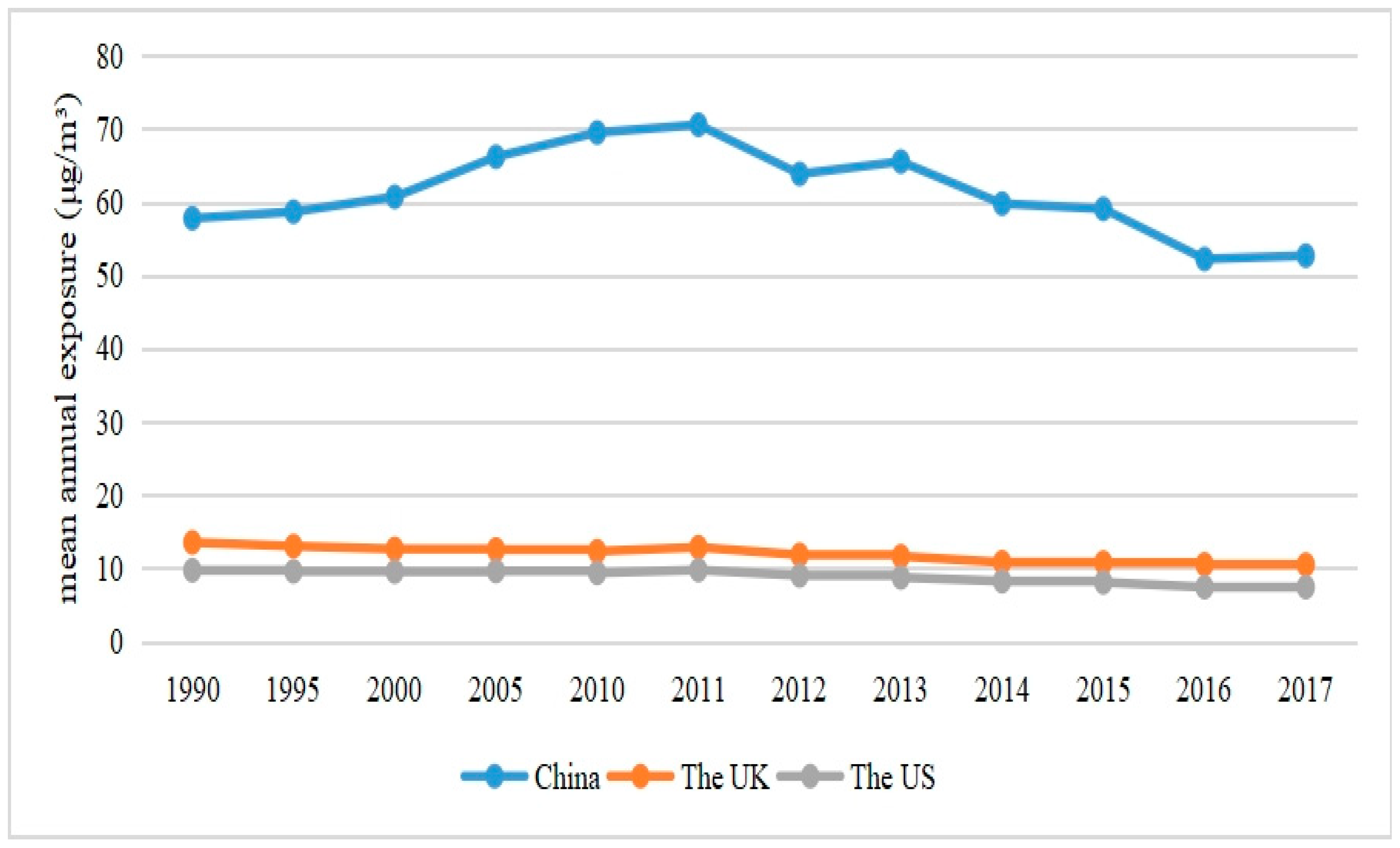
Figure 1. 1990–2017 China, the UK, and the US Population-weighted average level of exposure to PM2.5 (mean annual exposure (μg/m3)). Data source: World Bank/ourworldindata.org.
Atmosphere 13 00966 g001
Figure 2. 2006–2020 China, the UK, and the US NOx air pollution. (NOx emission metric ton/thousand people). Data source: ourworldindata.org.
Atmosphere 13 00966 g002
Figure 3. 2006–2020 China, the UK, and the US SO2 air pollution (SO2 emission metric ton/thousand people). Data source: ourworldindata.org.
Atmosphere 13 00966 g003
Figure 4. Route map of the industrial agglomeration effects on the atmospheric environment.
Atmosphere 13 00966 g004
Figure 5. Distribution of PM2.5 in different provinces of China from 2006 to 2019.
Atmosphere 13 00966 g005
Figure 6. Distribution of SO2 in Chinese provinces from 2006 to 2019.
Atmosphere 13 00966 g006
Figure 7. Distribution of NOx in Chinese provinces from 2006 to 2019 (Note: Figure 5, Figure 6 and Figure 7 are plotted by the authors using the open-source software QGIS, which is permitted for free academic use under its protocol of usage; the data contained in the maps are public data from the China Statistical Yearbook on Environment).
Atmosphere 13 00966 g007
Figure 8. Distribution of manufacturing agglomeration in different provinces of China from 2006 to 2019.
Atmosphere 13 00966 g008
Figure 9. Distribution of producer services agglomeration in different provinces of China from 2006 to 2019.
Atmosphere 13 00966 g009
Figure 10. Distribution of collaborative agglomeration in different provinces of China from 2006 to 2019. (Note: Figure 8, Figure 9 and Figure 10 are plotted by the authors using the open-source software QGIS, which is permitted for free academic use under its protocol of usage; the data contained in the maps are public data from the Statistical Yearbook of Chinese Provinces).
Atmosphere 13 00966 g010
Table 1. Data sources of all variables.
Variable TypeVariable NameIndicatorsData Source
Explained variablesPM2.5Annual average PM2.5 concentrationChina Environmental Yearbook
SO2Average annual emissions (ten thousand tons)
NOxAverage annual emissions (ten thousand tons)
Core explanatory variablesManufacturing agglomeration%Statistical Yearbook of Chinese Provinces
Producer services agglomeration%
Collaborative agglomeration%
Intermediate variablesEnergy consumption structureRatio of coal consumption to total energy consumptionChina Energy Statistical Yearbook
Human capitalRatio of R&D personnel to total employeesChina Statistical Yearbook
Control variablesEnvironmental regulationProportion of pollution controlChina Environmental Statistics Yearbook & China Statistical Yearbook
R&D intensityR&D investment intensityChina Statistical Yearbook of Science and Technology
Industrial structureProportion of secondary industry in tertiary industryCSMAR
GDP per capitaReal GDP per capitaChina Statistical Yearbook
GDP per capita squaredReal GDP per capita squared
FDI stockShare of FDI stock in GDP
OpenForeign trade dependenceCSMAR
CityProportion of urban populationNOAA/NGDC
Table 2. Descriptive statistics of all variables.
VariableObsMeanStd. Dev.MinMaxUnit
Magg4061.1040.2130.7232.040%
Sagg4061.0240.1100.7561.528%
Cagg4060.9160.0710.6370.999%
SO240659.81043.9400.190196.200ten thousand tons
NOx40659.55539.0344.000180.113ten thousand tons
PM2.540642.52213.80716.09085.628µg/m3
ER4060.0110.0140.0010.224%
RDintensity4061.5751.0930.2006.310%
INS4061.0960.3560.1932.001%
lnpergdp40610.3140.5578.64611.685Yuan
lnpergdp2406106.70811.48774.760136.540%
fcp4060.1780.1360.0050.672%
open4060.2950.3240.0281.668%
city40654.86313.72427.46089.600%
Energy4060.9630.421−0.5912.460%
RDhuman4060.0120.0080.0000.054%
Table 3. Baseline regression of the effect of the agglomeration of manufacturing on air pollution.
OLS+FEFGLSOLS+FEFGLSOLS+FEFGLS
PM2.5PM2.5NOxNOxSO2SO2
Magg6.985 **4.588 **4.8991.38433.033 *7.992 *
(3.106)(1.984)(9.608)(4.035)(19.226)(4.680)
ER−0.624−1.860−15.6809.3030.208−0.589
(13.147)(7.507)(52.543)(15.663)(57.342)(22.277)
RDintensity−0.132−1.063−0.534−0.306−5.784−4.097
(1.404)(1.141)(3.620)(2.168)(5.301)(2.693)
INS−1.6101.0304.665−2.7219.4962.628
(2.659)(1.467)(9.664)(3.655)(10.379)(3.899)
lnpergdp80.641 **43.103 **62.118145.871 **145.149143.477 **
(36.389)(17.992)(103.261)(59.627)(227.332)(70.027)
lnpergdp2−3.948 **−2.133 **−1.695−6.394 **−5.065−6.565 *
(1.855)(0.897)(4.972)(2.899)(10.842)(3.435)
fcp−16.433−10.172*−19.181−22.876−82.026−71.732 ***
(9.699)(5.892)(26.063)(16.281)(55.893)(22.241)
open−2.849−2.80628.008*9.245−2.4250.160
(4.526)(2.767)(14.797)(7.698)(27.561)(8.119)
city−0.151−0.148−0.755−0.092−4.090 ***−1.948 ***
(0.295)(0.150)(0.649)(0.355)(0.837)(0.410)
_cons−357.061 *−149.091 *−371.588−785.371 ***−669.565−530.539
(179.709)(87.636)(526.066)(291.978)(1164.765)(343.105)
N406406406406406406
R20.714 0.626 0.782
timeYesYesYesYesYesYes
ind Yes Yes Yes
Note: ① ***, **, * denote significance levels of 1%, 5%, and 10%, respectively; values in square brackets below the coefficients are robust standard errors; FE denote fixed-effect models. ② “time” represents time-fixed effects. ③ “ind” represent individual fixed effects.
Table 4. Baseline regression of the effect of the agglomeration of producer services on air pollution.
OLS+FEFGLSOLS+FEFGLSOLS+FEFGLS
PM2.5PM2.5NOxNOxSO2SO2
Sagg−5.632−9.140 **27.46914.527 *11.314−1.011
(8.697)(4.036)(19.654)(8.555)(44.863)(10.052)
ER1.400−1.265−19.3897.9553.584−1.687
(12.827)(7.519)(56.295)(15.339)(63.058)(22.339)
RDintensity−0.387−0.891−2.681−0.602−9.366−3.783
(1.783)(1.146)(4.070)(2.137)(6.241)(2.694)
INS−1.5141.1797.108−2.33112.8212.715
(2.651)(1.478)(9.652)(3.577)(11.385)(3.922)
lnpergdp81.902 **46.780 **37.861139.458 **120.747147.614 **
(38.966)(18.469)(102.611)(59.143)(240.403)(70.425)
lnpergdp2−4.082 **−2.359 **−0.582−6.080 **−4.241−6.855 **
(1.948)(0.920)(5.026)(2.877)(11.486)(3.452)
fcp−17.486 *−10.144 *−22.080−22.395−89.614−71.197 ***
(9.963)(6.016)(25.679)(16.256)(60.963)(22.172)
open−2.788−3.09628.806*9.346−1.2220.237
(4.690)(2.820)(15.143)(7.627)(28.468)(8.118)
city−0.087−0.070−0.850−0.151−3.955 ***−1.891 ***
(0.306)(0.153)(0.619)(0.349)(0.896)(0.412)
_cons−346.198 *−154.554 *−260.854−763.354 ***−493.653−539.332
(197.327)(89.571)(510.347)(288.618)(1225.996)(345.034)
N406406406406406406
R20.709 0.630 0.776
timeYesYesYesYesYesYes
ind Yes Yes Yes
Note: ① ***, **, * denote significance levels of 1%, 5%, and 10%, respectively; values in square brackets below the coefficients are robust standard errors; FE denote fixed-effect models. ② “time” represents time-fixed effects. ③ “ind” represents individual fixed effects.
Table 5. Baseline regression of the effect of co-agglomeration on air pollution.
OLS+FEFGLSOLS+FEFGLSOLS+FEFGLS
PM2.5PM2.5NOxNOxSO2SO2
Cagg−14.455 *−9.071**9.694−0.952−32.474−5.527
(7.305)(4.538)(28.569)(10.422)(54.422)(11.594)
ER−0.301−1.592−14.3819.3443.676−1.378
(12.894)(7.350)(53.591)(15.685)(59.568)(22.148)
RDintensity−0.623−1.138−1.039−0.333−8.395−3.657
(1.377)(1.139)(3.845)(2.184)(6.763)(2.675)
INS−0.7841.2944.827−2.72812.6492.722
(2.797)(1.478)(9.566)(3.657)(11.345)(3.946)
lnpergdp62.974 *34.472 *69.513144.021 **97.403143.424 **
(33.439)(18.272)(102.361)(60.584)(241.959)(71.386)
lnpergdp2−3.124 *−1.753 *−2.135−6.312 **−3.010−6.669 *
(1.665)(0.914)(4.890)(2.949)(11.592)(3.501)
fcp−14.466−10.166*−22.476−23.192−81.182−70.156 ***
(9.298)(5.991)(28.146)(16.431)(60.544)(22.300)
open−2.476−2.15528.028*9.624−1.098−0.088
(4.796)(2.796)(14.499)(7.719)(28.720)(8.150)
city−0.150−0.103−0.702−0.075−3.990***−1.872 ***
(0.269)(0.149)(0.653)(0.353)(0.950)(0.414)
_cons−243.949−92.953−407.181−774.714 ***−342.603−514.180
(169.460)(89.177)(523.263)(298.283)(1261.598)(351.630)
N406406406406406406
R20.714 0.626 0.777
timeYesYesYesYesYesYes
ind Yes Yes Yes
Note: ① ***, **, * denote significance levels of 1%,5%, and 10%, respectively; values in square brackets below the coefficients are robust standard errors; FE denote fixed-effect models. ② “time” represents time-fixed effects. ③ “ind” represents individual fixed effects.
Table 6. Regression results of the effects of the agglomeration of manufacturing, the agglomeration of producer services, and the co-agglomeration on air pollution by regions.
Eastern ChinaCentral and Western ChinaEastern ChinaCentral and Western ChinaEastern ChinaCentral and Western China
PM2.5PM2.5NOxNOxSO2SO2
Magg1.3526.208 ***1.683−0.36922.176 **6.461
(3.290)(2.269)(5.525)(6.670)(9.396)(5.964)
Sagg−9.249−12.662 ***−13.01021.519 **−38.008 *4.796
(7.555)(4.107)(18.336)(10.820)(23.065)(11.601)
Cagg−1.105−11.606 **6.01612.15117.978−19.301
(8.484)(4.931)(14.671)(15.745)(22.713)(13.892)
ControlYesYesYesYesYesYes
timeYesYesYesYesYesYes
indYesYesYesYesYesYes
N168238168238168238
Note: ① ***, **, * denote significance levels of 1%, 5%, and 10%, respectively; values in square brackets below the coefficients are robust standard errors. ② “time” represents time-fixed effects. ③ “ind” represents individual fixed effects.
Table 7. Regression of the effect of the heterogeneity of industrial agglomeration on air pollution by regions.
Eastern ChinaCentral and Western ChinaEastern ChinaCentral and Western ChinaEastern ChinaCentral and Western China
PM2.5PM2.5NOxNOxSO2SO2
Mrdi37.159 ***15.127 ***79.980 ***1.10333.075 **−11.532 *
(5.687)(3.463)(14.082)(7.377)(15.768)(6.516)
Mcom−14.525 ***−5.198 ***−31.503 ***1.637−13.976 **2.712
(2.388)(1.425)(6.134)(3.096)(6.774)(2.808)
Srdi17.280 **3.1666.873−1.1579.418−0.903
(7.705)(4.111)(19.117)(7.142)(13.550)(6.787)
Scom−57.070 ***−0.243−116.603 ***4.265−79.167 ***−6.355
(10.738)(3.275)(30.536)(7.807)(27.396)(6.580)
ControlYesYesYesYesYesYes
timeYesYesYesYesYesYes
indYesYesYesYesYesYes
N168238168238168238
Note: ① ***, **, * denote significance levels of 1%, 5%, and 10%, respectively; values in square brackets below the coefficients are robust standard errors. ② “time” represents time-fixed effects. ③ “ind” represents individual fixed effects.
Table 8. First-phase lag test of the effect of industrial agglomeration on air pollutants.
(1)(2)(3)
SO2NOxPM2.5
LMagg5.0925.4475.256 **
(5.188)(4.084)(2.135)
LSagg−2.9343.301−7.342 *
(10.706)(8.960)(4.111)
LCagg3.364−2.642−9.517 **
(12.817)(10.719)(4.750)
ControlYesYesYes
timeYesYesYes
indYesYesYes
N377377377
Note: ① **, * denote significance levels of 1%, 5%, and 10%, respectively; values in square brackets below the coefficients are robust standard errors. ② “time” represents time-fixed effects. ③ “ind” represents individual fixed effects.
Table 9. Moran index of PM2.5, NOx, SO2 emissions for 29 provinces in China, 2006–2019.
YearPM2.5NOxSO2
Moran’Ip-ValueMoran’Ip-ValueMoran’Ip-Value
20060.1350.0000.0320.050−0.0150.562
20070.1280.000−0.0150.565−0.0160.581
20080.1200.0000.0110.174−0.0160.580
20090.1350.0000.0100.181−0.0170.590
20100.1400.0000.0100.185−0.0170.588
20110.1180.0000.0290.0590.0110.167
20120.0910.0000.0280.0630.0110.171
20130.1210.0000.0260.0700.0120.158
20140.1430.0000.0250.0740.0110.170
20150.1550.0000.0230.0840.0110.169
20160.1470.000−0.0120.484−0.0140.539
20170.1340.000−0.0090.427−0.0320.915
20180.1200.0000.0010.280−0.0340.978
20190.1120.000−0.0010.313−0.0350.991
Table 10. Spatial econometric regression results in the effect of industrial agglomeration on air pollution.
(1)(2)(3)
SDMSDMSDM
Magg6.445 **
(3.036)
Sagg −8.595 *
(5.010)
Cagg −13.92 **
(7.099)
ER2.2564.3321.196
(15.10)(9.726)(14.73)
RDintensity0.471−0.672−0.218
(1.381)(1.738)(1.292)
INS−5.775 **−0.654−5.188 *
(2.550)(2.238)(2.914)
lnpergdp124.9 ***75.70 **112.3 ***
(36.77)(35.71)(35.40)
lnpergdp2−6.064 ***−3.832 **−5.458 ***
(1.771)(1.749)(1.678)
fcp−20.69 **−20.93 **−18.92 **
(8.800)(9.510)(8.603)
open−9.397 *−1.656−9.093 *
(4.802)(4.628)(5.106)
city−0.04310.0398−0.0432
(0.221)(0.241)(0.206)
Note: ***, **, * denote significance levels of 1%, 5%, and 10%, respectively; values in square brackets below the coefficients are robust standard errors.
Table 11. Instrumental variable test of the effect of industrial agglomeration on air pollutants.
(1)(2)(3)(4)(5)(6)(7)(8)(9)
PM2.5NOxSO2PM2.5NOxSO2PM2.5NOxSO2
Magg152.499 *158.487−56.902
(79.780)(108.735)(130.843)
Sagg −188.565 **−195.96970.360
(74.064)(122.180)(161.078)
Cagg −579.759 ***−609.259 **−175.468
(189.101)(260.072)(162.490)
ControlYesYesYesYesYesYesYesYesYes
timeYesYesYesYesYesYesYesYesYes
indYesYesYesYesYesYesYesYesYes
N406406406406406406406406406
Note: ① ***, **, * denote significance levels of 1%, 5%, and 10%, respectively; values in square brackets below the coefficients are robust standard error; ② “time” represents time-fixed effects. ③ “ind” represents individual fixed effects.
Table 12. Test of the mediating role of energy consumption structure in the agglomeration of manufacturing.
(1)(2)(3)(4)
EnergyPM2.5NOxSO2
Magg0.249 *5.805 *6.92834.766 *
(0.128)(2.968)(9.771)(18.511)
Energy 4.740*−8.147−6.956
(2.563)(6.426)(13.944)
ControlYesYesYesYes
timeYesYesYesYes
indYesYesYesYes
N406406406406
Note: ① * denote significance levels of 1%, 5%, and 10%, respectively; values in square brackets below the coefficients are robust standard errors. ② “time” represents time-fixed effects. ③ “ind” represents individual fixed effects.
Table 13. Test of the mediating role of energy consumption structure in the agglomeration of producer services.
(1)(2)(3)(4)
EnergyPM2.5NOxSO2
Sagg0.227−6.86329.35612.274
(0.288)(8.529)(19.086)(44.597)
Energy 5.434 *−8.332−4.239
(2.673)(6.039)(14.744)
ControlYesYesYesYes
timeYesYesYesYes
indYesYesYesYes
N406406406406
Note: ① * denote significance levels of 10%, respectively; values in square brackets below the coefficients are robust standard errors. ② “time” represents time-fixed effects. ③ “ind” represent individual fixed effects.
Table 14. Test of the mediating role of energy consumption structure in co-agglomeration.
(1)(2)(3)(4)
EnergyPM2.5NOxSO2
Cagg−1.078 ***−9.6131.712−40.089
(0.275)(6.952)(30.476)(56.803)
Energy 4.492 *−7.405−7.064
(2.583)(6.764)(15.187)
ControlYesYesYesYes
timeYesYesYesYes
indYesYesYesYes
N406406406406
Note: ① ***, * denote significance levels of 1% and 10%, respectively; values in square brackets below the coefficients are robust standard errors. ② “time” represents time-fixed effects. ③ “ind” represents individual fixed effects.
Table 15. Test of the mediating role of human capital in the agglomeration of manufacturing.
(1)(2)(3)(4)
RDhumanPM2.5NOxSO2
Magg−0.002 *3.862 **1.3167.518
(0.001)(1.939)(4.063)(4.694)
RDhuman −170.193 ***−193.257−65.690
(57.486)(156.454)(143.192)
ControlYesYesYesYes
timeYesYesYesYes
indYesYesYesYes
N406406406406
Note: ① ***, **, * denote significance levels of 1%, 5%, and 10%, respectively; values in square brackets below the coefficients are robust standard errors. ② “time” represents time-fixed effects. ③ “ind” represents individual fixed effects.
Table 16. Test of the mediating role of human capital in the agglomeration of the producer.
(1)(2)(3)(4)
RDhumanPM2.5NOxSO2
Sagg0.005 **−8.478 **15.267 *−2.180
(0.002)(3.948)(8.592)(10.210)
RDhuman −176.616 ***−202.163−64.309
(56.690)(155.538)(144.712)
ControlYesYesYesYes
timeYesYesYesYes
indYesYesYesYes
N406406406406
Note: ① ***, **, * denote significance levels of 1%,5%, and 10%, respectively; values in square brackets below the coefficients are robust standard errors. ② “time” represents time-fixed effects. ③ “ind” represent individual fixed effects.
Table 17. Test of the mediating role of human capital in co-agglomeration.
(1)(2)(3)(4)
RDhumanPM2.5NOxSO2
Cagg0.004−8.843 **−0.402−4.277
(0.003)(4.438)(10.494)(11.607)
RDhuman −175.759 ***−193.447−65.051
(57.768)(156.631)(143.488)
ControlYesYesYesYes
timeYesYesYesYes
indYesYesYesYes
N406406406406
Note: ① ***, ** denote significance levels of 1% and 5%, respectively; values in square brackets below the coefficients are robust standard errors. ② “time” represents time-fixed effects. ③ “ind” represents individual fixed effects.
Publisher’s Note: MDPI stays neutral with regard to jurisdictional claims in published maps and institutional affiliations.