
Impacts of the Thermal Gradient on Inland Advecting Sea Breezes in the Southeastern United States


Abstract
:1. Introduction
2. Methods
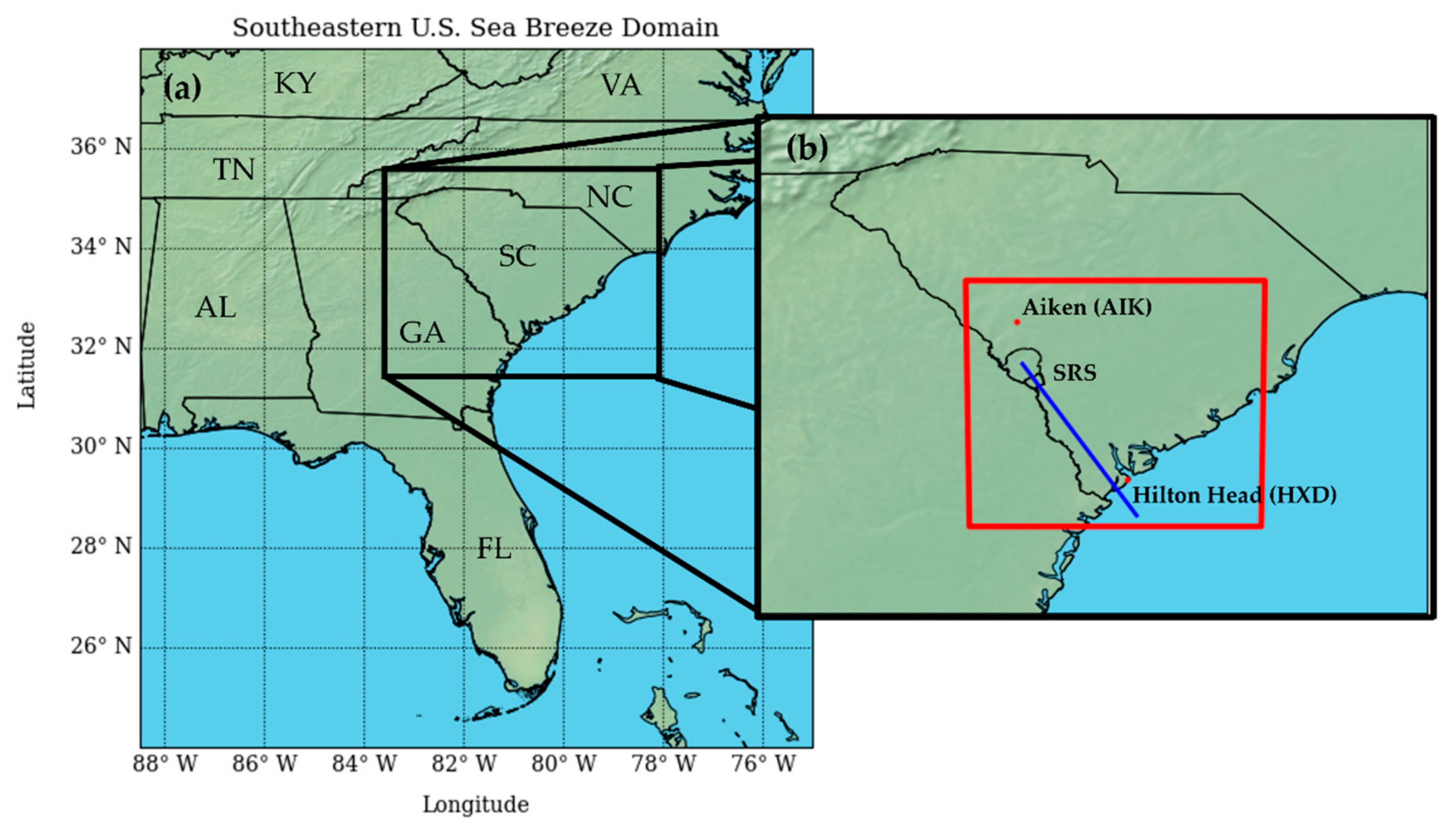
2.1. Observations
2.2. WRF Model Setup
3. Results
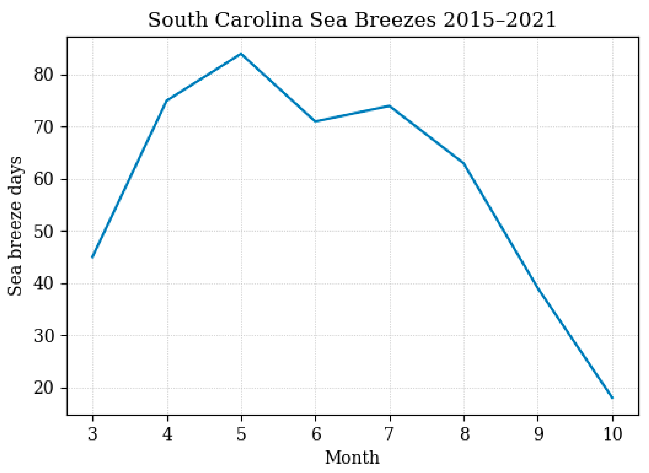
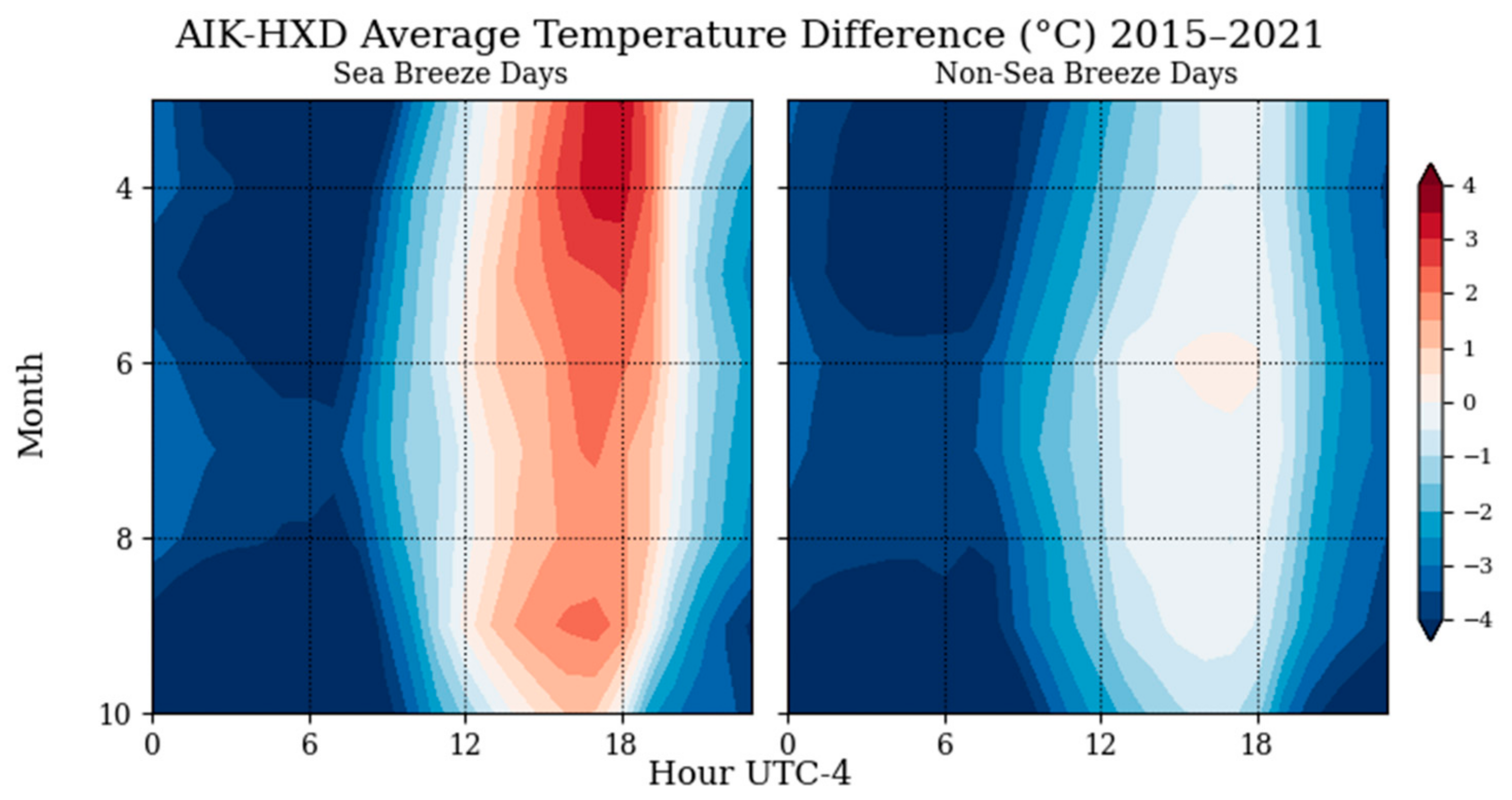
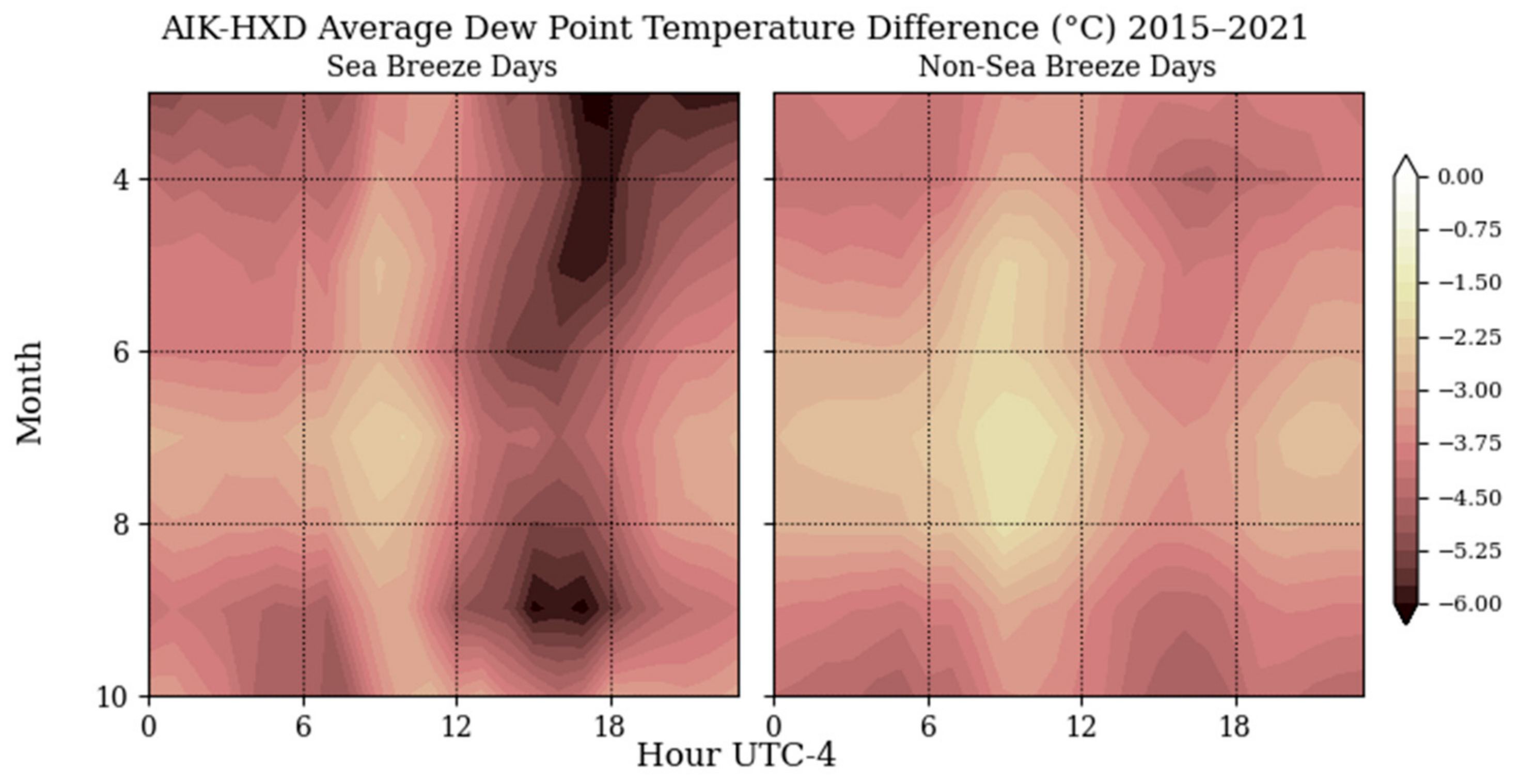
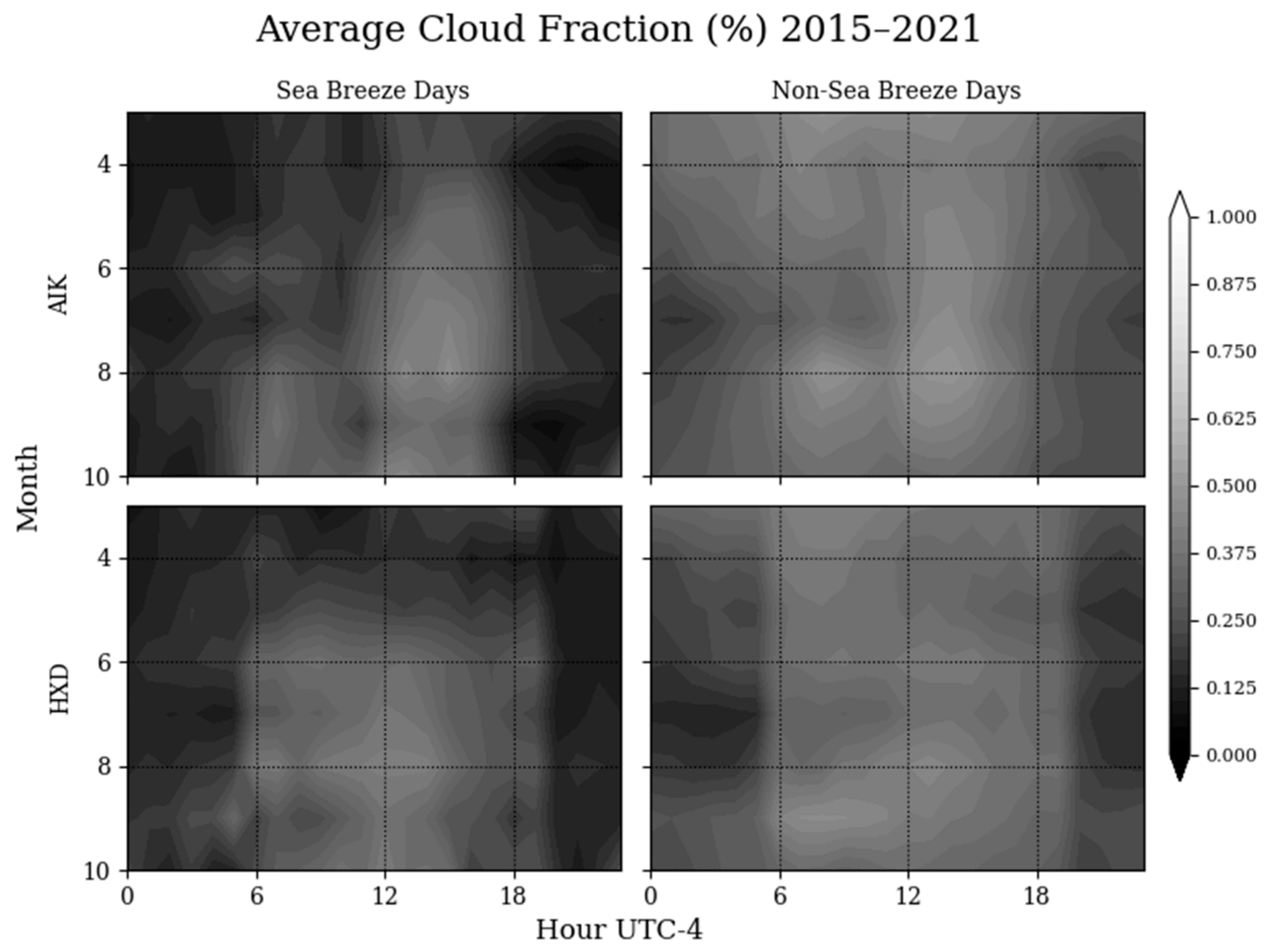
3.1. Observed Results
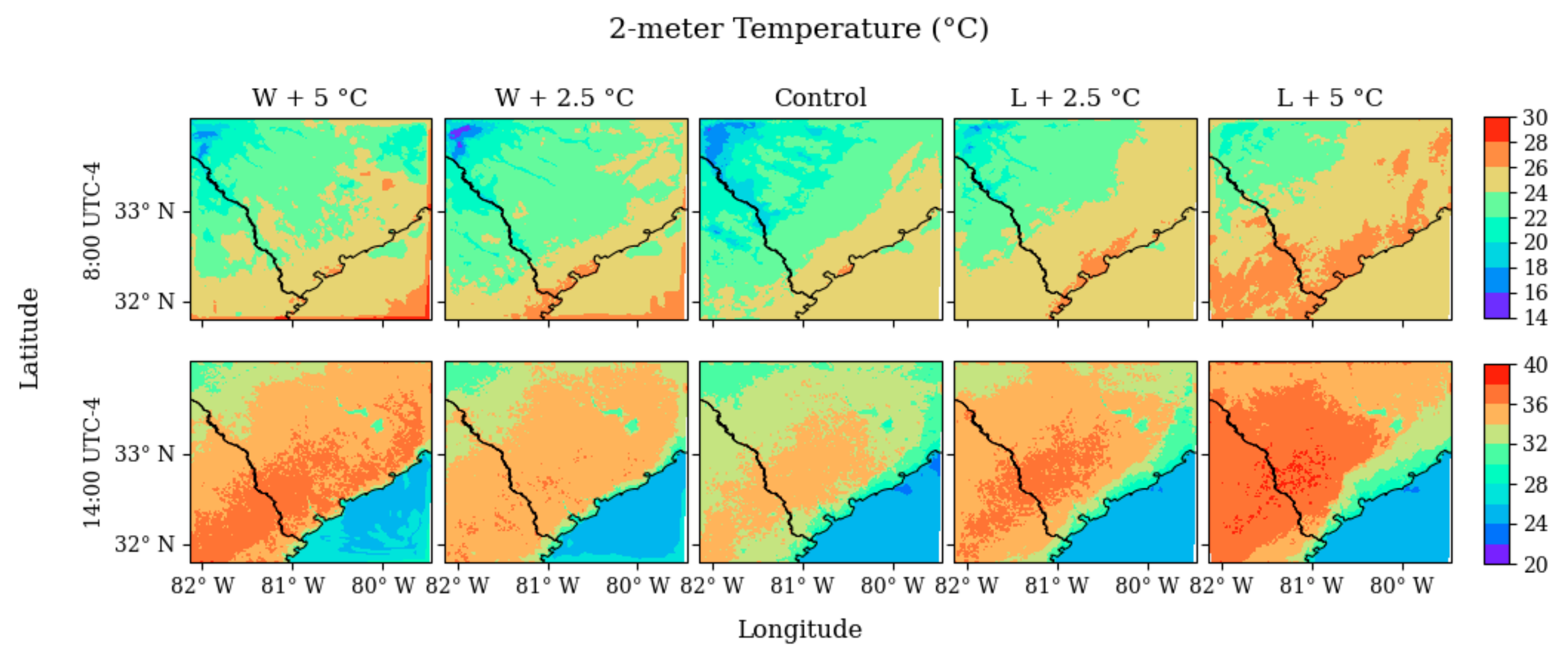
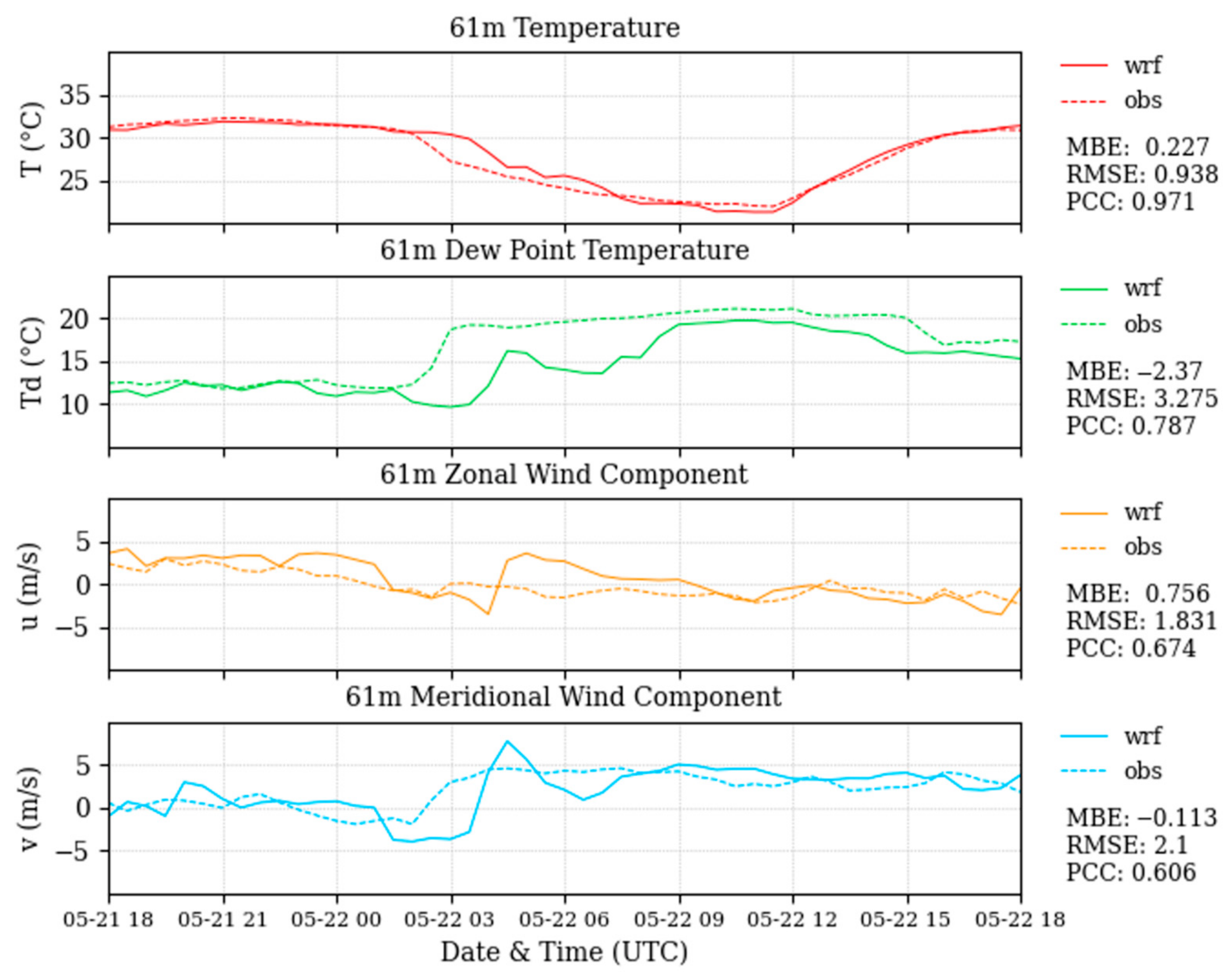
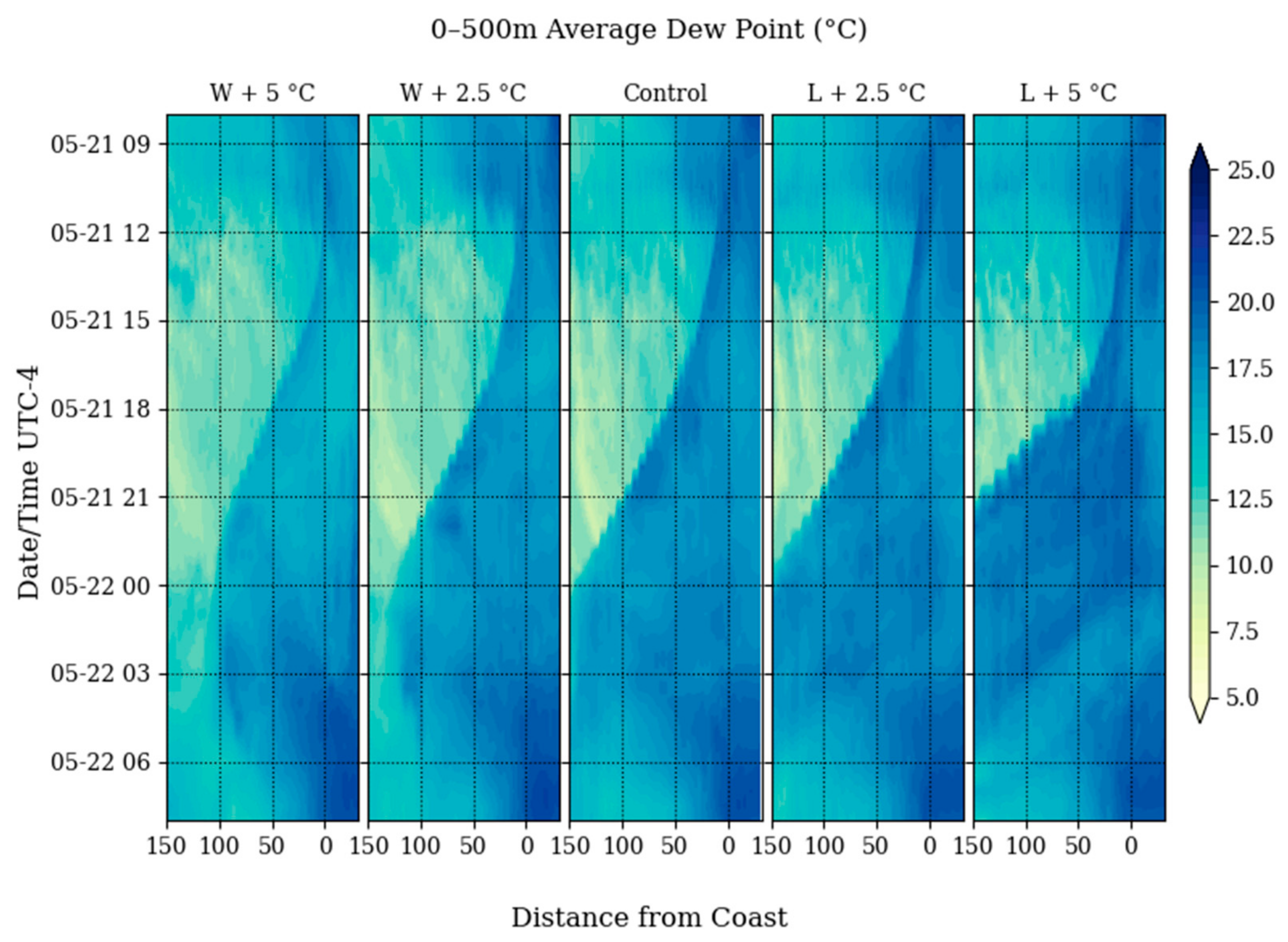
3.2. WRF Simulation Results
4. Conclusions
Author Contributions
Funding
Institutional Review Board Statement
Informed Consent Statement
Data Availability Statement
Acknowledgments
Conflicts of Interest
References
- Case, J.L.; Wheeler, M.M.; Manobianco, J.; Weems, J.W.; Roeder, W.P. A 7-yr climatological study of land breezes over the Florida spaceport. J. Appl. Meteorol. 2005, 44, 340–356. [Google Scholar] [CrossRef] [Green Version]
- Hill, C.M.; Fitzpatrick, P.J.; Corbin, J.H.; Lau, Y.H.; Bhate, S.K. Summertime Precipitation Regimes Associated with the Sea Breeze and Land Breeze in Southern Mississippi and Eastern Louisiana. Weather. Forecast. 2010, 25, 1755–1779. [Google Scholar] [CrossRef]
- White, L.D.; Koziara, M. Surface Thermodynamic Gradients Associated with Gulf of Mexico Sea-Breeze Fronts. Adv. Meteorol. 2018, 2018, 2601346. [Google Scholar] [CrossRef]
- Buckley, R.L.; Kurzeja, R.J. An observational and numerical study of the nocturnal sea breeze. Part I: Structure and circulation. J. Appl. Meteorol. 1997, 36, 1577–1598. [Google Scholar] [CrossRef]
- Miller, S.T.K.; Keim, B.D.; Talbot, R.W.; Mao, H. Sea breeze: Structure, forecasting, and impacts. Rev. Geophys. 2003, 41, 1011. [Google Scholar] [CrossRef] [Green Version]
- Melas, D.; Lavagnini, A.; Sempreviva, A.M. An investigation of the boundary layer dynamics of Sardinia Island under sea-breeze conditions. J. Appl. Meteorol. 2000, 39, 516–524. [Google Scholar] [CrossRef]
- Qian, T.T.; Epifanio, C.C.; Zhang, F.Q. Topographic Effects on the Tropical Land and Sea Breeze. J. Atmos. Sci. 2012, 69, 130–149. [Google Scholar] [CrossRef] [Green Version]
- Rotunno, R. On the Linear-Theory of the Land and Sea Breeze. J. Atmos. Sci. 1983, 40, 1999–2009. [Google Scholar] [CrossRef]
- Steele, C.J.; Dorling, S.R.; von Glasow, R.; Bacon, J. Modelling sea-breeze climatologies and interactions on coasts in the southern North Sea: Implications for offshore wind energy. Q. J. R. Meteorol. Soc. 2015, 141, 1821–1835. [Google Scholar] [CrossRef] [Green Version]
- Shepherd, J.M.; Carter, W.M.; Manyin, M.; Messen, D.; Burian, S. The impact of urbanization on current and future coastal convection: A case study for Houston. Environ. Plan. 2010, 37, 284–304. [Google Scholar] [CrossRef] [Green Version]
- Simpson, J.E.; Mansfield, D.A.; Milford, J.R. Inland Penetration of Sea-Breeze Fronts. Q. J. R. Meteorol. Soc. 1977, 103, 47–76. [Google Scholar] [CrossRef]
- Muppa, S.K.; Anandan, V.K.; Kesarkar, K.A.; Rao, S.V.B.; Reddy, P.N. Study on deep inland penetration of sea breeze over complex terrain in the tropics. Atmos. Res. 2012, 104, 209–216. [Google Scholar] [CrossRef]
- Viner, B.; Noble, S.; Qian, J.H.; Werth, D.; Gayes, P.; Pietrafesa, L.; Bao, S.W. Frequency and Characteristics of Inland Advecting Sea Breezes in the Southeast United States. Atmosphere 2021, 12, 950. [Google Scholar] [CrossRef]
- Banta, R.M. Sea Breezes Shallow and Deep on the California Coast. Mon. Weather Rev. 1995, 123, 3614–3622. [Google Scholar] [CrossRef] [Green Version]
- Wagner, N.L.; Riedel, T.P.; Roberts, J.M.; Thornton, J.A.; Angevine, W.M.; Williams, E.J.; Lerner, B.M.; Vlasenko, A.; Li, S.M.; Dube, W.P.; et al. The sea breeze/land breeze circulation in Los Angeles and its influence on nitryl chloride production in this region. J. Geophys. Res. Atmos. 2012, 117, D00V24. [Google Scholar] [CrossRef]
- Arritt, R.W. Effects of the Large-Scale Flow on Characteristic Features of the Sea Breeze. J. Appl. Meteorol. 1993, 32, 116–125. [Google Scholar] [CrossRef] [Green Version]
- Skamarock, W.C.; Klemp, J.B.; Dudhia, J.; Gill, D.O.; Liu, Z.; Berner, J.; Wang, W.; Powers, J.G.; Duda, M.G.; Barker, D.M.; et al. A Description of the Advanced Research WRF Version 4; National Center for Atmospheric Research: Boulder, CO, USA, 2019; p. 145. [Google Scholar] [CrossRef]
- Weinbeck, S.; Viner, B.; Rivera-Giboyeaux, A. Meteorological Monitoring Program at the Savannah River Site; Savannah River National Laboratory: Jackson, SC, USA, 2020. [Google Scholar]
- Qian, J.H.; Viner, B.; Noble, S.; Werth, D. Precipitation Characteristics of Warm Season Weather Types in the Southeastern United States of America. Atmosphere 2021, 12, 1001. [Google Scholar] [CrossRef]
- Benjamin, S.G.; Weygandt, S.S.; Brown, J.M.; Hu, M.; Alexander, C.R.; Smirnova, T.G.; Olson, J.B.; James, E.P.; Dowell, D.C.; Grell, G.A.; et al. A North American Hourly Assimilation and Model Forecast Cycle: The Rapid Refresh. Mon. Weather Rev. 2016, 144, 1669–1694. [Google Scholar] [CrossRef]
- Thompson, G.; Field, P.R.; Rasmussen, R.M.; Hall, W.D. Explicit Forecasts of Winter Precipitation Using an Improved Bulk Microphysics Scheme. Part II: Implementation of a New Snow Parameterization. Mon. Weather Rev. 2008, 136, 5095–5115. [Google Scholar] [CrossRef]
- Dudhia, J. Numerical Study of Convection Observed during the Winter Monsoon Experiment Using a Mesoscale Two-Dimensional Model. J. Atmos. Sci. 1989, 46, 3077–3107. [Google Scholar] [CrossRef]
- Mlawer, E.J.; Taubman, S.J.; Brown, P.D.; Iacono, M.J.; Clough, S.A. Radiative transfer for inhomogeneous atmospheres: RRTM, a validated correlated-k model for the longwave. J. Geophys. Res. Atmos. 1997, 102, 16663–16682. [Google Scholar] [CrossRef] [Green Version]
- Nakanishi, M.; Niino, H. Development of an Improved Turbulence Closure Model for the Atmospheric Boundary Layer. J. Meteorol. Soc. Jpn 2009, 87, 895–912. [Google Scholar] [CrossRef] [Green Version]
- Mitchell, K. The Community Noah Land-Surface Model (LSM); University Center of Atmospheric Research: Boulder, CO, USA, 2005; p. 26. [Google Scholar]
- Kusaka, H.; Kondo, H.; Kikegawa, Y.; Kimura, F. A simple single-layer urban canopy model for atmospheric models: Comparison with multi-layer and slab models. Bound Lay Meteorol. 2001, 101, 329–358. [Google Scholar] [CrossRef]
- Steele, C.J.; Dorling, S.R.; von Glasow, R.; Bacon, J. Idealized WRF model sensitivity simulations of sea breeze types and their effects on offshore windfields. Atmos. Chem. Phys. 2013, 13, 443–461. [Google Scholar] [CrossRef] [Green Version]
- Lombardo, K.; Sinsky, E.; Jia, Y.; Whitney, M.M.; Edson, J. Sensitivity of Simulated Sea Breezes to Initial Conditions in Complex Coastal Regions. Mon. Weather Rev. 2016, 144, 1299–1320. [Google Scholar] [CrossRef]
- Huang, J.H. A Simple Accurate Formula for Calculating Saturation Vapor Pressure of Water and Ice. J. Appl. Meteorol. Clim. 2018, 57, 1265–1272. [Google Scholar] [CrossRef]
- Novak, D.R.; Colle, B.A. Observations of multiple sea breeze boundaries during an unseasonably warm day in metropolitan New York City. B Am. Meteorol. Soc. 2006, 87, 169–174. [Google Scholar] [CrossRef]
- Azorin-Molina, C.; Tijm, S.; Chen, D.L. Development of selection algorithms and databases for sea breeze studies. Theor. Appl. Climatol. 2011, 106, 531–546. [Google Scholar] [CrossRef]

| Sky Condition | ASOS Code | Assigned Value |
|---|---|---|
| Clear | CLR | 0.00 |
| Few | FEW | 0.25 |
| Scattered | SCT | 0.50 |
| Broken | BKN | 0.75 |
| Overcast | OVC | 1.00 |
| Parameter | Model |
|---|---|
| Microphysics | Thompson [21] |
| Radiation | RRTM + Dudhia [22,23] |
| Surface-Layer Model | MYNN 2.5-level [24] |
| Land-Surface Model | Noah LSM [25] |
| Urban Physics | Single-Layer Urban Canopy Model [26] |
| PBL Scheme | MYNN 2.5-level [24] |
| Cumulus Parameterization | None |
Publisher’s Note: MDPI stays neutral with regard to jurisdictional claims in published maps and institutional affiliations. |
© 2022 by the authors. Licensee MDPI, Basel, Switzerland. This article is an open access article distributed under the terms and conditions of the Creative Commons Attribution (CC BY) license (https://creativecommons.org/licenses/by/4.0/).
Share and Cite
Wermter, J.; Noble, S.; Viner, B. Impacts of the Thermal Gradient on Inland Advecting Sea Breezes in the Southeastern United States. Atmosphere 2022, 13, 1004. https://doi.org/10.3390/atmos13071004
Wermter J, Noble S, Viner B. Impacts of the Thermal Gradient on Inland Advecting Sea Breezes in the Southeastern United States. Atmosphere. 2022; 13(7):1004. https://doi.org/10.3390/atmos13071004
Chicago/Turabian StyleWermter, Joseph, Stephen Noble, and Brian Viner. 2022. "Impacts of the Thermal Gradient on Inland Advecting Sea Breezes in the Southeastern United States" Atmosphere 13, no. 7: 1004. https://doi.org/10.3390/atmos13071004