
The Impact of High-Resolution SRTM Topography and Corine Land Cover on Lightning Calculations in WRF

 , , , ,
Abstract
:1. Introduction
2. Methodology
2.1. Description of WRF
2.2. Land Coverage Differences between Corine and USGS
3. Results
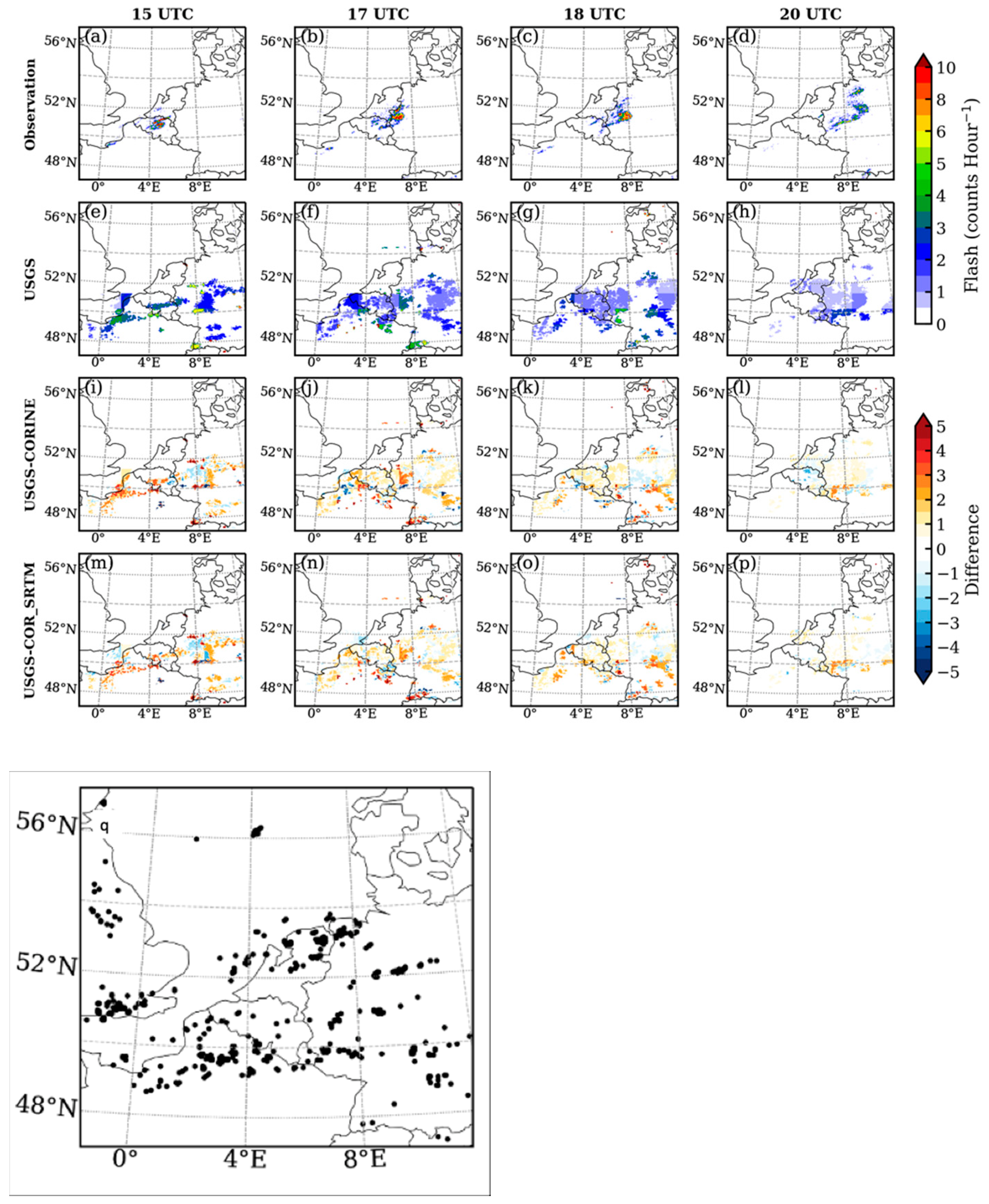
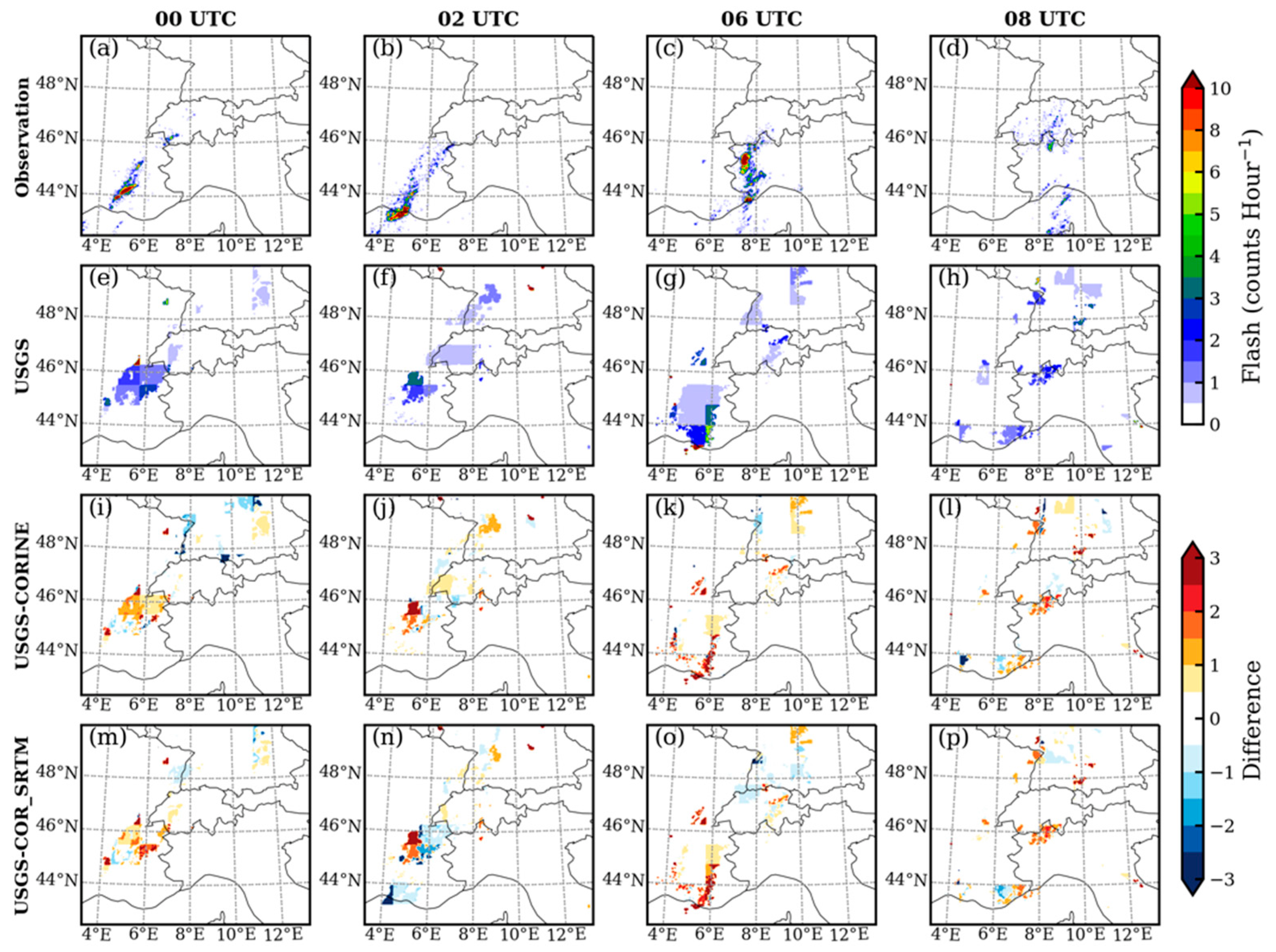
3.1. Lightning
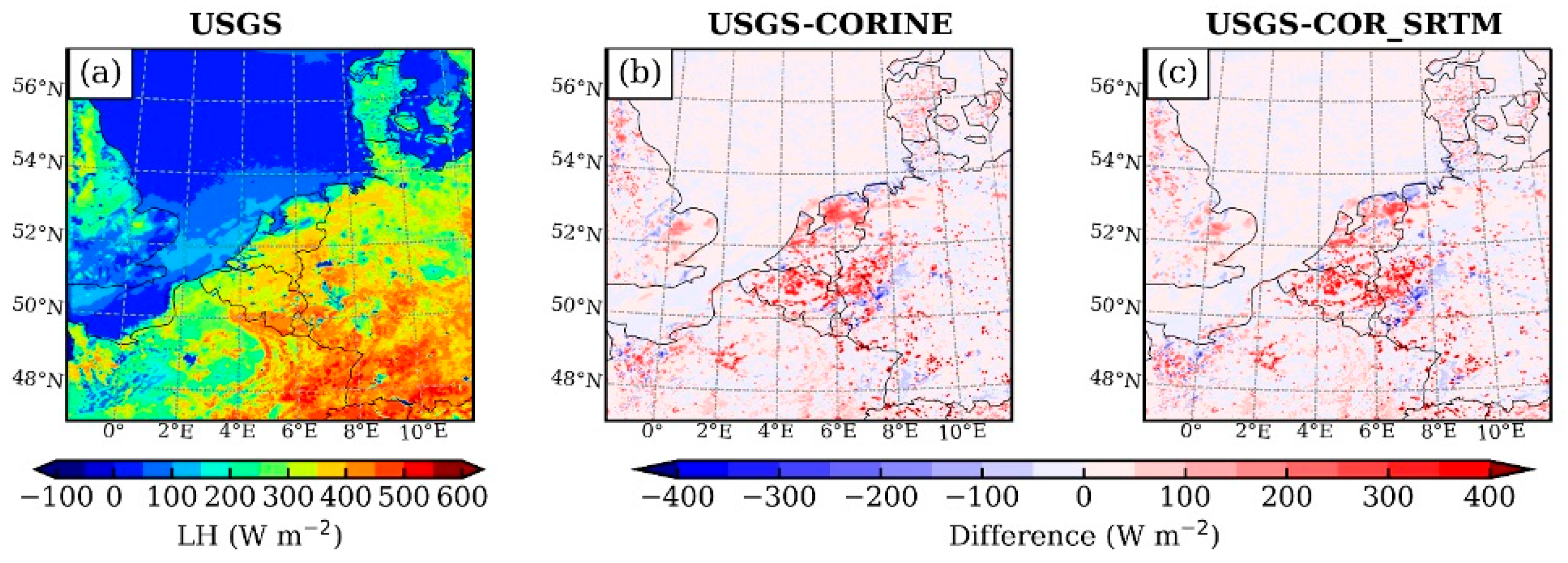
3.2. Heat Fluxes
3.3. Vertical Profiles of Model Bias
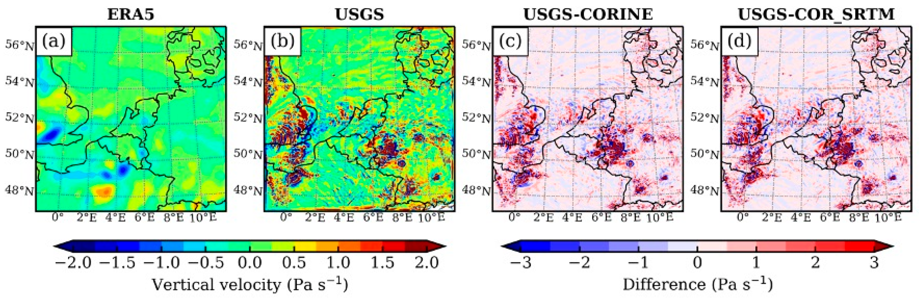
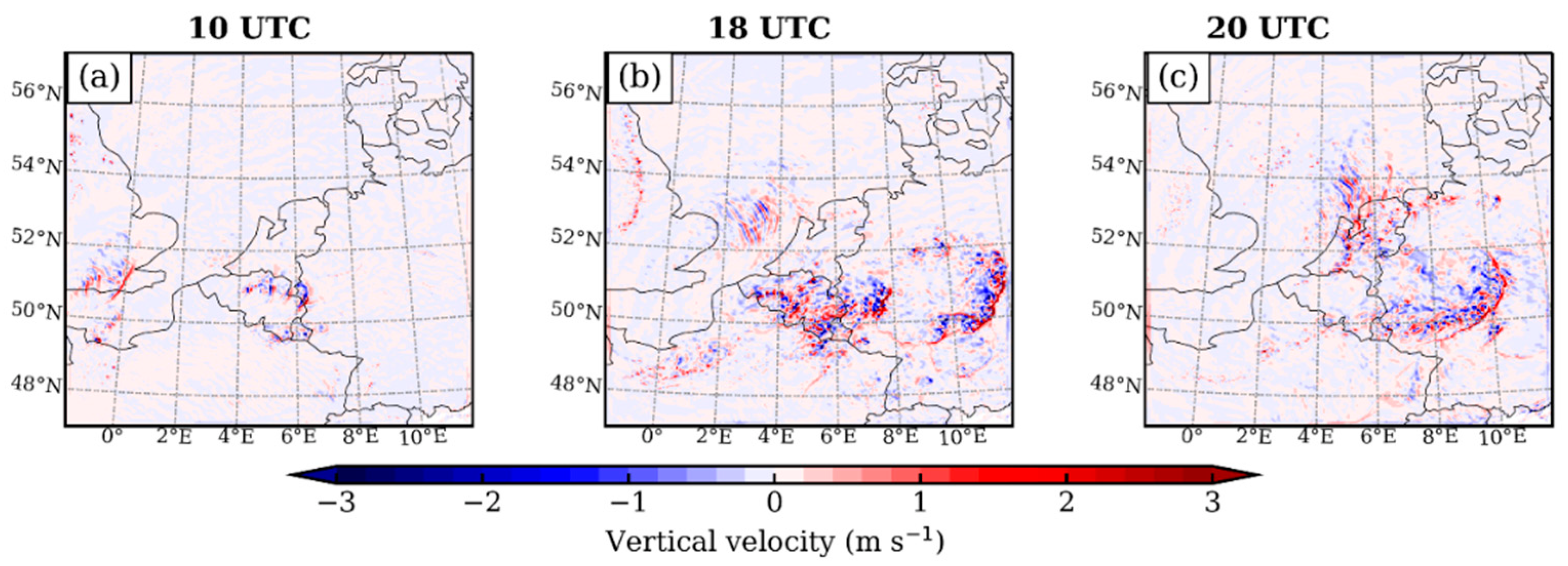
3.4. CAPE and Vertical Wind
4. Conclusions and Discussions
Author Contributions
Funding
Institutional Review Board Statement
Informed Consent Statement
Data Availability Statement
Acknowledgments
Conflicts of Interest
References
- IPCC. Climate Change 2014: Synthesis Report. Contribution of Working Groups I, II and III to the Fifth Assessment Report of the Intergovernmental Panel on Climate Change; Core Writing Team, Pachauri, R.K., Meyer, L.A., Eds.; IPCC: Geneva, Switzerland, 2014; 151p. [Google Scholar]
- Romps, D.M.; Seeley, J.T.; Vollaro, D.; Molinari, J. Projected increase in lightning strikes in the United States due to global warming. Science 2014, 346, 851–854. [Google Scholar] [CrossRef] [PubMed]
- Finney, D.L.; Doherty, R.M.; Wild, O.; Stevenson, D.S.; MacKenzie, I.A.; Blyth, A.M. A projected decrease in lightning under climate change. Nat. Clim. Chang. 2018, 8, 210–213. [Google Scholar] [CrossRef]
- Pineda, N.; Montanyà, J.; van der Velde, O.A. Characteristics of lightning related to wildfire ignitions in Catalonia. Atmospheric Res. 2014, 135–136, 380–387, ISSN 0169-8095. [Google Scholar] [CrossRef]
- Moris, J.V.; Conedera, M.; Nisi, L.; Bernardi, M.; Cesti, G.; Pezzatti, G.B. Lightning-caused fires in the Alps: Identifying the igniting strokes. Agric. For. Meteorol. 2020, 290, 107990, ISSN 0168-1923. [Google Scholar] [CrossRef]
- Pérez-Invernón, F.J.; Huntrieser, H.; Soler, S.; Gordillo-Vázquez, F.J.; Pineda, N.; Navarro-González, J.; Reglero, V.; Montanyà, J.; van der Velde, O.; Koutsias, N. Lightning-ignited wildfires and long continuing current lightning in the Mediterranean Basin: Preferential meteorological conditions. Atmos. Chem. Phys. 2021, 21, 17529–17557. [Google Scholar] [CrossRef]
- Schumann, U.; Huntrieser, H. The global lightning-induced nitrogen oxides source. Atmos. Chem. Phys. 2007, 7, 3823–3907. [Google Scholar] [CrossRef] [Green Version]
- Ryu, J.-H.; Jenkins, G. Lightning-tropospheric ozone connections: EOF analysis of TCO and lightning data. Atmos. Environ. 2005, 39, 5799–5805. [Google Scholar] [CrossRef]
- Williams, E.; Renno, N. An analysis of the conditional instability of the tropical atmosphere. Mon. Weather. Rev. 1993, 121, 21–26. [Google Scholar] [CrossRef] [Green Version]
- Moncrieff, M.W.; Miller, M.J. The dynamics and simulation of tropical cumulonimbus and squall lines. Q. J. R. Meteorol. Soc. 120 1976, 432, 373–394. [Google Scholar] [CrossRef]
- Sun, M.; Liu, D.; Qie, X.; Mansell, E.R.; Yair, Y.; Fierro, A.O.; Yuan, S.; Chen, Z.; Wang, D. Aerosol effects on electrification and lightning discharges in a multicell thunderstorm simulated by the WRF-ELEC model. Atmos. Chem. Phys. 2021, 21, 14141–14158. [Google Scholar] [CrossRef]
- Mansell, E.R.; Ziegler, C.L. Aerosol Effects on Simulated Storm Electrification and Precipitation in a Two-Moment Bulk Microphysics Model. J. Atmos. Sci. 2013, 70, 2032–2050. [Google Scholar] [CrossRef]
- Zhao, P.; Yin, Y.; Xiao, H. The effects of aerosol on development of thunderstorm electrification: A numerical study. Atmos. Res. 2015, 153, 376–391. [Google Scholar] [CrossRef]
- Jankov, I.; Gallus, W.A., Jr.; Segal, M.; Shaw, B.; Koch, S.E. The impact of Different WRF Model Physical Parameterizations and Their Interactions on Warm Season MCS Rainfall. Weather. Forecast. 2005, 20, 1048–1060. [Google Scholar] [CrossRef]
- Jankov, I.; Grasso, L.D.; Sengupta, M.; Neiman, P.J.; Zupanski, D.; Zupanski, M.; Lindsey, D.; Hillger, D.; Birkenheuer, D.L.; Brummer, R.; et al. An Evaluation of Five ARW-WRF Microphysics Schemes Using Synthetic GOES Imagery for an Atmospheric River Event Affecting the California Coast. J. Hydrometeorol. 2011, 12, 618–633. [Google Scholar] [CrossRef] [Green Version]
- Morrison, H.; Curry, J.A.; Khvorostyanov, V.I. A New Double-Moment Microphysics Parameterization for Application in Cloud and Climate Models. Part I: Decription. J. Atmos. Sci. 2005, 62, 1665–1677. [Google Scholar] [CrossRef]
- Morrison, H.; Gettelman, A. A new two-moment bulk stratiform cloud microphysics scheme in the Community Atmospheric Model (CAM3), Part I: Description and Numerical Tests. J. Clim. 2008, 21, 3642–3659. [Google Scholar] [CrossRef]
- Morrison, H.; Thompson, G.; Tatarskii, V. Impact of Cloud Microphysics on the Development of Trailing Stratiform Precipitation in a Simulated Squall Line: Comparison of One- and Two-Moment Schemes. Mon. Weather Rev. 2009, 137, 991–1007. [Google Scholar] [CrossRef] [Green Version]
- Morrison, H.; Morales, A.; Villanueva-Birriel, C. Concurrent Sensitivities of an Idealized Deep Convective Storm to Parameterization of Microphysics, Horizontal Grid Resolution, and Environmental Static Stability. Mon. Weather Rev. 2015, 143, 2082–2104. [Google Scholar] [CrossRef]
- Thompson, G.; Rasmussen, R.M.; Manning, K. Explicit Forecasts of Winter Precipitation Using an Improved Bulk Microphysics Scheme. Part I: Description and Sensitivity Analysis. Mon. Weather Rev. 2004, 132, 519–542. [Google Scholar] [CrossRef] [Green Version]
- Thompson, G.; Field, P.R.; Rasmussen, R.M.; Hall, W.D. Explicit Forecasts of winter precipitation using an improved bulk microphysics scheme. Part II: Implementation of a new snow parameterization. Mon. Weather Rev. 2008, 136, 5095–5115. [Google Scholar] [CrossRef]
- Vigaud, N.; Richard, Y.; Rouault, M.; Fauchereau, N. Moisture transport between the South Atlantic Ocean and southern Africa: Relationships with summer rainfall and associated dynamics. Clim. Dyn. 2009, 32, 113–123. [Google Scholar] [CrossRef]
- Hong, S.-Y.; Lim, K.-S.S.; Lee, Y.-H.; Ha, J.-C.; Kim, H.-W.; Ham, S.-J.; Dudhia, J. Evaluation of the WRF Double-Moment 6-Class Microphysics Scheme for Precipitating Convection. Adv. Meteorol. 2010, 2010, 707253. [Google Scholar] [CrossRef] [Green Version]
- Rajeevan, M.; Kesarkar, A.; Thampi, S.B.; Rao, T.N.; Radhakrishna, B.; Rajasekhar, M. Sensitivity of WRF cloud microphysics to simulations of a severe thunderstorm event over Southeast India. Ann. Geophys. 2010, 28, 603–619. [Google Scholar] [CrossRef]
- Pohl, B.; Crétat, J.; Camberlin, P. Testing WRF capability in simulating the atmospheric water cycle over Equatorial East Africa. Clim. Dyn. 2011, 37, 1357–1379. [Google Scholar] [CrossRef]
- Niu, G.-Y.; Yang, Z.-L.; Mitchell, K.E.; Chen, F.; Ek, M.B.; Barlage, M.; Kumar, A.; Manning, K.; Niyogi, D.; Rosero, E.; et al. The community Noah land surface model with multiparameterization options (Noah-MP): 1. Model description and evaluation with local-scale measurements. J. Geophys. Res. 2011, 116, D12109. [Google Scholar] [CrossRef] [Green Version]
- Lee, S.S.; Donner, L.J. Effects of cloud parameterization on radiation and precipitation: A comparison between single-moment microphysics and double-moment microphysics. Terr. Atmos. Ocean. Sci. 2011, 22, 403–420. [Google Scholar] [CrossRef] [Green Version]
- Molthan, A.L. Evaluating the Performance of Single and Double Moment Microphysics Schemes During a Synoptic-Scale Snowfall Event; AMS Conferences on Weather and Forecasting/Numerical Weather Prediction: Seattle, WA, USA, 2011. [Google Scholar]
- Song, X.; Zhang, G.J.; Li, J.-L.F. Evaluation of Microphysics Parameterization for Convective Clouds in the NCAR Community Atmosphere Model CAM5. J. Clim. 2012, 25, 8568–8590. [Google Scholar] [CrossRef]
- Wheatley, D.M.; Yussouf, N.; Stensrud, D.J. Ensemble Kalman Filter Analyses and Forecasts of a Severe Mesoscale Convective System Using Different Choices of Microphysics Schemes. Mon. Weather Rev. 2014, 142, 3243–3263. [Google Scholar] [CrossRef]
- Grabowski, W.W. Extracting Microphysical Impacts in Large-Eddy Simulations of Shallow Convection. J. Atmos. Sci. 2014, 71, 4493–4499. [Google Scholar] [CrossRef]
- Storer, R.L.; Zhang, G.J.; Song, X. Effects of Convective Microphysics Parameterization on Large-Scale Cloud Hydrological Cycle and Radiative Budget in Tropical and Midlatitude Convective Regions. J. Clim. 2015, 28, 9277–9297. [Google Scholar] [CrossRef]
- Min, K.-H.; Choo, S.-H.; Lee, D.-H.; Lee, G.-W. Evaluation of WRF Cloud Microphysics Schemes Using Radar Observations. Weather Forecast. 2015, 30, 1571–1589. [Google Scholar] [CrossRef]
- Pieri, A.B.; Von Hardenberg, J.; Parodi, A.; Provenzale, A. Sensitivity of Precipitation Statistics to Resolution, Microphysics, and Convective Parameterization: A Case Study with the High-Resolution WRF Climate Model over Europe. J. Hydrometeorol. 2015, 16, 1857–1872. [Google Scholar] [CrossRef]
- Halder, M.; Hazra, A.; Mukhopadhyay, P.; Siingh, D. Effect of the better representation of the cloud ice-nucleation in WRF microphysics schemes: A case study of a severe storm in India. Atmos. Res. 2015, 154, 155–174. [Google Scholar] [CrossRef]
- Khain, A.; Lynn, B.; Shpund, J. High resolution WRF simulations of Hurricane Irene: Sensitivity to aerosols and choice of microphysical schemes. Atmos. Res. 2016, 167, 129–145. [Google Scholar] [CrossRef] [Green Version]
- Bossioli, E.; Tombrou-Tzella, M.; Dandou, A.; Athanasopoulou, E.; Varotsos, K.V. The Role of Planetary Boundary-Layer Parameterizations in the Air Quality of an Urban Area with Complex Topography. Bound.-Layer Meteorol. 2009, 131, 53–72. [Google Scholar] [CrossRef]
- De Meij, A.; Gzella, A.; Cuvelier, C.; Thunis, P.; Bessagnet, B.; Vinuesa, J.F.; Menut, L.; Kelder, H.M. The impact of MM5 and WRF meteorology over complex terrain on CHIMERE model calculations. Atmos. Chem. Phys. 2009, 9, 6611–6632. [Google Scholar] [CrossRef] [Green Version]
- De Foy, B.; Lei, W.; Zavala, M.; Volkamer, R.; Samuelsson, J.; Mellqvist, J.; Galle, B.; Martínez, A.-P.; Grutter, M.; Molina, L.T. Modelling constraints on the emission inventory and on vertical diffusion for CO and SO2 in the Mexico City Metropolitan Area using Solar FTIR and zenith sky UV spectroscopy. Atmos. Chem. Phys. Discuss. 2006, 6, 6125–6181. [Google Scholar]
- Mao, Q.; Gautney, L.L.; Cook, T.M.; Jacobs, M.E.; Smith, S.N.; Kelsoe, J.J. Numerical experiments on MM5–CMAQ sensitivity to various PBL schemes. Atmos. Environ. 2006, 40, 3092–3110. [Google Scholar] [CrossRef]
- Pérez, C.; Jiménez, P.; Jorba, O.; Sicard, M.; Baldasano, J.M. Influence of the PBL scheme on high-resolution photochemical simulations in an urban coastal area over the Western Mediterranean. Atmos. Environ. 2006, 40, 5274–5297. [Google Scholar] [CrossRef]
- Lee, S.H.; Kim, S.W.; Angevine, W.; Bianco, L.; McKeen, S.; Senff, C.; Trainer, M.; Tucker, S.; Zamora, R. Evaluation of urban surface parameterizations in the WRF model using measurements during the Texas Air Quality Study 2006 field campaign. Atmos. Chem. Phys. 2010, 11, 2127–2143. [Google Scholar] [CrossRef] [Green Version]
- De Meij, A.; Vinuesa, J. Impact of SRTM and Corine Land Cover data on meteorological parameters using WRF. Atmos. Res. 2014, 143, 351–370. [Google Scholar] [CrossRef]
- Farr, T.G.; Rosen, P.A.; Caro, E.; Crippen, R.; Duren, R.; Hensley, S.; Kobrick, M.; Paller, M.; Rodriguez, E.; Roth, L.; et al. The Shuttle Radar Topography Mission. Rev. Geophys. 2007, 45, RG2004. Available online: https://agupubs.onlinelibrary.wiley.com/doi/full/10.1029/2005RG000183 (accessed on 25 April 2022). [CrossRef] [Green Version]
- Heymann, Y.; Steenmans, C.; Croissille, G.; Bossard, M. CORINE Land Cover. In Technical Guide; EUR12585; Office for Official Publications of the European Communities: Luxembourg, 1994. [Google Scholar]
- Büttner, G.; Feranec, J.; Jaffrain, G.; Mari, L.; Maucha, G.; Soukup, T. The European CORINE Land Cover Database. In Proceedings of the ISPRS Commission VII Symposium, Budapest, Hungary, 1–4 September 1998; pp. 633–638. [Google Scholar]
- Büttner, G.; Feranec, G.; Jaffrain, G. Corine Land Cover Update 2000, Technical Guidelines. EEA Technical Report No 89. 2002. Available online: http://reports.eea.europa.eu/technical_report_2002_89/en (accessed on 25 April 2022).
- Weather Research and Forecasting Model. Available online: https://www.mmm.ucar.edu/weather-research-and-forecasting-model (accessed on 25 April 2022).
- Skamarock, W.C.; Klemp, J.B.; Dudhia, J.; Gill, D.O.; Liu, Z.; Berner, J.; Wang, W.; Powers, J.G.; Duda, M.G.; Barker, D.M.; et al. A Description of the Advanced Research WRF Version 4; NCAR Technical Note NCAR/TN-556 + STR; National Center for Atmospheric Research: Boulder, CO, USA, 2019; 145p. [Google Scholar] [CrossRef]
- De Meij, A.; Bossioli, E.; Penard, C.; Vinuesa, J.; Price, I. The effect of SRTM and Corine Land Cover data on calculated gas and PM10 concentrations in WRF-Chem. Atmos. Environ. 2015, 101, 177–193. [Google Scholar] [CrossRef]
- Grell, G.A.; Peckham, S.E.; Schmitz, R.; McKeen, S.A.; Frost, G.; Skamarock, W.C.; Eder, B. Fully coupled online chemistry within the WRF model. Atmos. Environ. 2005, 39, 6957–6975. [Google Scholar] [CrossRef]
- Fast, J.D.; Gustafson, W.I., Jr.; Easter, R.C.; Zaveri, R.A.; Barnard, J.C.; Chapman, E.G.; Grell, G.A.; Peckham, S.E. Evolution of ozone, particulates, and aerosol direct radiative forcing in the vicinity of Houston using a fully coupled meteorology-chemistry-aerosol model. J. Geophys. Res. 2006, 111, D21305. [Google Scholar] [CrossRef]
- Wong, J.; Barth, M.C.; Noone, D. Evaluating a lightning parameterization based on cloud-top height for mesoscale numerical model simulations. Geosci. Model Dev. 2013, 6, 429–443. [Google Scholar] [CrossRef] [Green Version]
- Price, C.; Rind, D. A simple lightning parameterization for calculating global lightning distributions. J. Geophys. Res. Earth Surf. 1992, 97, 9919–9933. [Google Scholar] [CrossRef]
- Giannaros, T.; Kotroni, V.; Lagouvardos, K. Predicting Lightning Activity in Greece with the Weather Research and Forecasting (WRF) Model. Atmos. Res. 2015, 156, 1–13. [Google Scholar] [CrossRef]
- Anderson, J.R. System for Land Use and Land Cover Classification; US Government Printing Office: Washington, DC, USA, 1976.
- Pineda, N.; Jorba, O.; Jorge, J.; Baldasano, J.M. Using NOAA AVHRR and SPOT VGT data to estimate surface parameters: Application to a mesocale meteorological model. Int. J. Remote Sens. 2004, 25, 129–143. [Google Scholar] [CrossRef]
- SRTM 90 m DEM Digital Elevation Database. Available online: https://srtm.csi.cgiar.org/ (accessed on 25 April 2022).
- Chen, F.; Dudhia, J. Coupling an advanced landsurface/ hydrologymodel with the Penn State/NCAR MM5 modeling system. Part I: Model description and implementation. Mon. Weather Rev. 2001, 129, 569–585. [Google Scholar] [CrossRef] [Green Version]
- Janjic, Z.I. The Surface Layer in the NCEP Eta Model. In Proceedings of the 11th Conference on NWP, Norfolk, VA, USA, 19–23 August 1996; American Meteorological Society: Boston, MA, USA, 1996; pp. 354–355. [Google Scholar]
- Janjic, Z.I. Comments on Development and Evaluation of a Convection Scheme for Use in Climate Models. J. Atmos. Sci. 2000, 57, 3686. [Google Scholar] [CrossRef]
- Janjic, Z.I. The step-mountain eta coordinate model: Further developments of the convection, viscous sublayer and turbulence closure schemes. Mon. Weather Rev. 1994, 122, 927–945. [Google Scholar] [CrossRef] [Green Version]
- Monin, A.S.; Obukhov, A.M. Basic laws of turbulent mixing in the surface layer of the atmosphere. Tr. Akad. Nauk. SSSR Geofiz. Inst. 1954, 24, 163–187, English Translation by John Miller, 1959. [Google Scholar]
- Mlawer, E.J.; Taubman, S.J.; Brown, P.D.; Iacono, M.J.; Clough, S.A. Radiative transfer for inhomogeneous atmospheres: RRTM, a validated correlated-k model for the longwave. J. Geophys. Res. Atmos. 1997, 102, 16663–16682. [Google Scholar] [CrossRef] [Green Version]
- Chou, M.-D.; Suarez, M.J. A Solar Radiation Parameterization (CLIRAD-SW) Developed at Goddard Climate and Radiation Branch for Atmospheric Studies. Technical Memorandum 15, Technical Report Series on Global Modeling and Data Assimilation. NASA Tech. Memo. NASA/TM-1999-104606 1999, 15, 48. [Google Scholar]
- A Description of the Advanced Research WRF Model Version 4. Available online: https://opensky.ucar.edu/islandora/object/technotes%3A588/datastream/PDF/download/A_Description_of_the_Advanced_Research_WRF_Model_Version_4_3. (accessed on 25 April 2022).
- User’s Guide for the Advanced Research WRF (ARW) Modeling System Version 3.9. Available online: https://www2.mmm.ucar.edu/wrf/users/docs/user_guide_V3/user_guide_V3.9/users_guide_chap5.htm (accessed on 25 April 2022).
- Schulz, W.; Diendorfer, G.; Pedeboy, S.; Poelman, D.R. The European lightning location system EUCLID—Part 1: Performance analysis and validation. Nat. Hazards Earth Syst. Sci. 2016, 16, 595–605. [Google Scholar] [CrossRef] [Green Version]
- Poelman, D.R.; Schulz, W.; Diendorfer, G.; Bernardi, M. The European lightning location system EUCLID—Part 2: Observations. Nat. Hazards Earth Syst. Sci. 2016, 16, 607–616. [Google Scholar] [CrossRef] [Green Version]
- University of Wyoming, College of Engineering, Department of Atmospheric Science. Atmospheric Sounding. Available online: http://weather.uwyo.edu/upperair/sounding.html (accessed on 25 April 2022).
- Diendorfer, G.; Pichler, H.; Mair, M. Some Parameters of Negative Upward-Initiated Lightning to the Gaisberg Tower (2000–2007). IEEE Trans. Electromagn. Compat. 2009, 51, 443–452. [Google Scholar] [CrossRef]
- Heidler, F.; Schulz, W. Lightning current measurements compared to data from the lightning location system BLIDS. In Proceedings of the International Colloquium on Lightning and Power Systems (CIGRE), Bologna, Italy, 27–29 June 2016. [Google Scholar]
- Romero, C.; Paolone, M.; Rachidi, F.; Rubinstein, M.; Rubinstein, A.; Diendorfer, G.; Schulz, W.; Bernardi, M.; Nucci, C.A. Preliminary comparison of data from the Säntis Tower and the EUCLID lightning location system. In Proceedings of the 2011 International Symposium on Lightning Protection (XI SIPDA), Fortalzea, Brazil, 3–7 October 2011; pp. 140–145. [Google Scholar]
- Azadifar, M.; Rachidi, F.; Rubinstein, M.; Paolone, M.; Diendorfer, G.; Pichler, H.; Schulz, W.; Pavanello, D.; Romero, C. Evaluation of the performance characteristics of the European Lightning Detection Network EUCLID in the Alps region for upward negative flashes using direct measurements at the instrumented Säntis Tower. J. Geophys. Res. Atmos. 2016, 121, 595–606. [Google Scholar] [CrossRef]
- Poelman, D.R.; Schulz, W.; Vergeiner, C. Performance Characteristics of Distinct Lightning Detection Networks Covering Belgium. J. Atmos. Ocean. Technol. 2013, 30, 942–951. [Google Scholar] [CrossRef]
- Ducrocy, V.; Braud, I.; Davolio, S.; Ferretti, R.; Flamant, C.; Jansa, A.; Kalthoff, N.; Richard, E.; Taupier-Letage, I.; Ayral, P.-A.; et al. HyMeX-SOP1, the field campaign dedicated ot heavy precipitation and flash flooding in the northwestern Mediterranean. B Am. Meteorol. Soc. 2013, 95, 1083–1100. [Google Scholar] [CrossRef] [Green Version]
- Defer, E.; Pinty, J.-P.; Coquillat, S.; Martin, J.-M.; Prieur, S.; Soula, S.; Richard, E.; Rison, W.; Krehbiel, P.; Thomas, R.; et al. An overview of the lightning and atmospheric electricity observations collected in southern France during the HYdrological cycle in Mediterranean EXperiment (HyMeX), Special Observation Period 1. Atmos. Meas. Technol. 2015, 8, 649–669. [Google Scholar] [CrossRef] [Green Version]
- Schulz, W.; Pedeboy, S.; Vergeiner, C.; Defer, E.; Rison, W. Validation of the EUCLID LLS during HyMeX SOP1. In Proceedings of the 23rd International Lightning Detection Conference & 5th International Lightning Meteorology Conference (ILDC/ILMC), Tucson, AZ, USA, 18–21 March 2014. [Google Scholar]
- Pédeboy, S.; Defer, E.; Schulz, W. Performance of the EUCLID network in cloud lightning detection in the South-East France. In Proceedings of the 8th HyMeX Workshop, Valletta, Malta, 15–18 September 2014. [Google Scholar]
- Ball, F.K. Control of inversion height by surface heating. Quart. J. Roy. Meteor. Soc. 1960, 86, 483–494. [Google Scholar] [CrossRef]
- Fraedrich, K.; Kleidon, A.; Lunkeit, F. A Green Planet versus a Desert World: Estimating the Effect of Vegetation Extremes on the Atmosphere. J. Clim. 1999, 12, 3156–3163. [Google Scholar] [CrossRef]
- Stull, R.B. An Introduction to Boundary Layer Meteorology; Kluwer Academic: Amsterdam, The Netherlands, 1998; 670p. [Google Scholar]
- Corfidi, S.F.; Corfidi, S.J.; Schultz, D.M. Forecasters’ Forum, Elevated Convection and Castellanus: Ambiguities, Significance, and Questions. Weather Forecast. 2008, 23, 1280. [Google Scholar] [CrossRef] [Green Version]
- Van den Hurk, B.J.J.M. Sparse Canopy Parameterizations for Meteorological Models. Ph.D. Thesis, Wageningen Agricultural University, Wageningen, The Netherlands, 1995. [Google Scholar]
- Mar, K.A.; Ojha, N.; Pozzer, A.; Butler, T.M. Ozone air quality simulations with WRF-Chem (v3.5.1) over Europe: Model evaluation and chemical mechanism comparison. Geosci. Model Dev. 2016, 9, 3699–3728. [Google Scholar] [CrossRef] [Green Version]
- Hersbach, H.; Bell, B.; Berrisford, P.; Hirahara, S.; Horanyi, A.; Muñoz-Sabater, J.; Nicolas, J.; Peubey, C.; Radu, R.; Schepers, D.; et al. The ERA5 global reanalysis. Q. J. R. Meteorol. Soc. 2020, 146, 1999–2049. [Google Scholar] [CrossRef]
- Petersen, W.A.; Christian, H.J.; Rutledge, S.A. TRMM observations of the global relationship between ice water content and lightning. Geophys. Res. Lett. 2005, 32, L14819. [Google Scholar] [CrossRef] [Green Version]
- McCaul, E.W., Jr.; Goodman, S.J.; Lacasse, K.M.; Cecil, D.J. Forecasting Lightning Threat Using Cloud-Resolving Model Simulations. Weather Forecast. 2009, 24, 709–729. [Google Scholar] [CrossRef]
- Kain, J.S.; Weiss, S.J.; Bright, D.R.; Baldwin, M.E.; Levit, J.J.; Carbin, G.W.; Schwartz, C.S.; Weisman, M.L.; Droegemeier, K.K.; Weber, D.B.; et al. Some Practical Considerations Regarding Horizontal Resolution in the First Generation of Operational Convection-Allowing NWP. Weather. Forecast. 2008, 23, 931–952. [Google Scholar] [CrossRef]
- Singh, J.; Singh, N.; Ojha, N.; Sharma, A.; Pozzer, A.; Kumar, N.K.; Rajeev, K.; Gunthe, S.S.; Kotamarthi, V.R. Effects of spatial resolution on WRF v3.8.1 simulated meteorology over the central Himalaya. Geosci. Model Dev. 2021, 14, 1427–1443. [Google Scholar] [CrossRef]
- De Meij, A.; Zittis, G.; Christoudias, T. On the uncertainties introduced by land cover data in high-resolution regional simulations. Arch. Meteorol. Geophys. Bioclimatol. Ser. B 2018, 131, 1213–1223. [Google Scholar] [CrossRef]


| USGS Land-Use Category Land-Use Description | # Cells in Case I | # Cells in Case II | |||
|---|---|---|---|---|---|
| USGS | CORINE | USGS | CORINE | ||
| 1 | Urban and Built-up Land | 822 | 2649 | 132 | 1105 |
| 2 | Dryland Cropland and Pasture | 38,514 | 33,185 | 23,803 | 16,214 |
| 3 | Irrigated Cropland and Pasture | 20 | - | 74 | 235 |
| 4 | Mixed Dryland/Irrigated Cropland and Pasture | - | - | - | - |
| 5 | Cropland/Grassland Mosaic | 1455 | - | 202 | - |
| 6 | Cropland/Woodland Mosaic | 796 | 1522 | 1094 | 3021 |
| 7 | Grassland | 10 | 304 | 372 | 1074 |
| 8 | Shrubland | 13 | - | 155 | - |
| 9 | Mixed Shrubland/Grassland | - | 375 | 303 | 734 |
| 10 | Savanna | 3 | - | 103 | - |
| 11 | Deciduous Broadleaf Forest | 2863 | 3434 | 5232 | 5845 |
| 12 | Deciduous Needleleaf Forest | - | - | - | - |
| 13 | Evergreen Broadleaf | - | - | - | - |
| 14 | Evergreen Needleleaf | 685 | 3069 | 2225 | 4471 |
| 15 | Mixed Forest | 11 | 729 | 1360 | 1668 |
| 16 | Water Bodies | 28,809 | 25,849 | 6209 | 5995 |
| 17 | Herbaceous Wetland | - | 775 | - | 56 |
| 18 | Wooden Wetland | 13 | - | 3 | - |
| 19 | Barren or Sparsely Vegetated | - | 146 | 6 | 1933 |
| 20 | Herbaceous Tundra | - | - | - | - |
| 21 | Wooded Tundra | 20 | - | 945 | - |
| 22 | Mixed Tundra | - | - | - | - |
| 23 | Bare Ground Tundra | - | - | - | - |
| 24 | Snow or Ice | 3 | - | 209 | 76 |
| Idar | Trappes | Bergen | De Bilt | Herstmonceux | |||||||
|---|---|---|---|---|---|---|---|---|---|---|---|
| USGS | Corine | USGS | Corine | USGS | Corine | USGS | Corine | USGS | Corine | ||
| T (°C) | MBE | 0.53 | 0.14 | 0.44 | 0.40 | 0.21 | 0.15 | 0.14 | 0.10 | 0.21 | 0.05 |
| RMSE | 0.94 | 0.63 | 0.43 | 0.48 | 0.14 | 0.20 | 0.85 | 0.69 | 0.63 | 0.29 | |
| Q (g kg−1) | MBE | 1.50 | 1.01 | −0.36 | −0.33 | 0.52 | 0.65 | 0.07 | 0.07 | 0.77 | 0.89 |
| RMSE | 6.47 | 3.93 | 2.01 | 1.96 | 0.73 | 0.78 | 0.82 | 0.56 | 0.82 | 1.19 | |
| WS (ms−1) | MBE | 3.60 | 3.64 | −0.67 | −0.73 | −1.02 | −0.51 | −1.25 | −0.44 | 0.11 | −0.80 |
| RMSE | 20.12 | 17.96 | 4.83 | 5.16 | 2.36 | 1.69 | 3.39 | 2.15 | 2.00 | 1.82 | |
| ERA5 | USGS (WRF_USGS) | CORINE (WRF_CLC) | COR_SRTM (WRF_CLCS) | |
|---|---|---|---|---|
| CAPE (J kg−1) | 768 | 1180 | 1160 | 1154 |
| Vertical wind (m·s−1) | −0.02 | 0.03 | 0.04 | 0.04 |
Publisher’s Note: MDPI stays neutral with regard to jurisdictional claims in published maps and institutional affiliations. |
© 2022 by the authors. Licensee MDPI, Basel, Switzerland. This article is an open access article distributed under the terms and conditions of the Creative Commons Attribution (CC BY) license (https://creativecommons.org/licenses/by/4.0/).
Share and Cite
de Meij, A.; Ojha, N.; Singh, N.; Singh, J.; Poelman, D.R.; Pozzer, A. The Impact of High-Resolution SRTM Topography and Corine Land Cover on Lightning Calculations in WRF. Atmosphere 2022, 13, 1050. https://doi.org/10.3390/atmos13071050
de Meij A, Ojha N, Singh N, Singh J, Poelman DR, Pozzer A. The Impact of High-Resolution SRTM Topography and Corine Land Cover on Lightning Calculations in WRF. Atmosphere. 2022; 13(7):1050. https://doi.org/10.3390/atmos13071050
Chicago/Turabian Stylede Meij, Alexander, Narendra Ojha, Narendra Singh, Jaydeep Singh, Dieter Roel Poelman, and Andrea Pozzer. 2022. "The Impact of High-Resolution SRTM Topography and Corine Land Cover on Lightning Calculations in WRF" Atmosphere 13, no. 7: 1050. https://doi.org/10.3390/atmos13071050