Abstract
Accurate photolysis rate constants are essential for simulation of local air quality but their values can vary substantially with changes in local meteorological and surface conditions. This study demonstrates the use of local radiometer measurements for capturing via hourly measurement-driven adjustment factors (MDAF) the temporal resolution needed to adjust clear-sky or cloud-free model estimates of j(NO2). Measurements simultaneously at two sites in the UK (Auchencorth Moss and Manchester) showed that TUV (v5.3) model estimates of j(NO2)↓ in cloud-free conditions (used as an example of modelled j-values) were, on average, approximately 45% larger than measured j(NO2)↓, which would lead to substantial model bias in the absence of local adjustment. At Auchencorth Moss, MDAF values based on 4π and 2π radiometer inlets generally agreed very well with each other (<6% average difference). However, under conditions of particularly high surface albedo (such as snow cover), increased upwelling local diffuse radiation yielded an MDAF derived using total radiation (sum of ↓ and ↑ components) ~40% larger than the MDAF derived using only ↓ radiation. The study has demonstrated: (1) the magnitude of potential impact of local conditions—principally cloud cover, but also changes in surface albedo—on assumed j-values; (2) that whilst annual mean MDAF values are similar at Auchencorth Moss and Manchester, there is no contemporaneous correlation between them at hourly resolution; hence MDAF values derived at one site cannot readily be applied at another site. These data illustrate the need to routinely deploy long-term radiometer measurements alongside compositional measurements to support atmospheric chemistry modelling.
1. Introduction
Accurate values of photolysis rate constants (j) are as important for accurate simulation of atmospheric chemistry as accurate values of thermal rate constants (k). This is particularly important when modelling local air quality for evaluation of public exposure to air pollution and for evaluation of potential mitigation measures, e.g., [1]. However, whilst k-values depend only on temperature, and sometimes pressure, which can be reliably simulated for a given locality, determining an accurate local j-value is challenging as its magnitude, being dependent on the local solar flux, is substantially affected by variability in clouds [2] and atmospheric aerosols [3,4], which are hard to simulate.
Air quality models often include highly parameterised photochemistry like the Generic Reaction Set [5]. Likewise, the Master Chemical Mechanism (MCM) (available online: http://mcm.york.ac.uk/ (accessed on 1 June 2022), whilst having an advanced chemistry scheme widely used in atmospheric chemistry modelling, nevertheless incorporates simplified photolysis rate constants. Its j-values are determined as a function of solar zenith angle (SZA), based on the fitting of a generalised equation to clear-sky model results for a specific time and location (45° N, 500 m altitude, 1 July) [6,7]. To improve j-values in a model domain, models can be coupled with radiative transfer models, such as the TUV model [8] and Fast-JX [9]. However, across these schemes the extent of cloud cover is frequently neglected, oversimplified, or is computationally intensive, leading to considerable potential uncertainty in simulated j-values for a particular location.
A crucial photolysis reaction in the lower atmosphere is that of nitrogen dioxide (NO2), which leads to the formation of ozone (O3) and much subsequent air pollution chemistry [10].
The value of j(NO2) at any given location and time is given by the equation,
where is the actinic flux over the relevant wavelength range (λ2–λ1), and and are respectively the absorption cross-section and quantum yield for this photolysis reaction. Usually, j(NO2) is measured using a filter radiometer with bandpass filters that emulate the product across the dominant absorbing region [11,12]. Measurement of j(NO2) has additional importance because the ratio between measured and model-estimated j(NO2) is often used to scale other model-estimated j-values that are not locally measured, e.g., [13,14,15,16,17]. For example, Sommariva et al. [16] suggest that within AtChem, a box model for use with the MCM, the j-values can be corrected using the j(NO2) reference ratio. Where this is not done, the j-values default to the MCM j-values as a function of solar zenith angle (SZA). However, since these default values are derived for the specific clear-sky estimate described above, discrepancies between measured and model results can be large (25–30% on average for a study in Boulder, CO, USA). Furthermore, scaling that uses only the average diurnal cycle of j(NO2), as in Sommariva et al. [17], will not capture highly changeable conditions, such as intermittent clouds.
The motivation for this study was therefore to investigate at hourly resolution, over the long term, the impact of variability in local meteorological conditions (including changes in local site albedo) on the local values of j(NO2) compared with modelled estimated j(NO2), for two sites in the UK simultaneously. This investigation of measurement-driven adjustment factors (MDAF) demonstrates that even for a small country such as the UK, MDAF values for j-values derived at one site cannot readily be applied at another site. The implications of these findings for network measurements of photolysis j-values are discussed.
2. Methods
2.1. Measured Values of j(NO2)
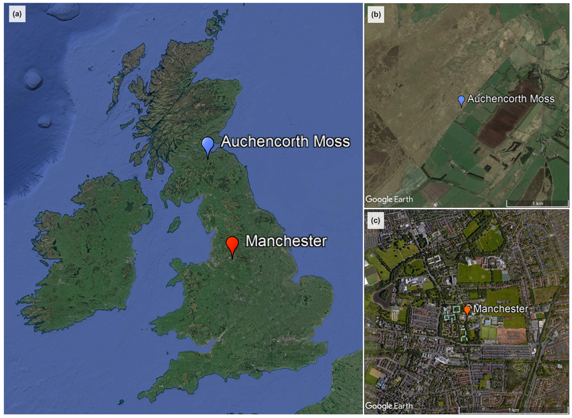
Measurements of j(NO2) were made at two locations in the UK (Figure 1): the rural background site at Auchencorth Moss ~18 km SSW of Edinburgh (55°47′ N, 3°14′ W, altitude 260 m) and the Manchester urban background air quality site located on the University of Manchester’s Fallowfield campus (53°26′ N, 2°12′ W, altitude 43 m).
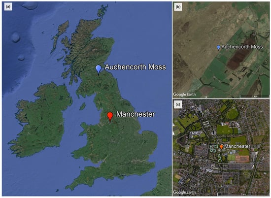
Figure 1.
(a) The locations in the UK of the Auchencorth Moss rural supersite and Manchester urban background supersite; (b,c) respectively show satellite images of the area surrounding each measurement site to ~1 km in all directions. Satellite imagery from Google Earth (2021).
Auchencorth Moss is a low-lying peatland, with an extensive fetch of open moorland in most directions (Figure 1b). It operates as a Level II/III EMEP ‘supersite’ representative of the northern UK background atmosphere [18] and hosts an extensive array of instrumentation to measure trace gas and aerosol concentrations [19] and meteorological variables [20].
A j(NO2) 4π filter radiometer (Metcon, Meteorologie Consult GmbH, Germany) is mounted on a mast ~3 m above ground level. Measurements are recorded at 1-s resolution, and two years of data are analysed here (1 January 2019–31 December 2020), excluding the period 5–26 June 2019 when the instrument was removed for calibration (described below). The position of the filter radiometer was carefully considered to minimise potential sources of local interference. It is situated at the outskirts of the site, away from all other physical features at the site (e.g., cabins, trees, other instruments), and its supporting mast has a matte black coating to reduce any reflection that would not otherwise occur. The ground beneath the instrument is largely long grasses, where features that could increase surface albedo (e.g., snow) are evenly distributed. The closest change in these features (~5 m behind the supporting mast) is a wooden slatted path covered in black non-slip mats. This could contribute some uncertainty to upwelling measurements, but as it is often obscured by vegetation is expected to be negligible.
The 4π sr filter radiometer provides a 360° field-of-view of the surrounding environment, by utilising two identical optical inlets facing in opposite directions (downwelling, ↓, facing zenith; and upwelling ↑, facing nadir). The inlet optic of each dome is designed to have a near-uniform angular response through use of a quartz diffusor [21], and is surrounded by a light shield to provide an ‘artificial horizon’, restricting the field-of-view for each dome to one hemisphere [12]. This allows total measured actinic flux, and therefore j(NO2), to be separated into its down- and upwelling components. Transmitted light is guided through a set of optical filters (2-mm UG3, 1-mm UG5, Schott GmbH) for the wavelengths of interest (310–420 nm) prior to their detection by a Hamamatsu photodiode, which proportionally converts incident radiation into an output voltage.
The filter radiometer was calibrated in Manchester against a Bentham DTM300 scanning spectroradiometer [2,22]. A mid-summer period of 13–25 June 2019 was selected to provide calibration over the maximum possible range of ambient incident radiation for the UK, between SZAs of 30–90°. The direction of the filter radiometer was turned 180° mid-way in order to calibrate each dome separately. Overall uncertainty in the spectroradiometer was ±5%, the sum in quadrature of uncertainties in instrumental parameters (including cosine and actinic head responses), measured wavelength and general setup. Values of j(NO2) were calculated from the actinic flux spectra collected using (NO2) from Mérienne et al. [23] and ϕ(NO2) from Troe [24].
Broadband measurements made by the filter radiometer (1 s) during each spectroradiometer scan (actinic flux measured in each narrow λ band (~0.8 nm) sequentially; 3 min total) were averaged to obtain a calibration comparison point. Large standard deviations associated with these mean values were used to remove calibration points where actinic flux was highly variable during a single scan (e.g., rapidly changing cloud cover), which would result in inconsistent conditions between λ intervals and yield an unrepresentative comparison to the filter radiometer. This range was primarily within ±5% of the mean calculated. The limits of detection (LOD; 3 of background signal) for the down- and upwelling domes were 9.40 × 10⁻⁶ s−1 and 1.15 × 10⁻⁵ s−1, respectively. Background signals were determined from averaged measurements made after sunset and before sunrise (SZA ≥ 96°) and removed prior to data analysis.
On a few occasions of peak solar irradiance (noon in summer), the maximum detector voltage of 9.6 V was reached. Instances of signals >9.5 V were therefore excluded. These comprise <1% of the raw data. An hourly average was only calculated if the 1 s data remaining within that hour met or exceeded 75% data capture. As a consequence, maximum j(NO2) presented in this study is an underestimate, estimated as 7–22% based on extrapolation of the calibrated relationship to the spectroradiometer. The upper limit in this range is for solar noon on a clear day around the summer solstice.
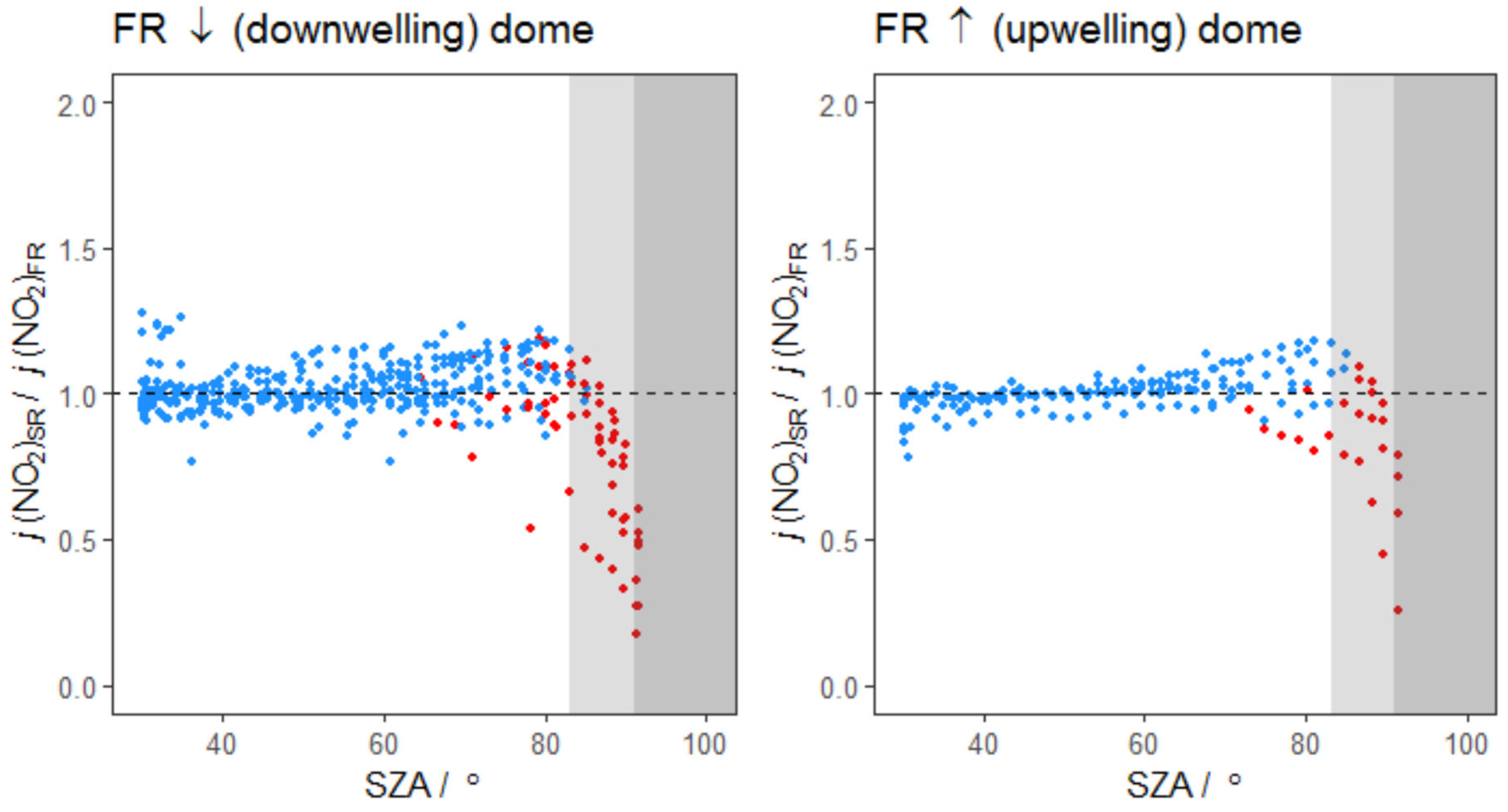
Ratio plots of j(NO2) measured by the spectroradiometer and each dome of the filter radiometer are presented as a function of SZA in Figure 2. Deviations from unity are observed predominantly at higher SZA, particularly during the ‘golden hour’, a colloquial term defined here as the sun being within 5° of the horizon. During this time measured values of j(NO2) are close to the LOD, and deviations in this ratio are larger. Using the same criteria as Bohn et al. [25], in their intercomparison of filter- and spectroradiometers, these low-light conditions are highlighted in Figure 2 via j(NO2) being <5% the observed maximum. These instances correspond with measurements at SZA > 85°.
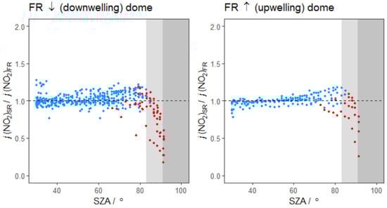
Figure 2.
Ratios of spectroradiometer to filter radiometer photolysis frequencies measured during the co-location calibration period as a function of SZA. Black dashed lines show the 1:1 ratio. Red points indicate values less than 5% of the maximum value for j(NO2) observed during the calibration. The light shading indicates SZA during the ‘golden hour’, defined here as 5° above the horizon, while the dark shading shows sunrise/sunset SZA of ≥90°.
The deviation from unity and the larger spread of data at the lower values of SZA (<80°) shown in Figure 2 can be attributed to synchronisation issues between the two measurement methods when conditions are not consistent. This includes periods of intermittent cloud cover resulting in shading or enhancement in solar radiation during a single spectroradiometer scan [26]. The extreme occurrences of this are removed via use of the standard deviation of averaged filter radiometer measurements described above, but some minor occurrences remain. Consequently, the spread of data is generally larger for the downwelling dome because there were more overcast conditions during its calibration than for the upwelling dome.
Overall, the uncertainty of the filter radiometer measurements were calculated as a combination of instrumental error [27], error from the calibration to this spectroradiometer, and errors due to external factors (e.g., temperature stability of the instrument). For six of the same filter radiometers, Shetter et al. [28] quote overall error as 9.6–11%, the range dependent on whether conditions were clear or cloudy. To provide a conservative estimate of error for both domes of the filter radiometer used here, the upper bound (11%; cloudy conditions) was combined with the calibration error of each dome. This yields an overall error for both the down- and upwelling domes of 13% for SZAs between 30 and 85°. For SZAs > 85°, the error increases to 32% and 25%, respectively.
As with the Auchencorth Moss site, the Manchester air quality supersite also incorporates a large suite of trace gas, aerosol and meteorological instruments, but is located to measure these quantities in the background air of a large UK city (Figure 1c). The actinic flux used to calculate the downwelling j(NO2) at this site is measured with an Ocean Optics spectrometer (FLAME-S-UV-VIS-ES) coupled to a 2π actinic flux optical inlet. The instrument was calibrated using an Optronic Laboratories FEL-C Irradiance Standard lamp performed in compliance with National Institute of Standards & Technology practices recommended in NIST Handbook 150-2E, Technical Guide for Optical Radiation Measurements [29]. The optical inlet is attached to black painted railings on top of the site hut, ~7.2 m above an asphalt car park. The nearest obstruction is some deciduous trees south of the site, reaching up to ~1.5 m above the height of the optical inlet, ~5 m away. This is anticipated to result in brief and intermittent shielding of radiation at SZA ≥ 73°. Measurements are recorded with a 1-min integration time and data for the period 6 September 2019 to 31 May 2020 are used here. The LOD for j(NO2), defined as 3 of the background signal measured when SZA was ≥96°, is 1.92 × 10⁻⁶ s−1.
2.2. Modelled Values of j(NO2)
Hourly model estimates for j(NO2) were calculated using the Tropospheric Ultraviolet and Visible radiation model (TUV v5.3) [8,30], used here to provide an example of modelled j(NO2) from one of the most widely used radiation models [31,32,33,34,35,36,37]. The model was set up to match the location and height of the radiometer at each site, and for cloud-free conditions, as an example of typical model estimations of j(NO2). A daily average ozone column for the model was obtained from the OMI satellite [38]. Days with missing O3 column measurements were filled with those from the following day. Air temperature was as measured at each site. Default TUV model values for surface albedo (0.1) and aerosol optical depth (AOD) at 550 nm [39] were used. The surface albedos of grass (Auchencorth Moss) and asphalt (Manchester) are similar to the default value. Variation in AOD between sites is assumed to be small and therefore have minor impact on modelled j(NO2). A value of 0.99 was set for the aerosol single-scattering albedo (SSA). Actual SSA is expected to be >0.8 [40], which in this model yields a maximum potential uncertainty in j(NO2)↓ of <12%. The NO2 column was assumed to be zero. Although NO2 column is actually anticipated to be in the range (6–15) × 1015 molecules cm−2 (approx. 0.25–0.5 DU) [41], inclusion of even the upper limit yields a maximum change in j(NO2)↓ of <2%. Other TUV model options remained at their default settings.
Since the radiometers at both sites are zenith-pointing, the TUV model domain replicates this 2π sr field-of-view by including only direct light and downward propagating diffuse radiation. However, as the Auchencorth Moss filter radiometer has a 4π sr field-of-view and includes a separate measurement of upwelling radiation, TUV was run a second time for Auchencorth Moss including upward propagating diffuse radiation. These model values are referred to as j(NO2)-down and j(NO2)-total, respectively.
2.3. Measurement-Driven Adjustment Factor
A measurement-driven adjustment factor (MDAF) for each hour at each site was derived as follows.
Two sets of MDAF values were calculated for Auchencorth Moss: one using the total signal measured by both domes of the filter radiometer, and the j(NO2)-total model results; and one using only the downwelling dome measurements, and the j(NO2)-down TUV output. MDAF values were excluded for SZA > 90°, i.e., between sunset and sunrise.
The quantum yield for NO2 photodissociation used by the TUV model is the same as that used in the calibration of the Auchencorth filter radiometer and Manchester spectroradiometer calculations [24], but the absorption cross-sections differ (value from Vandaele et al. [42] for the TUV model and from Mérienne et al. [23] for the filter radiometer calibration and spectroradiometer calculations). These differ by only 2–3% at ambient temperature [43].
3. Results and Discussion
3.1. The Need for Local Adjustments to j(NO2)
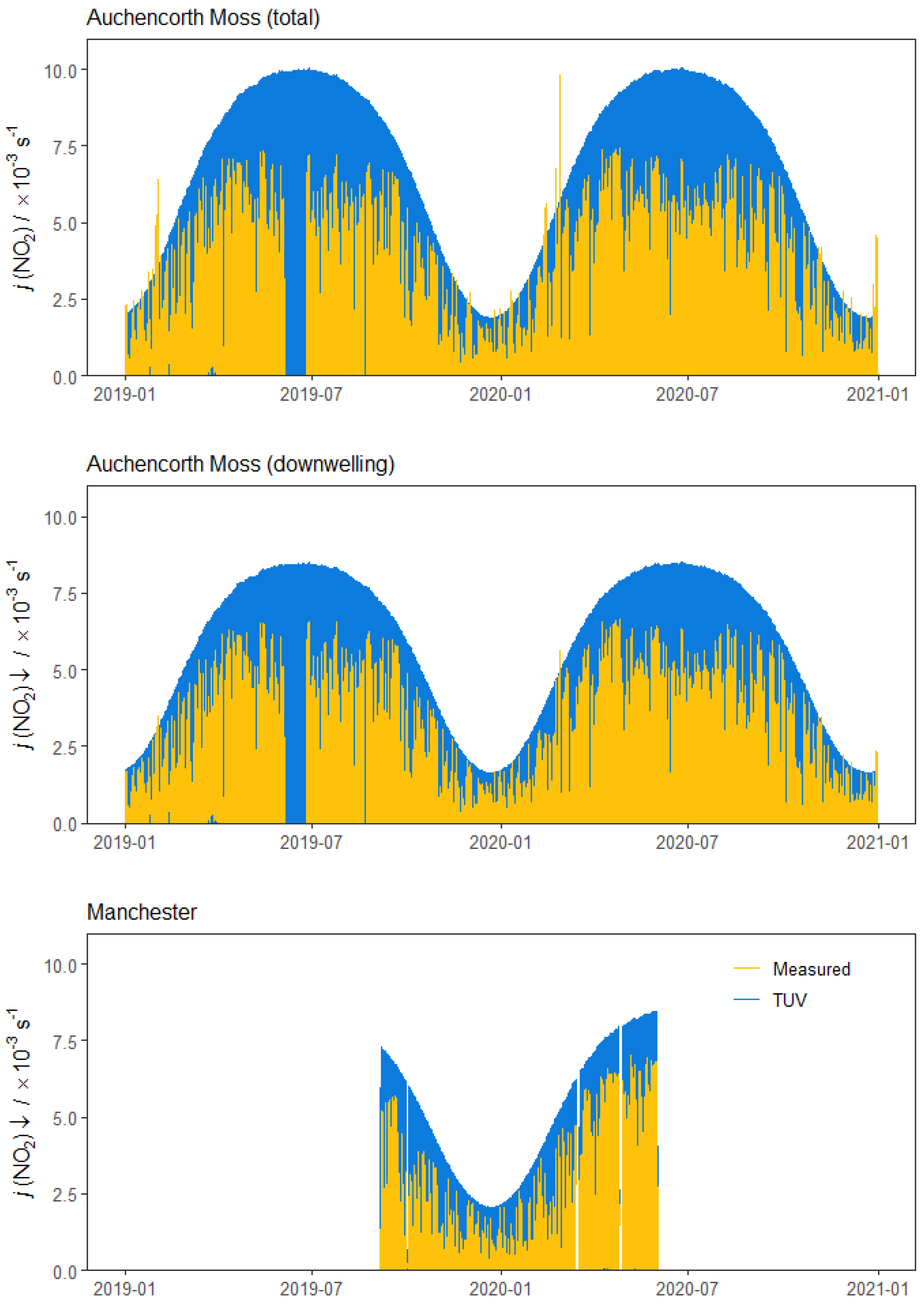
Measurements of j(NO2) exhibit the expected seasonal variation (Figure 3), with the smallest solar noon values observed in the winter (approximately 2.5 × 10⁻³ s−1; December to February), increasing through the spring (March to May) to a solar noon maximum of approximately 8 × 10⁻³ s−1 in the summer (June to August). (The large peaks in Auchencorth total j(NO2) measurements evident in winter are due to a large contribution of upwelling radiation, discussed in Section 3.2).

Figure 3.
Time series of hourly measured (yellow) and modelled (blue) j(NO2) at Auchencorth Moss and Manchester. Auchencorth data are presented for total (↓ + ↑) and downwelling-only j(NO2) (↓). The missing data in June 2019 are when the filter radiometer was removed for calibration.
Sites also demonstrate broadly similar temporal variation in j(NO2) measurements associated with synoptic-scale meteorological time resolution; for example, largest and smallest j(NO2) measurements are respectively associated with synoptic-scale high pressure and overcast conditions across the UK. However, at higher time resolution appropriate to air-quality photochemistry, the variation in local conditions at each site causes differences in measured j(NO2) values at the same time and on the same day: the hourly j(NO2) MDAF values derived for each site are shown in Figure 4, both as time series and as scatter plots with respect to SZA, whilst Figure 5 is a scatter plot of the hourly MDAF values at the two sites. The absence of correlation in Figure 5 demonstrates with contemporaneous data the extent to which local meteorology (e.g., cloud cover and aerosol profile) drives hourly variation in discrepancy between observed and modelled j(NO2) values and consequently that j(NO2) cannot be spatially extrapolated even over distances of a few 100 km.
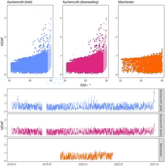
Figure 4.
Hourly derived measurement driven adjustment factors (MDAF) for j(NO2) at Auchencorth Moss (blue: total; pink: downwelling) and Manchester (orange). Top: MDAF values as a function of SZA. Bottom: time series of all hourly MDAF values. Auchencorth Moss filter radiometer measurements of higher uncertainty (>85°) have been filtered out of the time series, but are presented on the scatter plots in a lighter colour.
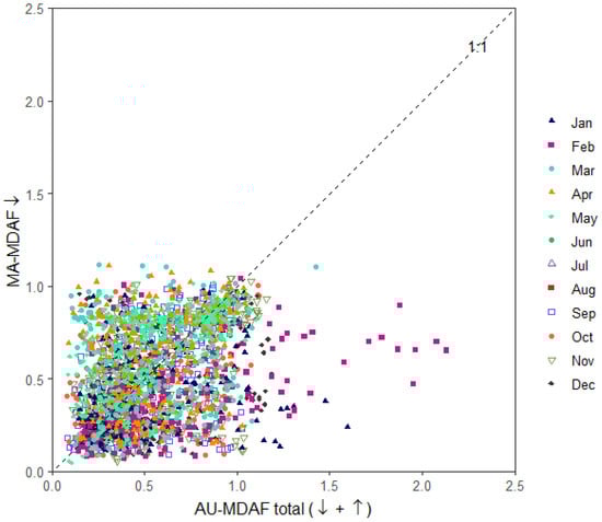
Figure 5.
Comparison of synchronous hourly Auchencorth Moss and Manchester MDAF values. Auchencorth data are for total j(NO2) (↓ + ↑). Colour and shape of points indicates month of measurement.
The scatter plots in Figure 4 also show that even when observed values are at their highest at both sites (reflecting clear-sky conditions at higher SZAs), the observed values are less than the TUV cloud-free estimates; i.e., the MDAF values are below unity, causing the corresponding model estimates to be scaled down. (Figure 3 illustrates the same feature.) The largest values of MDAF in Figure 4 decrease slightly with decreasing SZA in a generally linear trend, being lower than unity at SZA < 68° at Auchencorth Moss and <74° at Manchester. More scatter is observed in MDAF derivations at larger SZAs at Auchencorth Moss, caused by the measurement uncertainties discussed previously.
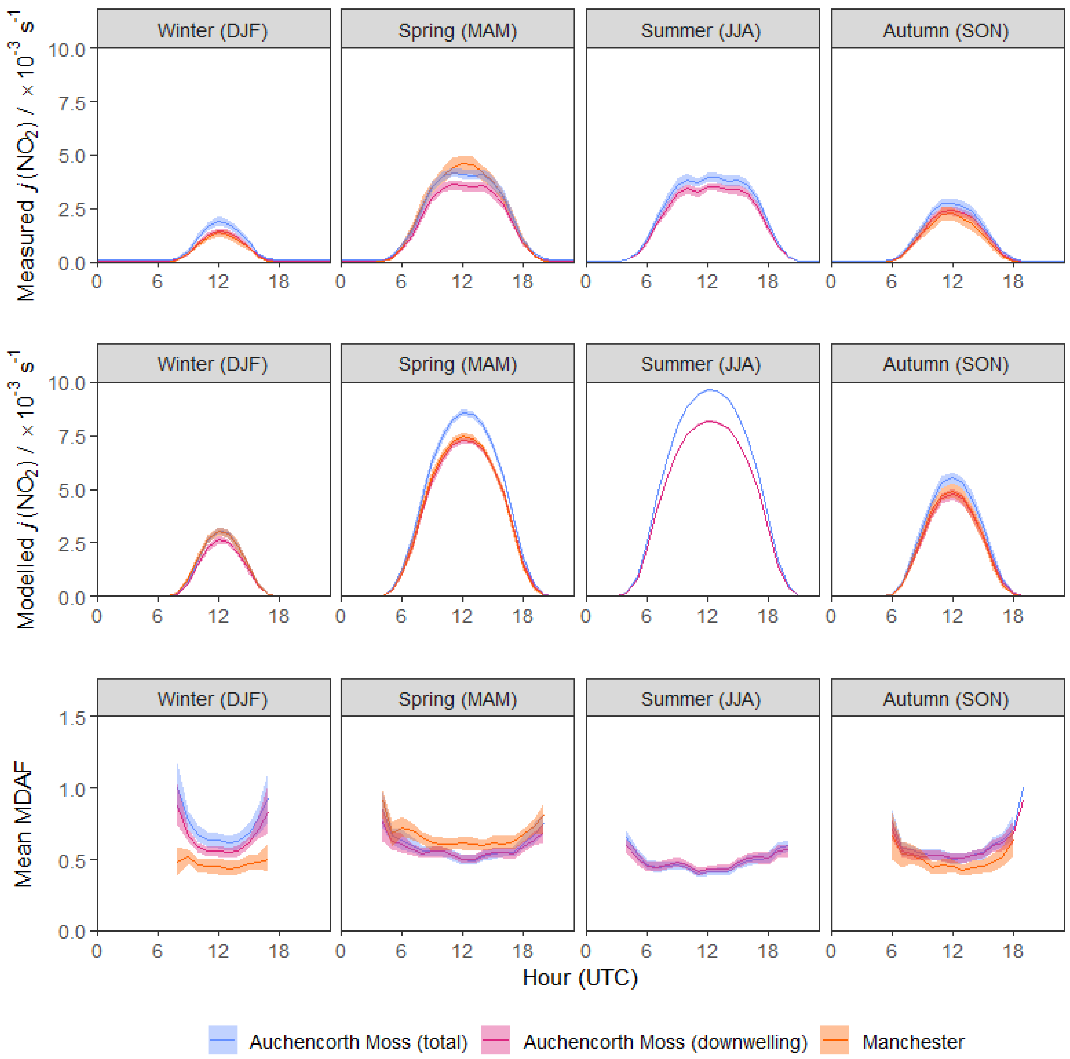
The magnitude of the influence of local meteorology is illustrated by the fact that the annual mean total and downwelling j(NO2) measured at Auchencorth Moss are respectively 44% and 45% lower than the annual mean cloud-free modelled j(NO2). The influence of local conditions not captured in the model estimates is further illustrated in Figure 6 which shows the seasonal mean diurnal profiles of measured and modelled j(NO2), and corresponding MDAF values, at the Auchencorth Moss and Manchester sites. In terms of modelled j(NO2), the expected inverse relationship with site latitude can be seen in Figure 6 since contemporaneous measurements have larger SZA at higher latitudes and scattering and absorption of solar radiation varies as ≈1/cos(SZA). This effect on modelled j(NO2) is relatively greater in autumn/winter when SZAs are larger. The j(NO2)↓ in autumn and winter at Manchester (53.4° N) is ~17–28% greater than at Auchencorth Moss (55.8° N).
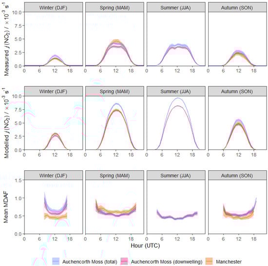
Figure 6.
Seasonal mean diurnal profiles of measured j(NO2), modelled j(NO2) and MDAF values at the Auchencorth Moss and Manchester sites. The shaded areas are the 95% confidence intervals of hourly data. There is no summer season data for Manchester.
Whilst the seasonal average MDAF values are broadly similar, there are small discrepancies between the two sites (Figure 6). At Manchester, the largest average reductions in modelled j(NO2) (shown by the smallest MDAF values in Figure 6) are in autumn and winter (51% and 53% reductions in j(NO2), respectively). These are seasons in which local meteorological conditions are characteristically more overcast. In spring, when the weather is typically clearer, the reduction in modelled j(NO2) is smaller (36%) and corresponding MDAF values are larger. In contrast, the winter mean MDAF values at Auchencorth Moss are smaller than at Manchester, with a mean winter reduction in measured j(NO2) compared with modelled j(NO2) of 31%. Figure 6 shows that this difference in winter mean MDAF values is contributed by the larger range in MDAF values at Auchencorth Moss, in particular the much larger MDAF values at larger SZA (sunrise and sunset). If only periods of higher solar intensity (with more direct light at larger SZAs) are considered at Auchencorth, the wintertime reduction in modelled j(NO2) at Auchencorth Moss is 45%, and similar to Manchester. This difference in winter averaged MDAF is attributed to interference from beyond the 2π sr view of the inlet optic being more prevalent at Auchencorth Moss, due to differences in the radiometer position at each site. The radiometer is fixed to a mast approximately 3 m above ground level (a.g.l.), while the Manchester spectroradiometer is attached to a cabin roof 7.2 m a.g.l. During periods of increased surface albedo, more diffuse upwelling radiation is collected by the downwelling dome of the radiometer than by the Manchester spectroradiometer, as it is closer to ground level. These occasions also occurred more frequently at Auchencorth Moss.
The key observation from Figure 6, however, is that at both sites local conditions give rise to measured j(NO2) values substantially lower than modelled. Figure 5 has shown that local conditions mean there is no contemporaneous correlation between the hourly measured MDAF values. Hence MDAF values derived at one site cannot readily be applied at another site.
3.2. 2π vs. 4π Filter Radiometer Values of MDAFs
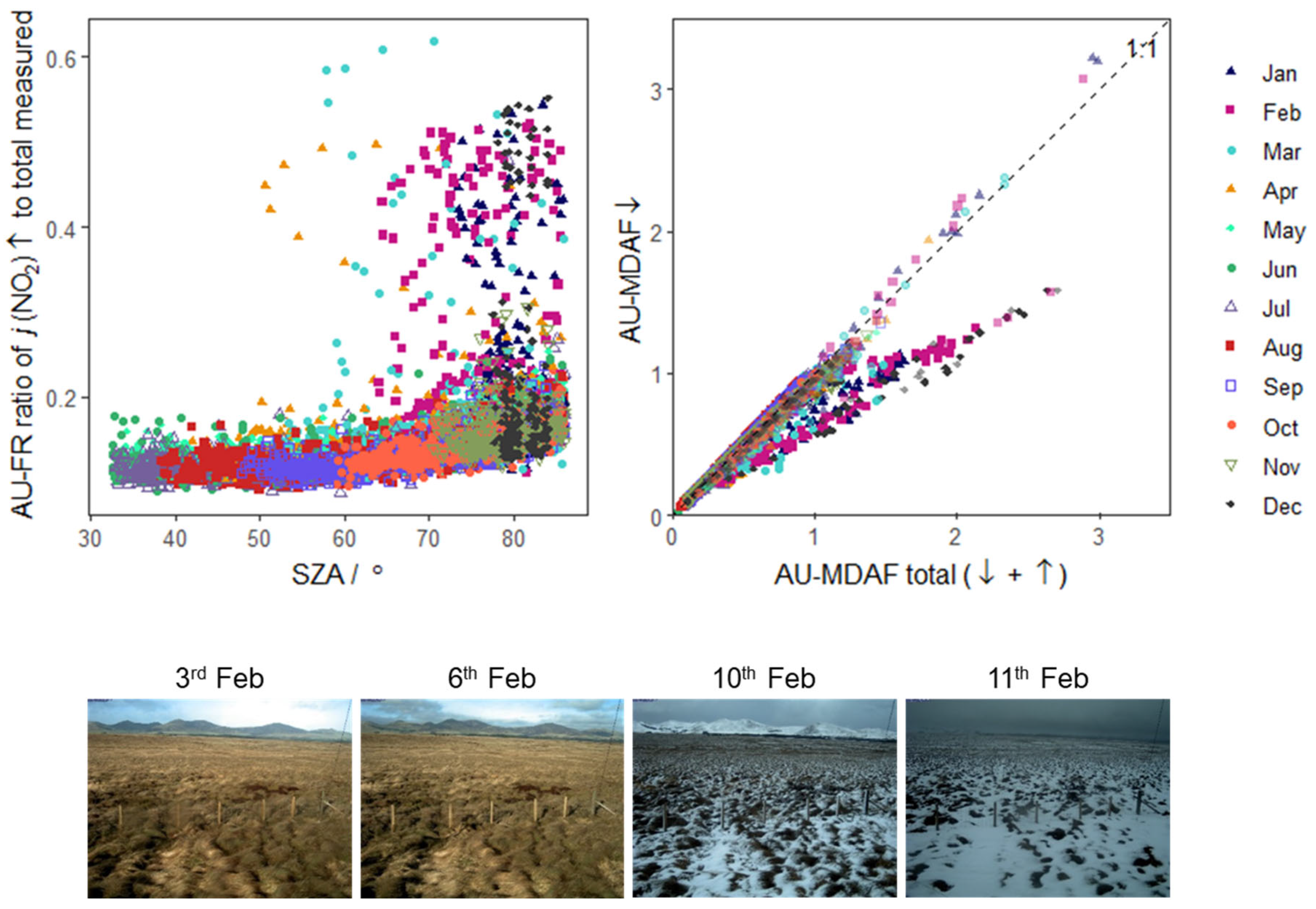
Measurements from the 4π filter radiometer at Auchencorth Moss can be separated into down- and upwelling components. The sensitivity of each dome reduces close to the horizon, but the total signal (sum of ↓ and ↑) is partially compensated by interference from the opposite facing dome resulting in a maximum overestimation of their actinic flux of 4% [44]. Both downwelling and total directions are visualised in Figure 7. The first panel shows the ratio of hourly mean upwelling j(NO2) measurements to the total, as a function of SZA; the second presents a direct comparison of the hourly MDAF values derived for both downwelling and total j(NO2). When considering diffuse direction from both zenith and nadir-facing directions, the TUV model consistently estimated j(NO2) values that were 15–17% larger than the 2π counterpart year-round, indicating that the seasonal difference in the Auchencorth Moss MDAF values are driven by measured j(NO2).

Figure 7.
(Left): ratios of hourly mean measured j(NO2) upwelling (↑) to total (↓ + ↑) as a function of SZA at Auchencorth Moss. (Right): scatterplot of hourly mean MDAF values derived using only downwelling j(NO2) against values derived using total j(NO2) (↓ + ↑). (Below): example photos of the site, taken by an automatic Phenocam (EuroPhen) at 12:00 UTC, for 3 and 6 February with no snow, whose hourly data lie on the 1:1 line in the right panel, and on 10, 13 February with snow, whose hourly data lie on the relationship below the 1:1 line.
The majority of j(NO2) to total j(NO2) ratios in Figure 7 are near-independent of SZA between 32° (minimum observed) and ~60°, but show a curved increase with SZA > 60°. This is expected, as at larger SZA there is increased partitioning of diffuse to direct radiation in the total. Compared to the middle of the day, less direct radiation is collected by the downwelling dome, while more diffuse radiation reaches the upwelling dome. This results in the contribution of the upwelling dome to total j(NO2) increasing to around half. Points above the main trend in the data represent irregular environmental changes that drive increased measurement of upwelling j(NO2), such as changes in surface albedo increasing the daytime contribution of upwelling radiation compared to the rest of the year. These occurrences were predominantly in January-March of both years, a short period at the end of December 2020, and a single day in April 2019.
For most of the year, derived Auchencorth Moss MDAF values for total and downwelling-only j(NO2) agree very well, lying close to the 1:1 line (Figure 7). However, there is a second well-correlated trend where the downwelling derived MDAF is approximately 60% of the total-radiation-derived MDAF, which corresponds with the identified days of increased upwelling radiation. This group of data have a slightly wider spread, due to larger variations in surface albedo caused by snow on the ground, as revealed in automated pictures of the site (Figure 7). In the TUV model, the surface albedo was left constant at 0.1; however, where snow is present, albedo is likely to be nearer to unity (0.8–0.9) [31,45]. On the days illustrated, the contribution of measured j(NO2)↑ to total j(NO2) rises to 48%. The increased contribution of upwelling j(NO2) translates to a 36% increase in the total MDAF compared to the MDAF derived for downwelling-only measurements. This demonstrates the importance of considering upwelling radiation on derived MDAF values in certain circumstances, which can have significant implications for adjustment of modelled values of j(NO2).
4. Conclusions and Implications
Local atmospheric chemistry and air quality modelling, such as is used to assess public health and the effectiveness of implemented mitigation measures, often includes highly parameterised photochemistry; and whilst modelled gas and aerosol concentrations are frequently validated against measurements, the same is rarely undertaken for photolytic fluxes, despite their importance also to model simulations. This is usually due to a lack of measured photolytic data outside of specific campaigns. The study reported here has demonstrated the use of local radiometer measurements for capturing via a measurement-driven adjustment factor (MDAF) the variability at high temporal resolution which is needed to adjust clear-sky or cloud-free model estimates. Measurements at Auchencorth Moss and Manchester in the UK showed that TUV (v5.3) model estimates of j(NO2)↓ in cloud-free conditions (as an example of modelled j-values) were, on average, approximately 45% larger than measured j(NO2)↓, which would lead to bias in models if there was no adjustment to account for local conditions.
At Auchencorth Moss, MDAF values considering 4π and 2π sr fields of view have good agreement (<6% difference, on average) for most conditions. However, conditions of particularly high surface albedo (such as snow cover) increase the upwelling component of the local diffuse radiation. Consequently, under these conditions the MDAF based on total radiation (considering both j(NO2)↓ and j(NO2)↑) is around 40% larger than the MDAF derived when only downwelling j(NO2)↓ is considered.
The study has demonstrated, firstly, the magnitude of potential impact of local conditions—principally cloud cover, but also changes in surface albedo—on assumed j-values. Secondly, that whilst annual average MDAF values are similar at Auchencorth Moss and Manchester, at hourly time resolution differences in local conditions mean there is no contemporaneous correlation between j(NO2) values. Hence MDAF values derived at one site cannot readily be applied at another site.
Although the TUV modelling conducted for this study was limited by some assumptions in input parameters (e.g., SSA and O3 column), the modelled j(NO2) values in this study provide a typical estimate of cloud-free modelled j(NO2), and therefore a useful baseline to demonstrate the need for MDAF application at different sites. (The study was not an examination of absolute modelled j(NO2) per se.)
Radiometer j(NO2) measurements such as those analysed here are now starting to be made in a long-term capacity in the UK and in continental Europe (at least 4 ACTRIS sites; personal communication). The standardisation and archiving of these long-term multi-site measurements will be of immense support to atmospheric chemistry modelling. First, the measurements can be used directly within models to constrain j(NO2). Secondly, they can be used to derive a MDAF metric to scale modelled j-values of other photodissociation reactions, as has been done in previous studies e.g., [13,14,15,17]. This use of MDAF expands the application of j(NO2) measurements to a number of important radical producing photodissociation reactions, such as the HOx sources of HONO and HCHO, and the Cl atom source of ClNO2. An analysis of applying an MDAF value derived from a reference species such as j(NO2) (and j(O1D) to other modelled photolysis rate constants is detailed in Walker et al. [46].
Measurements of j(NO2) would be particularly advantageous in urban environments. Such measurements would be hyper-specific to individual locations, as even small differences in location could provide very different light levels due to the high variability in the local environment. A wide array of nearby materials may provide different surface albedos that alter the measured actinic flux, and the lack of uniformity in local features (e.g., buildings) can result in unique temporal patterns of shadows at each site. This emphasises the need for international collaboration in the routine deployment of long-term radiometer measurements alongside compositional measurements to support atmospheric chemistry modelling.
Author Contributions
Conceptualization and methodology, H.L.W., M.R.H., C.F.B. and M.M.T.; formal analysis and investigation, H.L.W.; resources, S.R.L., I.S. M.R.J., R.K. and N.M.; writing—original draft preparation, H.L.W.; writing—review and editing, H.L.W., M.R.H., M.M.T. and C.F.B. All authors have read and agreed to the published version of the manuscript.
Funding
H.L.W. acknowledges studentship funding from the UK Centre for Ecology & Hydrology (CEH) co-funding of Environment Agency Contract grant NEC05967 and the University of Edinburgh School of Chemistry. The operation of the filter radiometer at Auchencorth Moss was supported by the UK Natural Environment Research Council grant NE/R016429/1 as part of the UK-SCAPE programme delivering National Capability.
Data Availability Statement
The measured and simulated hourly j(NO2) values are available on request from the corresponding author.
Acknowledgments
The authors acknowledge permission from Carole Helfter (UKCEH) for the Phenocam images of Auchencorth Moss in Figure 7, and the UK Department for Environment, Food and Rural Affairs (Defra) and the Devolved Administrations for maintaining instrument operations (ECM48524).
Conflicts of Interest
The authors declare no conflict of interest.
References
- Chen, C.-H.; Chen, T.-F.; Huang, S.-P.; Chang, K.-H. Comparison of the RADM2 and RACM chemical mechanisms in O3 simulations: Effect of the photolysis rate constant. Sci. Rep. 2021, 11, 5024. [Google Scholar] [CrossRef] [PubMed]
- Thiel, S.; Ammannato, L.; Bais, A.; Bandy, B.; Blumthaler, M.; Bohn, B.; Engelsen, O.; Gobbi, G.P.; Gröbner, J.; Jäkel, E.; et al. Influence of clouds on the spectral actinic flux density in the lower troposphere (INSPECTRO): Overview of the field campaigns. Atmos. Chem. Phys. 2008, 8, 1789–1812. [Google Scholar] [CrossRef] [Green Version]
- Wang, W.; Li, X.; Shao, M.; Hu, M.; Zeng, L.; Wu, Y.; Tan, T. The impact of aerosols on photolysis frequencies and ozone production in Beijing during the 4-year period 2012–2015. Atmos. Chem. Phys. 2019, 19, 9413–9429. [Google Scholar] [CrossRef] [Green Version]
- Zhao, S.; Hu, B.; Liu, H.; Du, C.; Xia, X.; Wang, Y. The influence of aerosols on the NO2 photolysis rate in a suburban site in North China. Sci. Total Environ. 2021, 767, 144788. [Google Scholar] [CrossRef]
- Azzi, M.; Johnson, G.M.; Cope, M.E. An introduction to the generic reaction set photochemical smog mechanism. Proc. Elev. Int. Conf. Clean Air Soc. Aust. N. Z. 1992, 2, 451–462. Available online: https://publications.csiro.au/rpr/pub?list=BRO&pid=procite:fd8053cf-f783-48f8-b218-e01de4961266 (accessed on 1 June 2022).
- Jenkin, M.E.; Saunders, S.M.; Pilling, M.J. The tropospheric degradation of volatile organic compounds: A protocol for mechanism development. Atmos. Environ. 1997, 31, 81–104. [Google Scholar] [CrossRef]
- Saunders, S.M.; Jenkin, M.E.; Derwent, R.G.; Pilling, M.J. Protocol for the development of the Master Chemical Mechanism, MCM v3 (Part A): Tropospheric degradation of non-aromatic volatile organic compounds. Atmos. Chem. Phys. 2003, 3, 161–180. [Google Scholar] [CrossRef] [Green Version]
- NCAR. National Centre for Atmospheric Research (NCAR) Tropospheric Ultraviolet and Visible (TUV) Radiation Model v5.3. 2019. Available online: https://www2.acom.ucar.edu/modeling/tropospheric-ultraviolet-and-visible-tuv-radiation-model (accessed on 1 June 2022).
- Neu, J.L.; Prather, M.J.; Penner, J.E. Global atmospheric chemistry: Integrating over fractional cloud cover. J. Geophys. Res. 2007, 112, D11306. [Google Scholar] [CrossRef] [Green Version]
- Monks, P.S.; Granier, C.; Fuzzi, S.; Stohl, A.; Williams, M.L.; Akimoto, H.; Amann, M.; Baklanov, A.; Baltensperger, U.; Bey, I.; et al. Atmospheric composition change—Global and regional air quality. Atmos. Environ. 2009, 43, 5268–5350. [Google Scholar] [CrossRef] [Green Version]
- Junkermann, W.; Platt, U.; Volz-Thomas, A. A photoelectric detector for the measurement of photolysis frequencies of ozone and other atmospheric molecules. J. Atmos. Chem. 1989, 8, 203–227. [Google Scholar] [CrossRef]
- Volz-Thomas, A.; Lerner, A.; Pätz, H.-W.; Schultz, M.; McKenna, D.S.; Schmitt, R.; Madronich, S.; Röth, E.P. Airborne measurements of the photolysis frequency of NO2. J. Geophys. Res. 1996, 101, 18613–18627. [Google Scholar] [CrossRef]
- Elshorbany, Y.F.; Kleffmann, J.; Hofzumahaus, A.; Kurtenbach, R.; Wiesen, P.; Brauers, T.; Bohn, B.; Dorn, H.-P.; Fuchs, H.; Holland, F.; et al. HOx budgets during HOxComp: A case study of HOx chemistry under NOx-limited conditions. J. Geophys. Res. 2012, 117, D03307. [Google Scholar] [CrossRef] [Green Version]
- Bannan, T.J.; Bacak, A.; Le Breton, M.; Flynn, M.; Ouyang, B.; McLeod, M.; Jones, R.; Malkin, T.L.; Whalley, L.K.; Heard, D.E.; et al. Ground and Airborne U.K. Measurements of Nitryl Chloride: An Investigation of the Role of Cl Atom Oxidation at Weybourne Atmospheric Observatory. J. Geophys. Res. 2017, 122, 11154–111165. [Google Scholar] [CrossRef]
- Xue, C.; Zhang, C.; Ye, C.; Liu, P.; Catoire, V.; Krysztofiak, G.; Chen, H.; Ren, Y.; Zhao, X.; Wang, J.; et al. HONO Budget and Its Role in Nitrate Formation in the Rural North China Plain. Environ. Sci. Technol. 2020, 54, 11048–11057. [Google Scholar] [CrossRef]
- Sommariva, R.; Cox, S.; Martin, C.; Borońska, K.; Young, J.; Jimack, P.K.; Pilling, M.J.; Matthaios, V.N.; Nelson, B.S.; Newland, M.J.; et al. AtChem (version 1), an open-source box model for the Master Chemical Mechanism. Geosci. Model Dev. 2020, 13, 169–183. [Google Scholar] [CrossRef] [Green Version]
- Sommariva, R.; Crilley, L.R.; Ball, S.M.; Cordell, R.L.; Hollis, L.D.J.; Bloss, W.J.; Monks, P.S. Enhanced wintertime oxidation of VOCs via sustained radical sources in the urban atmosphere. Environ. Pollut. 2021, 274, 116563. [Google Scholar] [CrossRef]
- Malley, C.S.; Braban, C.F.; Heal, M.R. The application of hierarchical cluster analysis and non-negative matrix factorization to European atmospheric monitoring site classification. Atmos. Res. 2014, 138, 30–40. [Google Scholar] [CrossRef] [Green Version]
- Twigg, M.M.; Di Marco, C.F.; Leeson, S.; van Dijk, N.; Jones, M.R.; Leith, I.D.; Morrison, E.; Coyle, M.; Proost, R.; Peeters, A.N.M.; et al. Water soluble aerosols and gases at a UK background site—Part 1: Controls of PM2.5 and PM10 aerosol composition. Atmos. Chem. Phys. 2015, 15, 8131–8145. [Google Scholar] [CrossRef] [Green Version]
- Coyle, M.; Cape, J.N.; Flechard, C.; Fowler, D.; Helfter, C.; Jones, M.; Kentisbeer, J.; Leeson, S.R.; Leith, I.D.; Mullinger, N.; et al. Meteorological measurements at Auchencorth Moss from 1995 to 2016. Geosci. Data J. 2019, 6, 16–29. [Google Scholar] [CrossRef]
- Bohn, B.; Kraus, A.; Müller, M.; Hofzumahaus, A. Measurement of atmospheric O3 → O(1D) photolysis frequencies using filterradiometry. J. Geophys. Res. 2004, 109, D10S90. [Google Scholar] [CrossRef] [Green Version]
- Webb, A.R.; Bais, A.F.; Blumthaler, M.; Gobbi, G.P.; Kylling, A.; Schmitt, R.; Thiel, S.; Barnaba, F.; Danielsen, T.; Junkermann, W.; et al. Measuring Spectral Actinic Flux and Irradiance: Experimental Results from the Actinic Flux Determination from Measurements of Irradiance (ADMIRA) Project. J. Atmos. Ocean. Technol. 2002, 19, 1049–1062. [Google Scholar] [CrossRef]
- Mérienne, M.F.; Jenouvrier, A.; Coquart, B. The NO2 absorption spectrum. I: Absorption cross-sections at ambient temperature in the 300–500 nm region. J. Atmos. Chem. 1995, 20, 281–297. [Google Scholar] [CrossRef]
- Troe, J. Are Primary Quantum Yields of NO2 Photolysis at λ ≤ 398 nm Smaller than Unity? Z. Phys. Chem. 2000, 214, 573. [Google Scholar] [CrossRef]
- Bohn, B.; Corlett, G.K.; Gillmann, M.; Sanghavi, S.; Stange, G.; Tensing, E.; Vrekoussis, M.; Bloss, W.J.; Clapp, L.J.; Kortner, M.; et al. Photolysis frequency measurement techniques: Results of a comparison within the ACCENT project. Atmos. Chem. Phys. 2008, 8, 5373–5391. [Google Scholar] [CrossRef] [Green Version]
- Schade, N.H.; Macke, A.; Sandmann, H.; Stick, C. Enhanced solar global irradiance during cloudy sky conditions. Meteorol. Z. 2007, 16, 295–303. [Google Scholar] [CrossRef]
- Larason, T.C.; Cromer, C.L. Sources of Error in UV Radiation Measurements. J. Res. Natl. Inst. Stand. Technol. 2001, 106, 649–656. [Google Scholar] [CrossRef]
- Shetter, R.E.; Junkermann, W.; Swartz, W.H.; Frost, G.J.; Crawford, J.H.; Lefer, B.L.; Barrick, J.D.; Hall, S.R.; Hofzumahaus, A.; Bais, A.; et al. Photolysis frequency of NO2: Measurement and modeling during the International Photolysis Frequency Measurement and Modeling Intercomparison (IPMMI). J. Geophys. Res. 2003, 108, 8544. [Google Scholar] [CrossRef] [Green Version]
- Faison, C.; Brickencamp, C. NIST HANDBOOK 150-2E National Voluntary Laboratory Accreditation Program Calibration Laboratories Technical Guide for Optical Radiation Measurements; National Institute of Standards and Technology: Gaithersburg, MD, USA, 2001. Available online: https://tsapps.nist.gov/publication/get_pdf.cfm?pub_id=905613 (accessed on 1 June 2022).
- Madronich, S. Photodissociation in the atmosphere: 1. Actinic flux and the effects of ground reflections and clouds. J. Geophys. Res. 1987, 92, 9740–9752. [Google Scholar] [CrossRef]
- Lee-Taylor, J.; Madronich, S. Calculation of actinic fluxes with a coupled atmosphere–snow radiative transfer model. J. Geophys. Res. 2002, 107, ACH 22-1–ACH 22-10. [Google Scholar] [CrossRef]
- Bais, A.F.; Madronich, S.; Crawford, J.; Hall, S.R.; Mayer, B.; van Weele, M.; Lenoble, J.; Calvert, J.G.; Cantrell, C.A.; Shetter, R.E.; et al. International Photolysis Frequency Measurement and Model Intercomparison (IPMMI): Spectral actinic solar flux measurements and modeling. J. Geophys. Res. 2003, 108, 8543. [Google Scholar] [CrossRef]
- Wilson, S.R. Characterisation of J(O1D) at Cape Grim 2000–2005. Atmos. Chem. Phys. 2015, 15, 7337–7349. [Google Scholar] [CrossRef] [Green Version]
- Bohn, B.; Heard, D.E.; Mihalopoulos, N.; Plass-Dülmer, C.; Schmitt, R.; Whalley, L.K. Characterisation and improvement of j(O1D) filter radiometers. Atmos. Meas. Tech. 2016, 9, 3455–3466. [Google Scholar] [CrossRef] [Green Version]
- Ghosh, D.; Sarkar, U. Analysis of the photochemical production of ozone using Tropospheric Ultraviolet-Visible (TUV) Radiation Model in an Asian megacity. Air Qual. Atmos. Health 2016, 9, 367–377. [Google Scholar] [CrossRef]
- Wang, J.; Zhang, X.; Guo, J.; Wang, Z.; Zhang, M. Observation of nitrous acid (HONO) in Beijing, China: Seasonal variation, nocturnal formation and daytime budget. Sci. Total Environ. 2017, 587–588, 350–359. [Google Scholar] [CrossRef]
- Xu, W.; Kuang, Y.; Zhao, C.; Tao, J.; Zhao, G.; Bian, Y.; Yang, W.; Yu, Y.; Shen, C.; Liang, L.; et al. NH3-promoted hydrolysis of NO2 induces explosive growth in HONO. Atmos. Chem. Phys. 2019, 19, 10557–10570. [Google Scholar] [CrossRef] [Green Version]
- NOAA. National Oceanic and Atmospheric Administration—Integrated Surface Database (NOAA-ISD). 2022. Available online: https://www.ncei.noaa.gov/products/land-based-station/integrated-surface-database (accessed on 1 June 2022).
- Elterman, L. UV, Visible, and IR Attenuation for Altitudes to 50 km; Air Force Cambridge Research Laboratories (AFCRL): Cambridge, MA, USA, 1968. [Google Scholar]
- Madronich, S. The Atmosphere and UV-B Radiation at Ground Level. In Environmental UV Photobiology; Young, A.R., Moan, J., Björn, L.O., Nultsch, W., Eds.; Springer: Boston, MA, USA, 1993. [Google Scholar]
- Pope, R.J.; Arnold, S.R.; Chipperfield, M.P.; Latter, B.G.; Siddans, R.; Kerridge, B.J. Widespread changes in UK air quality observed from space. Atmos. Sci. Lett. 2018, 19, e817. [Google Scholar] [CrossRef]
- Vandaele, A.C.; Hermans, C.; Simon, P.C.; Carleer, M.; Colin, R.; Fally, S.; Mérienne, M.F.; Jenouvrier, A.; Coquart, B. Measurements of the NO2 absorption cross-section from 42,000 cm−1 to 10,000 cm−1 (238–1000 nm) at 220 K and 294 K. J. Quant. Spectrosc. Radiat. Transf. 1998, 59, 171–184. [Google Scholar] [CrossRef] [Green Version]
- Burkholder, J.B.; Sander, S.P.; Abbatt, J.P.D.; Barker, J.R.; Cappa, C.; Crounse, J.D.; Dibble, T.S.; Huie, R.E.; Kolb, C.E.; Kurylo, M.J.; et al. Chemical Kinetics and Photochemical Data for Use in Atmospheric Studies; Evaluation Number 19; Jet Propulsion Laborary: Pasadena, CA, USA, 2020; Available online: https://hdl.handle.net/2014/49199 (accessed on 1 June 2022).
- Hofzumahaus, A.; Kraus, A.; Kylling, A.; Zerefos, C.S. Solar actinic radiation (280–420 nm) in the cloud-free troposphere between ground and 12 km altitude: Measurements and model results. J. Geophys. Res. 2002, 107, PAU 6-1–PAU 6-11. [Google Scholar] [CrossRef]
- Lin, W.; Zhu, T.; Song, Y.; Zou, H.; Tang, M.; Tang, X.; Hu, J. Photolysis of surface O3 and production potential of OH radicals in the atmosphere over the Tibetan Plateau. J. Geophys. Res. 2008, 113, D02309. [Google Scholar] [CrossRef]
- Walker, H.L.; Heal, M.R.; Braban, C.F.; Whalley, L.K.; Twigg, M.M. Investigating the application of local measurement-driven adjustment factors for modelled atmospheric photolysis rate coefficients. Environ. Sci. Atmos. 2022. submitted. [Google Scholar]


Publisher’s Note: MDPI stays neutral with regard to jurisdictional claims in published maps and institutional affiliations. |
© 2022 by the authors. Licensee MDPI, Basel, Switzerland. This article is an open access article distributed under the terms and conditions of the Creative Commons Attribution (CC BY) license (https://creativecommons.org/licenses/by/4.0/).