Abstract
This research examines the persistence of a pandemic in urban environments subjected to intensive densification processes, applying chaotic analysis tools to hourly time series constructed by relating accumulated patients with meteorological and pollutant variables (measured at ground level). To investigate this objective, seven communes of the metropolitan region of Santiago de Chile that present intensive urbanization processes that affect urban micrometeorology, favoring the concentration of pollutants, were considered. Quotients were constructed between the number of hourly patients with SARS-CoV-2 that accumulated in each commune over a period of two years and the hourly variables of urban micrometeorology (temperature, magnitude of wind speed, relative humidity) and pollutant concentration (tropospheric ozone, particulate material of 2.5 and 10 μm) constituting a new family of time series. Chaos theory was applied to these new time series, obtaining the chaotic parameters Lyapunov coefficient, correlation entropy, Lempel–Ziv complexity, Hurst coefficient and the fractal dimension in each measurement commune. The results showed that the accumulated patients (2020–2022), of the order of 400,000, belonged to the five communes (with a built area of approximately 300,000 m2 in recent years) that had the highest urban densification, which affected urban meteorology, favored the concentration of pollutants and made the SARS-CoV-2 pandemic more persistent. The “ideal” density of built housing should balance a pandemic and nullify its expansion.
1. Introduction
This research addresses the problem of the spread of a pandemic from the perspective of chaos theory [1,2,3] applied to hourly time series of meteorological and pollutant variables. From ratios between accumulated hourly patients and hourly measurements of meteorological variables and pollutants, new time series were constructed. Following studies that have applied this procedure [4], it follows that the first condition that the time series of meteorological variables and pollutants must satisfy is that they be nonlinear. These series were obtained from the SINCA—Air Quality National Information System—[5] dependent on the Chilean Ministry of the Environment (for Abbreviations). On each of these series, we calculated the chaotic parameters Lyapunov coefficients (λ), the correlation dimension (DC), the Kolmogorov entropy (SK), the Hurst coefficient (H) and the Lempel–Ziv complexity (LZ) [2], proving that all the time series were chaotic. The second condition arises from analyzing the relationship of each of the time series with the accumulated patients according to the communes under study [6]. Each of these new hourly series also has a set of chaotic parameters such as those indicated. Based on this information, the accumulated patients, the entropies, the Lempel–Ziv complexity, the loss of information, the fractal dimension were studied comparatively among the communes considered. The analysis explains the dispersion and sustainability of the pandemic by weighing the increase in high-rise buildings and urban densification with urban meteorology and the concentration of atmospheric pollutants. These results can be used to characterize the tropospheric environment of the commune with the spread of the pandemic and compare with official indicators of communes with more infections [6].
1.1. Pandemics Antecedents
Epidemic patterns have shown notable changes throughout this century. In childhood infectious diseases, such as measles, the main transitions are between regular and irregular cycles, possibly chaotic, and regionally synchronized with a geographical distribution without a defined pattern [1]. A recent study [7] analyzed the virus in aerosols, concluding that aerosols (less than 5 μm) containing SARS-CoV-2 (105.25 50% tissue culture infectious dose (TCID50 per mL)) or SARS-CoV-1 (106.75 7.00 TCID50 per mL), recorded threshold values similar to those observed in samples obtained from the upper and lower respiratory tract in humans. According to the article, SARS-CoV-2 remained viable in aerosols in the order of 3 h during the experiment, with a reduction in the infectious titer from 103.5 to 102.7 TCID50 per mL. This reduction was similar to that observed with SARS-CoV-1, from 104.3 to 103.5 TCID50 per mL. The percentage of tissue culture infectious dose assay is a traditional method used by virologists to determine viral titers in both stocks and samples.
According to experts from the group that promotes the theory of the transmission of the pandemic by air, a possible proof would be provided by what happened in a choir in the United States. One person infected 53 others, after a trial of two-and-a-half hours. There was no contact and social distance was respected. The only explanation would be that the virus spread through the air [8,9,10,11]. Other studies [12] have been carried out regarding the effect of meteorology on the spread of the pandemic and from an urban point of view [13] in other epidemics. The problem of the coronavirus in urban centers has been treated by various authors. In [14,15], several areas of action are characterized: transformations in the configuration of public spaces, transportation, urban connectivity and urban economies. The pandemic has also been studied according to a systemic approach [16,17,18,19], as a set of interrelated elements with a common goal. Shannon’s entropy formalism [20] can be projected to real data (number of confirmed cases versus time (days, weeks)). The purpose is to examine the characteristics of the pandemic under the assumption that human activity, even in pandemic times, can trigger subsequent waves. In [4], the chaotic study was applied to hourly time series, over a period of three months, showing that the meteorology and pollutants can favor the increase in accumulated patients from a coronavirus-type pandemic.
A total of seven communes of Santiago de Chile participated in this investigation with measurements from 03/30/20 to 04/18/22. For each commune, the following was studied: 1. hourly meteorology time series (temperature (T), relative humidity (HR), magnitude of the wind speed (WS)), 2. hourly pollutant time series (tropospheric ozone (O3), PM2.5 particulate matter, PM10 particulate matter), 3. the relationship between intensive urbanization with the change in surface roughness and, 4. how this set of variables can influence the number of accumulated patients. This allowed us to check if there was a relationship between urban meteorology, thermal islands, urban canyons, overcrowding and roughness, which limited heat dissipation and ventilation, favoring the spread of the virus. Specifically, if a virus enters the human body through the respiratory tract, then urban micrometeorology is closely connected to the change in surface roughness, favoring the sustainability and spread of contaminants, making the infection, cultivation and spread of the virus more effective.
1.2. Micrometeorology
This is the area of meteorology that deals with observations and processes on smaller scales of space and time [21], in the order of 1 km and measurement periods of one hour or less. These processes are limited to the lower part of the planetary boundary layer, known as the atmospheric boundary layer (ABL) [22]. Its foundations are determined by the exchange of energy, mass and gasses between the atmosphere and the base surface (water, soil, plants). The study of temperature and wind (turbulence) being affected by external factors, such as buildings [23], flora, population and relief, is of paramount relevance. International networks of flow control sites use micrometeorological techniques to understand the exchange of energy and mass between the biosphere and the atmosphere [22]. On the one hand, heat transfer through the boundary layer firstly occurs by molecular diffusion and then by turbulent diffusion [23]. In such environments, the flow structure in the roughness sublayer dictates the air flow and pollutant dispersion within and above urban canopies [20,24]. This sublayer consists of the lowest part of the atmospheric surface layer, from the ground to 2–5 times the average height of the canopy elements. Moreover, the roughness sublayer is where the turbulent exchange of momentum, heat and mass occurs [25,26]. On the other hand, turbulence enables the exchange of CO2 between plants and the atmosphere, whilst also aiding the distribution of pollen. Finally, buildings play a crucial role within micrometeorology, as they increase turbulence and thermal sensation in cities [21,23].
1.3. Urban Densification
Many cities in Chile have urban growth that is becoming unsustainable, especially in densely populated metropolitan areas. This study used public data [27,28] to analyze the urban density and the change in roughness of the selected places. From a housing approach, the comparative study is important. According to official data [27,28], the number of residential properties (N°) between the years (t) 2009–2020 grew exponentially:
By 2015, many of the buildings were 15 floors. In 2020, the majority were 30 floors. The supply of apartments (2020) increased by 77.3%. In the Metropolitan Region there were 50 homes per hectare in 1990; in 2020, there were around 5000 homes per hectare [27,28]. According to census data from 1970, the proportion of apartments in Chile was only 7% (116,748). Since then, that alternative has been widely more accepted by the Chilean people, so that in 2002, that percentage reached 12.6% (474,199, according to the 2002 census). In 2018, they represented 17.5% of a total of 1,138,062 homes (552,678 more than in 2002) [27]. In the following years, this verticalization process continued intensively through buildings made of concrete. The monitoring stations used in this study are located in areas that have gone through an intense process of high-rise building, that affect urban micrometeorology, making it more turbulent. For the crop canopy, the average in the metropolitan region in 2017 was 6.4 m2/inhabitant, while in 2021, it was 6.2 m2/inhabitant. The minimum value recommended by [29] is 9 to 11 m2/inhabitant.
2. Nonlinear Processes
Based on what was stated in the previous sections, it is “natural” to use a nonlinear framework to search for relationships between an unpredictable pandemic process, a turbulent micrometeorology and growing urbanization processes (with a chaotic change in surface roughness) which affect urban micrometeorology.
2.1. Irreversible Processes
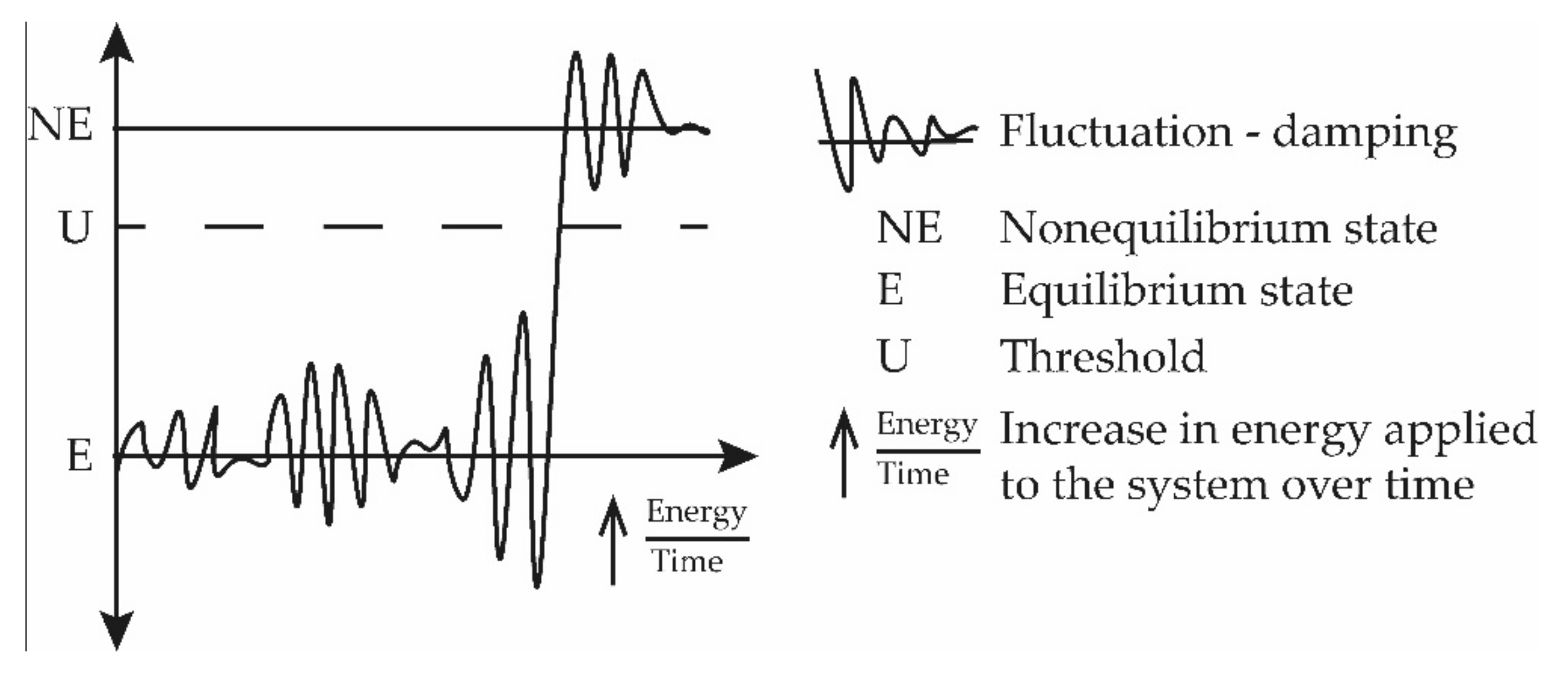
Prigogine observed that, far from the equilibrium situation, new ordered structures spontaneously arise [30] that require an input of energy to be preserved. However, they do not maintain linear relationships and are not possible to predict with current tools, precisely because of their nonlinear nature, as it occurs with the atmospheric interaction at ground level [31]. Close to the point where dissipative structures are organized, large fluctuations are observed that, instead of being dampened, can expand throughout the system, leading to new situations that are qualitatively very different from those that are close to equilibrium. It is necessary to distinguish equilibrium conditions (E), nonequilibrium conditions (NE), the process that leads from one to the other and the threshold (U) that separates both, as described qualitatively in Figure 1: initially, there are E (whatever these are) in which fluctuations occur with respect to said conditions that are dampened over time. If energy is supplied to the system, the fluctuations become large, but the system still manages to dampen them, until a point is reached where a certain threshold is exceeded, U. The fluctuation is no longer damped but stabilizes in a state far from the original equilibrium but equally stable as long as the energy supply continues, that is, a dissipative structure [4,32]. The dissipative structure, at the level of the earth’s surface, may have as one of its origins the Kolmogorov cascade [33]. The cascade supplies energy that favors the formation of unstable and turbulent structures near the surface.

Figure 1.
Dynamics of dissipative structures [34].
2.2. Tools for Analysis in Nonlinear Time Series
The Lyapunov exponent (λ) is defined as [2]:
where N is the number of iterations. That is, if two points of an orbit are initially very close to each other, this exponent is calculated for a large N. If after N iterations the points separate, this will be an indication of possible chaos in such a system. A positive value of the maximum Lyapunov exponent indicates chaos [2]. For a given time series, the sum of all the positive Lyapunov exponents defines its entropy SK and its reciprocal, the average predictability time, TP = 1/SK [34,35,36,37]. In practice, the Lyapunov exponent is obtained from this equation at the limit of a large N, for which saturation is evident. For stability of the calculation of the Lyapunov exponents, it is necessary to have over 5000 data points [38]. On the other hand, the correlation entropy [2,4] is defined as:
where C (m, r) is the correlation integral of the reconstructed path of a time series, m is the embedding or embedding dimension and r is the radius of the circle whose center is on an object that is composed of discrete points (in dimensions greater than two, the circles transform into (hyper) spheres). K2 is zero, positive or infinity for regular, chaotic or random data, respectively. A method to estimate K2 for experimental data is based on Grassberger and Procaccia [39]. These relationships were part of the numerical calculation procedure applied to each time series (for both pollutants and meteorological variables).
It is also possible to analyze the time series from another point of view, using the Hurst exponent, H. Through the fractal dimension, the roughness of the time series is analyzed, allowing to describe objects that present a high degree of complexity, comparing them according to the study periods. There are two attributes of great relevance in the study of fractal geometry, such as the Hurst exponent and the fractal or Mandelbrot dimension. These attributes are related to the degree of roughness that the time series can present. The fractal or Mandelbrot dimension, D = 2 − H, is a statistical quantity that allows one to mathematically describe objects that present a high degree of complexity, self-similarity or chaos. With the estimation of the Hurst exponent and the fractal dimension of the time series, it is possible to analyze whether a time series is fractal and to check if it has memory. If 0.5 < H < 1, these are time series that present persistence or correlated processes (one growth period is followed by a similar one) and have a smooth appearance. A persistent time series is characterized by long-term memory effects. Theoretically, what happens in the present will affect the future forever, and all current changes are correlated with all future changes. Persistent series are the most common in nature (black noise). In the case of the present study, it means that the time series were persistent, since every Hurst exponent was greater than 0.5 and less than 1. This condition implies that they have memory and similar behaviors in the future (greater probability that the increase in values is followed by an increase in short-term values and a decrease in values is more likely to be followed by a decrease in short-term values) and indicates that in the long term they could have the same trend or that they may repeat this behavior in the future. The determination of the Hurst exponent is a statistical method used to deduce the properties of a time series without making assumptions regarding their stationarity. The correlation dimension, DC > 5 essentially implies random data, which did not occur in this study.
The iterated function systems (IFS) fragmentation test also suggests a method of analysis of the data under study. The use of symbolic dynamics [40] allows one to calculate the Lempel–Ziv (LZ) complexity relative to white noise. When the data are chaotic, they are distributed forming, on a surface, localized groups [4]. In this condition, 0 < LZ < 1. Symbolic dynamics allows a simpler description of a complex behavioral dynamics system, which can be modeled directly. Information loss can be calculated according to:
where λ is the Lyapunov exponent and <ΔI> in (bits/h) is the loss of information. Two types of <ΔI> were calculated: one for the sum of the contribution of each P (pollutants: PM10, PM2.5 and CO) and another for the sum of the contribution of each MV (meteorological variables: T, WV, RH).
3. Materials and Methods
3.1. Area of Study
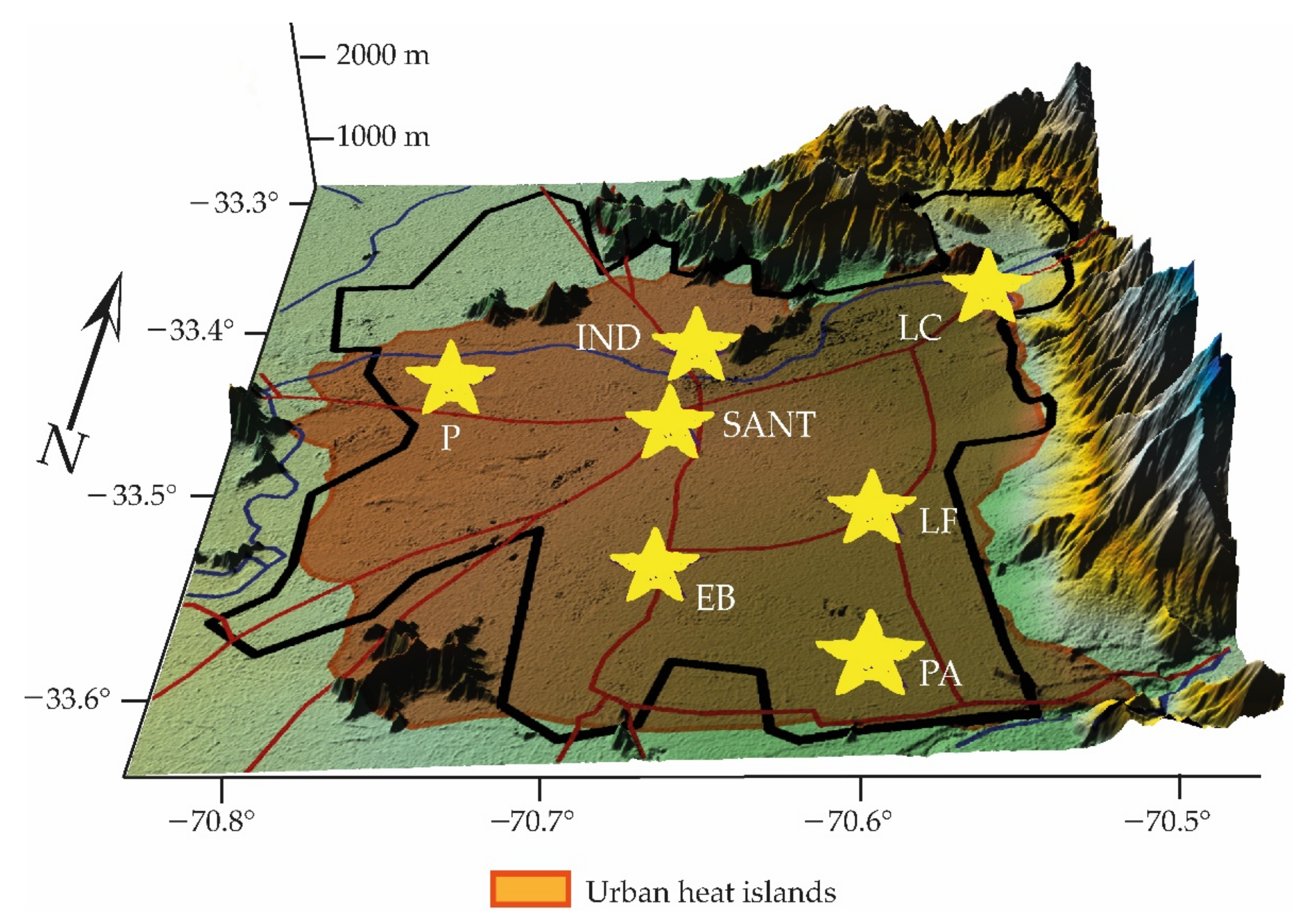
This study analyzed hourly time series data (each with 17,976 data points) from seven monitoring stations in the city of Santiago, Chile. The selected pollutants were PM10/PM2.5 and ground-level ozone (O3). The location of these stations is shown in Figure 2. At these stations, meteorological data such as temperature (T), wind speed (WS) and relative humidity (RH) were also measured. The data were obtained from the Air Quality National Information System [5,41] (42 time series, tested as chaotic, with a total of 754,992 data points on pollutants and meteorological variables).
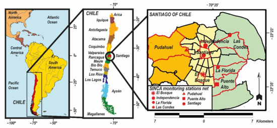
Figure 2.
Metropolitan area of Santiago communal map with their monitoring stations.
Table 1 contains the main physical, climatic, geographic, pollution and meteorological variables of the study sites shown in Figure 2.

Table 1.
For each locality studied, information on station name (with SINCA code in capital letters and meters above sea level (masl)), geography, climate, pollution, dominant wind direction (W), annual average temperature (T) and annual average relative humidity (RH%).
3.2. The Data
To study the effect of urban densification and micrometeorology on the sustainability of a coronavirus-type pandemic, a new set of time series was constructed from the information of patients infected and accumulated with SAR-COV-2 (AS) in the seven communes of the study (for the same period of 25 months: 30 March 2020 to 18 April 2022) [42]. The six new time series, by commune, were made up of the ratio of accumulated patients with meteorological and polluting variables: X = AS/T, Y = AS/WS, Z = AS/RH, U = AS/PM2.5, W = AS/PM10 and V = AS/O3 (with a total of 754,992 new data points for the seven communes).
3.2.1. PM2.5 and PM10 Particulate Matter
Of the vast existing documentation on these pollutants [43,44] of interest, a common aspect is their harmful effects on human health. These range from irritation in the respiratory tract, deposition in the lungs, which causes diseases such as silicosis and asbestosis, as well as worsening asthma and cardiovascular and respiratory diseases. In addition, all types of surfaces (housing, public sculptures, etc.) experience deterioration. Particulate matters also affect vegetation by interfering with photosynthesis. In the environment, they decrease visibility and induce cloud formation [45]. The World Health Organization [29] recommends for coarse particles (PM10) 20 µg m–3 as an annual average and 50 µg m–3 as an average in 24 h; for PM2.5, 10 µg m–3 as an annual average and 25 µg m–3 as an average in 24 h.
3.2.2. Tropospheric Ozone (O3)
This is a powerful oxidant that produces adverse effects on human health. Recent studies [46] have shown that O3 concentrations have adverse effects on respiratory function—especially in the summer—causing lung inflammation, respiratory failure, asthma and other bronchopulmonary diseases. European research [46] has shown that daily mortality increases with increasing exposure to ozone. New evidence links long-term exposure to ozone with greater effects on the deterioration of reproductive health and mortality [46]. Since 2005, several cohort analyses of long-term ozone exposure and respiratory mortality have been published. Evidence has emerged in studies [47] on cohorts and mortality of people with pre-existing diseases (chronic obstructive pulmonary disease (COPD), diabetes, heart failure, heart attack, etc.). In addition to its impacts on human health, vegetation and crops, ozone is currently considered the third most important greenhouse gas (after carbon dioxide and methane). According to the WHO, the eight-hour daily average concentration for tropospheric ozone is 100 µg m–3.
The selection of ozone (O3) was based on the fact that it has an adverse effect on the respiratory system of the inhabitants. In addition, it generates a picture of pre-existing diseases before the advent of COVID-19. On the other hand, in the Metropolitan Region, there is a connected urban meteorology that arises from urban heat islands (Figure 3) and urban canyons, as well as from the basin geography of the area. There are many local climatic zones depending on the size and complexity of the city. Therefore, the sectors can be recognized according to their predominant socioecological characteristics. These sectors make up socially constructed climates based on the socioeconomic levels of their inhabitants. They can be very connected with their interior and/or exterior, favoring the spread of a disease [4,48].

Figure 3.
RM communal map with the approximate location (darkest area) of the thermal island (SANT: Santiago, LC: Las Condes, LF = La Florida, PA = Puente Alto, P = Pudahuel, EB = El Bosque, IND = Independence).
3.2.3. Meteorological Variables
Time series of temperature (T), relative humidity (RH) and magnitude of wind speed (WS) were used in this study, allowing us to describe various atmospheric processes and their thermodynamics [12]. In the case of the Metropolitan Region (RM), there was also an influence from the orography of the area and the localized urban climate [41]. Table 2 presents the measuring instruments and their characteristics:

Table 2.
For the localities studied, information on the instruments for measuring pollutants and the instruments for measuring meteorological variables.
The conditions for using data provided the main following limitations: 1. have time series with valid data and measured with certified instruments; 2. if series with missing data are used (less than 5% of the total data of the series), the Kriging method [49] of filling in time series was applied to missing data; 3. series with a large number of data must be used to determine the highest Lyapunov exponent, for reasons of stability in the calculation procedure, which requires, ideally, over 5000 samples for each variable.
3.2.4. COVID-19 in Santiago de Chile
Waves
The study period covered 25 months, from 31 March 2020 to 18 April 2022. This time corresponded to a stage of rapid growth of the pandemic (which included three decreasing contagion waves over time until the end of 2021) in the Metropolitan Region [42] (Figure 4).
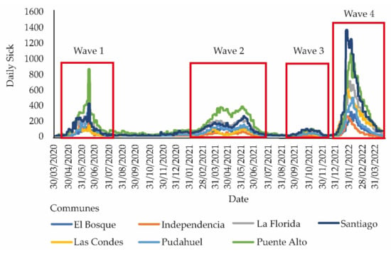
Figure 4.
Contagion waves consisting of maximum number of daily sick people, according to the seven communes. The rectangles framed in red are to visualize the waves and the period of occurrence.
The Metropolitan Region has a connected urban meteorology due to thermal islands (Figure 3) and urban canyons, apart from the basin geography that the area itself possesses. Many local climatic zones are present depending on the size and complexity of the Metropolitan Region. Thus, sectors can be recognized according to their predominant socioeconomical features (Appendix A, Table A1). These sectors make up socioclimates or socially constructed climates based on the socioeconomic levels of their inhabitants and can be highly connected to their interior, which favors the spread of a disease [48]. These antecedents allowed us to propose the study hypothesis: if a change in roughness is generated by high-rise construction and a high urban densification, then, together with urban micrometeorology and pollutants, a new thermal balance (thermal island) is achieved that makes the pandemic spread more effective.
Cumulative Sick Data
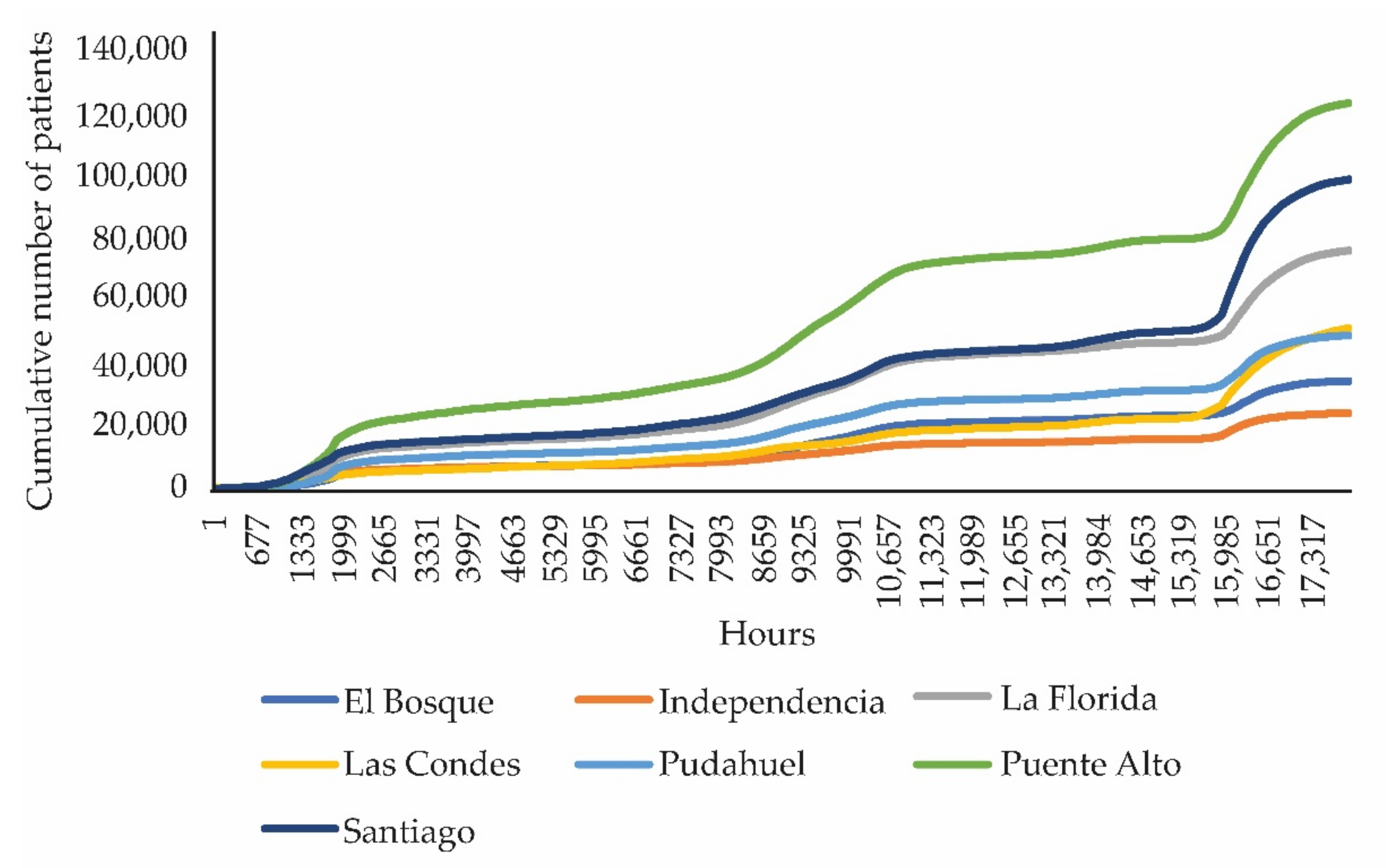
Figure 5 presents the accumulated number of patients by commune of the study in the period from 30 Mach 2020 to 18 April 2022.
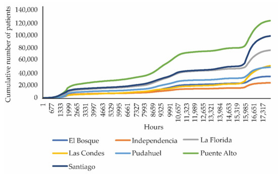
Figure 5.
Hourly accumulated sick people, at seven communes of the study period.
In the 2017 census, the Metropolitan Region had 7,037,000 inhabitants and the population of these seven communes represented approximately 30% of the entire population of Chile (for the year 2021, the projection of inhabitants for the Metropolitan Region was 7,987,723 inhabitants). Table 1 shows the population, accumulated patients, per capita income and multidimensional poverty index in the communes of the study. The analysis—through chaos theory—of the empirical data of meteorology and atmospheric pollutants, together with that of accumulated sick people (AS), provides relationships and connections between them. In addition, it provides general thermodynamic properties, such as entropy [50]. The accumulated sick people’s data were obtained from the Chilean Ministry of Health (MINSAL); they are summarized Table A1 (see Appendix A) and show the communes present in the study with their inhabitants, per capita income and multidimensional poverty index [4,51].
In [4], it was shown that if the pandemic (COVID-19) entered the human organism through the respiratory tract, then a connected urban meteorology promoted the sustainability and diffusion of pollutants. This, in turn, would make your actions more effective. In addition, it favored the infection, cultivation, and spread of this disease.
4. Results
The chaotic analysis [52] of the hourly time series X = AS/T, Y = AS/WS, Z = AS/RH, W = AS/PM10, U = AS/PM2.5 and V = AS/O3, each with 17,976 data points confirmed the hypothesis of this research that meteorology and pollutants can dissipate a pandemic by increasing its complexity. The IFS (iterated function systems) fragmentation test was fulfilled for the 42 series since 0 < LZ < 1, which is shown with the calculation for all communes in Table 3:

Table 3.
Nonlinear parameters [52] by commune and for accumulated sick people, meteorological variables and pollutants (period: 31 March 2020–18 April 2022).
The average predictability time () was calculated for the period under study and = 2.66 h was obtained, weighting the maximum average predictability times for the meteorological variables and for the pollutants of each of the seven communes. This average value coincides, approximately, with the viable stay of COVID-19 in aerosols indicated by Neeltje (3.00 h) [7]. In addition, it is of the order of the predictability time (3.07 h) [4] considering the three months of measurements, for accumulated patients, meteorological variables and pollutants.
In [4], it was shown, for a study period of 3 months (April to June 2020), that the communes with the highest number of accumulated sick people (Santiago (SANT), Puente Alto (PA), La Florida (LF)) were the ones that had the highest sum of partial entropies of each time series constructed from the quotient between hourly accumulated patients and each hourly time series of pollutants considered in this investigation (O3, PM2.5, PM10). This background made it necessary to study the effect of the change in roughness due to intensive urbanization and densification over a much longer period and its relationship with the districts with the highest number of accumulated sick people.
Let be the entropy of accumulated sick people by commune, with respect to the meteorological variables by commune, and the entropy of accumulated sick people per commune, with respect to the pollutants per commune. It is possible to calculate the sum of the entropies of the ratio between accumulated sick people/meteorological variables and the sum of the entropies of the ratio between accumulated sick people/pollutants. Then,
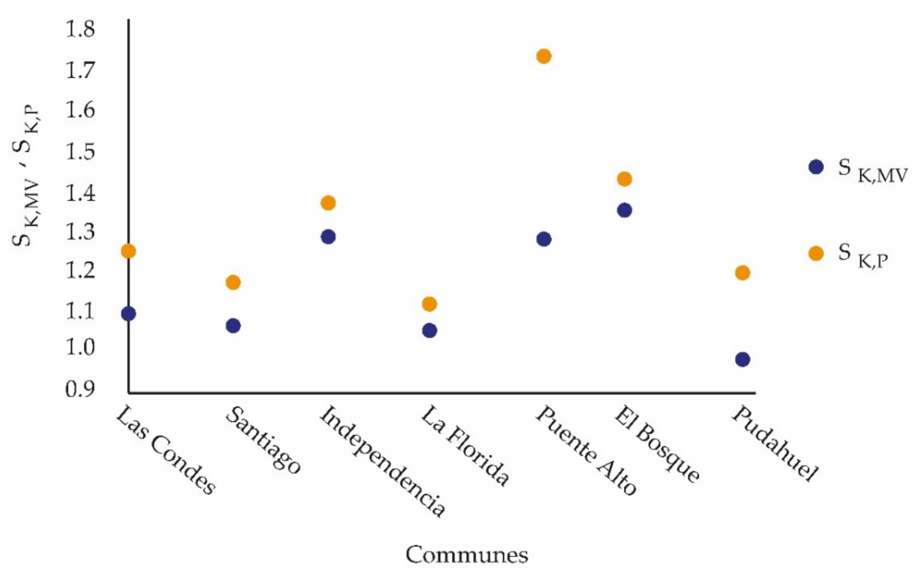
Figure 6 shows, comparatively, the sum of the entropies of the ratio between accumulated sick people/meteorological variables and the sum of the entropies of the ratio between accumulated sick people/pollutants.
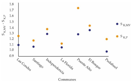
Figure 6.
Entropy for the quotient between accumulated sick people/localized climatology and accumulated sick people/pollutants, for each commune.
From Table 3, Figure 6 was obtained, from which it follows that SK, MV < SK, P. That is, the most entropic—those with the greatest connectivity in the city— are the pollutants. Figure 6 shows the influence exerted on the accumulated patients (of each commune) by their localized climatology (which is characterized by temperature, relative humidity and the magnitude of wind speed) and pollutants (PM2.5, PM10 and O3). In addition, it can be seen that those with the highest entropy are the pollutants, which, in turn, can favor the spread of the virus depending on the characteristics of the urban environment (roughness and densification).
Table 4 shows the communes with the greatest number of accumulated patients, and the ratio between the entropies of accumulated patients/meteorological variables and the entropies of accumulated patients/pollutants (SAS, MV/SAS, P). The pollutants influence the meteorological variables, which leads the system to a new equilibrium state that makes the virus more persistent.

Table 4.
Ratio between the entropies of accumulated patients/meteorological variables and the entropies of accumulated patients/pollutants and the accumulated sick people.
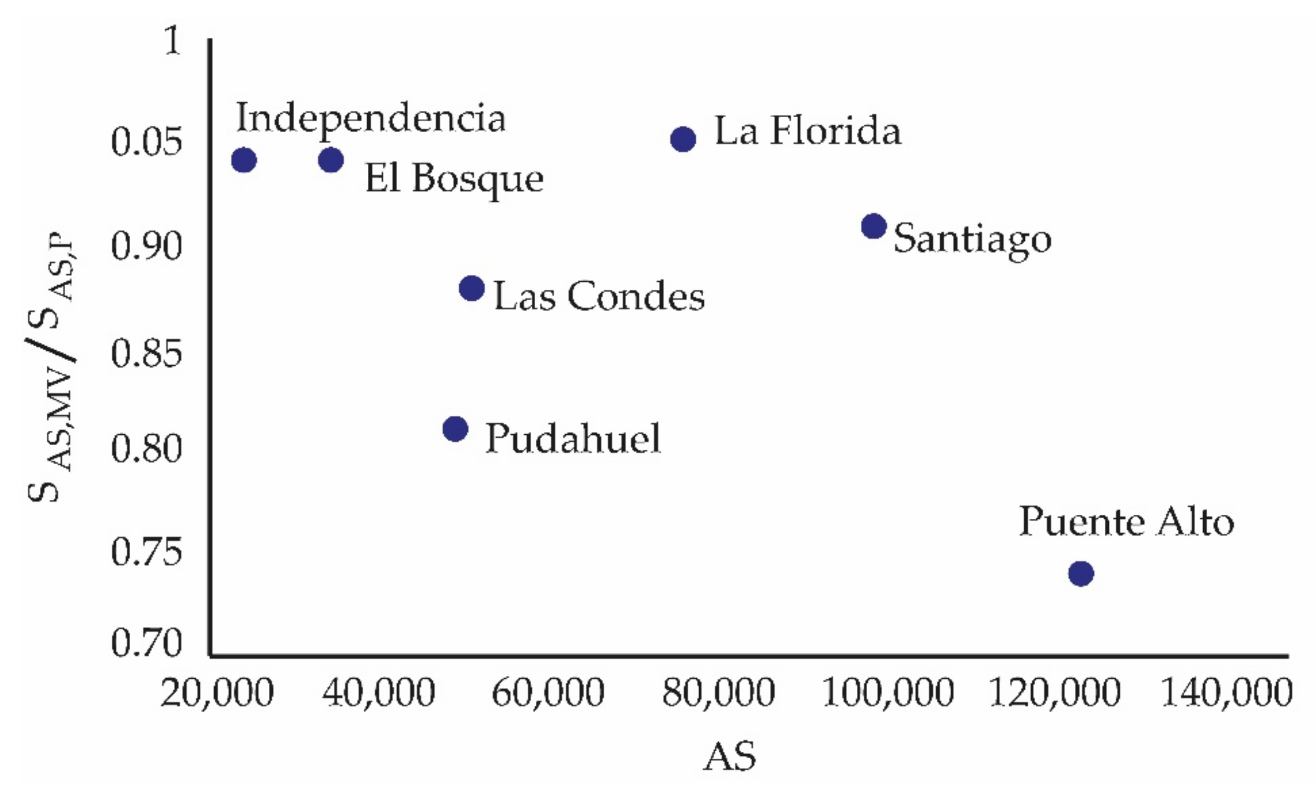
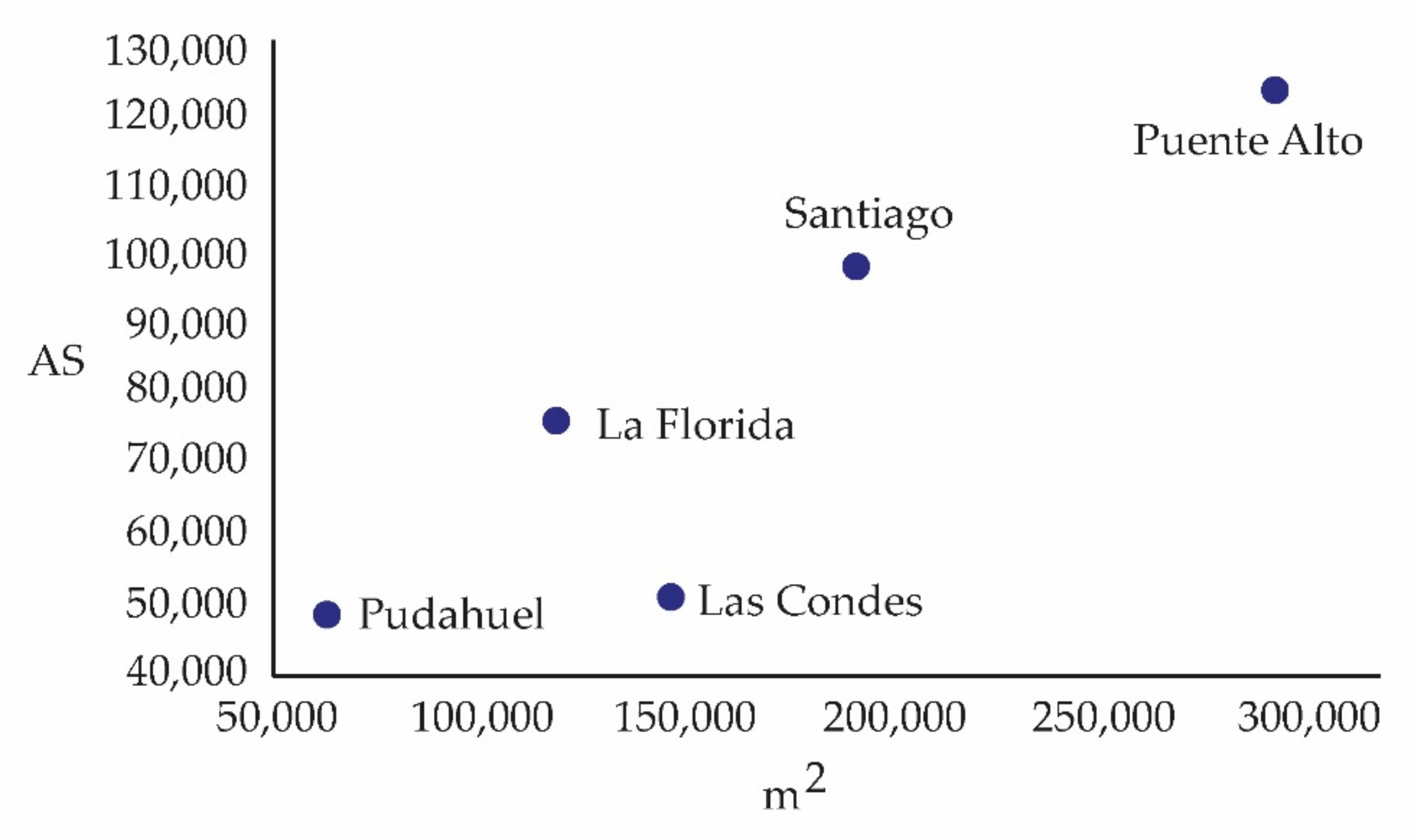
Figure 7 shows that there is a coincidence between the highest values of SAS, MV/SAS, P and the communes with the highest number of accumulated patients and those with the highest number of square meters built (this last statement is shown later). Thus, this extended study (31 March 2020, to 18 April 2022) again points to the same communes as in [4] as those that concentrate the largest number of accumulated patients. This is due to the fact that they have experienced an intense change in surface roughness due to high-rise construction and, as a consequence, a high urban densification [53,54], which continues to this day (Table 5 and Figure 8).

Figure 7.
Maximum ratios, between entropies of (accumulated patients)/(meteorological variables) and those of (accumulated patients)/(pollutants), SAS, MV/SAS, P, versus accumulated sick people (AS).

Table 5.
Approximate variation of square meters built in five communes of the study [27,28,42] and the accumulated sick people (2020–2022).

Figure 8.
Accumulated sick people (AS) by communes (5 of the 7 communes) and square meters built, in 2020.
The loss of information (Table 3, eighth column) from the system of meteorological variables and accumulated patients is greater compared to the system of pollutants and accumulated patients (Figure 9):
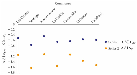
Figure 9.
Information loss for (accumulated patients)/(meteorological variables) () and information loss for (accumulated patients)/(pollutants) ( ) in the studied communes.
Calculating from Table 3 the averaged fractal dimension () [52] for (accumulated patients)/(meteorological variable), , and for (accumulated patients)/(pollutant), , for each commune, Table 6 is obtained:

Table 6.
Fractal dimension (D = 2 – H, with H, the Hurst exponent) can be averaged for accumulated sick/meteorological variable ( ) and for accumulated sick/pollutant ( ) for each commune. The fourth column represents the ratio between the third and second columns.
5. Discussion
In Table 3 (fifth column), the average of the Hurst coefficients was calculated. It was verified that the value of the (accumulated patients)/(meteorological variable) was less than of (accumulated patients)/(pollutants) for the same commune. Meteorological variables do not play such an active role in the ventilation of the city, as a result of the roughness due to high-rise construction, and the presence of pollutants (more persistent, greater ability to influence the future) in the air. This connects with an urban planning problem (UP). This was corroborated by calculating the Lempel–Ziv complexity averages (Table 3, sixth column). Once again, the urban Lempel–Ziv complexity favored pollutants, as indicated in Table 3 when comparing this chaotic parameter according to (accumulated patients)/(meteorological variable) for each commune, as it was lower than that of (accumulated patients)/(pollutants). If the city becomes progressively denser, localities within it can increase their density over others. If the localities are small, a random infection may affect only those localities. However, if the high-density locations are large, the infection will affect the entire system. Thus, there is an equilibrium density of built housing that can balance the infection. A critical state could be expected for which the buildings are barely disconnected throughout the city. Connectivity is an important property of complex systems [2,55]. Disease and infestation by virus would spread similarity to fire and in media other than forests, albeit at a slower rate [2,56]. In other words, urban micrometeorology appears to be affected in highly dense communes that show high rates of accumulated patients (Table 5).
According to Figure 8, the commune of Puente Alto (PA) was the one with the largest population in Chile and the one with the greatest Lempel–Ziv complexity of for the time series that represents the quotient (accumulated patients)/(temperature), which indicates a pre-existing condition of a high urban densification and that will affect the years to come. Moreover, as the uncertainty of climate behavior increases, according to Table 3, the communes studied showed a greater persistence (duration) in the ratio (accumulated patients)/(temperature), which was consistent with the persistent location of thermal islands [53,54]. This is also corroborated by the Hurst coefficient of these time series, which indicated the ability of the initial conditions to influence the future.
Figure 9 showed that UP favored the persistence of SK, P, since the loss of information was slower. There was a “historical cumulative anchorage (initial condition)” associated with the concentration of air pollutants. Its effects were felt on the accumulated patients in a shorter predictability time (2.505 h) when compared to that of SK, MV. UP affected the persistence of SK, MV (Figure 9) in the opposite way. The UP weakened the urban meteorology causing it to lose information faster. This embrittlement was long-range as indicated by the calculation of the predictability time associated with SK, MV (2.805 h). This is proof that a growing urbanization has a first order of priority in the action of making the permanence of the pandemic temporarily more sustainable. This has harmful implications for people’s health as it shows that air pollution has a certain stability over time.
The correlation dimension, in general, of the (accumulated patients)/(pollutant) time series was greater than the (accumulated patients)/(meteorological variables) time series (Table 3). Table 6 showed that the fractal dimension, , for all communes, was greater than the fractal dimension , which indicated a sensitivity to a change in roughness of the meteorological variables. The fractional dimension of the fractal object (Table 6) contained in the (accumulated patients)/(meteorological variables) time series was greater than the fractional dimension of the fractal object contained in the (accumulated patients)/(pollutant) time series. This showed that the time series of (accumulated patients)/(meteorological variables) was more chaotic. The roughness of the series was also affected by the change in the roughness of the soils due to intensive urbanization processes that led to urban densification from cases of densification in contexts that favored certain mitigation to other contexts of little or no influence (cruder). Intensive urbanization was in closer contact with localized micrometeorology. This means that the time series contained in its measurements this sensitivity to changes in the conditions of the environment (roughness), which affected the ventilation of the commune. The Puente Alto commune stood out for several reasons. Its forest cover is 20.3%. It was a peripheral commune of the Metropolitan Region, but today it is very connected to the center of Santiago. According to data from the 2017 Census [27], the commune had 568,106 inhabitants (the most populous in Chile), with many housing projects of tall buildings and one-story houses. This commune is partially affected by a geological fault, called San Ramón, which has been populated despite its status as a high-risk area.
6. Conclusions
From the databases used (1,509,984 data points) between the years 2020 and early 2022, to which a chaotic analysis was applied, it can be concluded that:
The time series of the ratios between (accumulated patients)/(meteorological variables) and (accumulated patients)/(pollutants) represented irreversible processes.
The entropies of the time series of (accumulated patients)/(pollutants) were greater than the entropies of the series of (accumulated patients)/(meteorological variables). The commune of Puente Alto, with an intensive housing construction process (Figure 8), the largest communal population in Chile and the largest number of accumulated patients in the metropolitan region, also presented the largest entropic gap (Figure 6) in favor of the contaminants. This contributes to its urban meteorology being very polluted and conditions that favor the spread of the virus.
The average value of the Hurst coefficient and the Lempel–Ziv complexity for the time series of (accumulated patients)/(pollutants) was greater than that of the time series of (accumulated patients)/(meteorological variable). This means more persistence and connectivity for contaminants. As Figure 9 showed, the loss of information of the contaminant on the accumulated patients is the slowest.
All the time series of (accumulated patients)/(meteorological variables) had a greater average fractal dimension than those of the time series of (accumulated patients)/(pollutants) (Table 6). The communes studied were in a process of changing the roughness of their surface due to the construction of high-rise buildings. The case that stood out was the commune of Puente Alto, a commune with the highest population growth in Chile and with the highest number of accumulated patients. Its high fractal dimension showed a sensitivity of its urban meteorology to intensive changes in surface roughness (formation of urban canyons, poorly ventilated sectors, etc.)
The time series of (accumulated patients)/(temperature meteorological variable) showed a greater Lempel–Ziv complexity with respect to the other meteorological variables, which was consistent with the presence of thermal islands. It also showed, in most cases, a greater persistence: the past influenced the future.
The average time of predictability of pandemic propagation in communes whose urban meteorology was subjected to atmospheric pollution and population densification processes was comparable to that obtained under controlled experimental conditions. The chaotic parameters of the time series, which contain information on the interactions between urban meteorology, pollutants, accumulated patients, showed that intensive urbanization processes can make the pandemic sustainable.
Future Lines of Research
The authors have developed another line of research that is related to the geographic geomorphologies where the cities are located: basin, coast and mountain. The authors have proven, in an article about to be submitted to a journal, that urban meteorology, pollutants and urbanization are related differently depending on where the city is located. Santiago de Chile, the place of the study sent to Atmosphere, is a basin. It is of interest to comparatively analyze how the sustainability of the pandemic manifests itself in other geographical configurations.
Author Contributions
Conceptualization, P.P.; methodology, P.P. and E.M.; software, P.P.; validation, P.P. and E.M.; formal analysis, P.P.; investigation, P.P.; resources, E.M.; data curation, E.M.; writing—original draft preparation, P.P.; writing—review and editing, P.P. and E.M.; visualization, E.M.; supervision, P.P.; project administration, P.P.; funding acquisition, P.P. All authors have read and agreed to the published version of the manuscript.
Funding
This research received no external funding.
Institutional Review Board Statement
Not applicable.
Informed Consent Statement
Informed consent was obtained from all subjects involved in the study.
Data Availability Statement
The data were obtained from the public network for online monitoring of air pollutant concentration and meteorological variables. The network is distributed throughout Chile, without access restrictions. It is under the responsibility of SINCA, the National Air Quality Information System, dependent on the Environment Ministry of Chile [5,41]. The data for the two study periods will be available for free use on the Web page: URL: https://sinca.mma.gob.cl (accessed on 23 April 2022). The health data were obtained from [6,42].
Acknowledgments
The authors gratefully acknowledge the Direction for Research that funded this study through Project LPR20-02 and the Department of Physics, both part of Universidad Tecnológica Metropolitana.
Conflicts of Interest
The authors declare no conflict of interest.
Abbreviations
| T | Temperature |
| RH | Relative humidity |
| WS | Wind speed magnitude |
| PM2.5 | 2.5-micrometer particulate matter |
| PM10 | 10.0-micrometer particulate matter |
| 03 | Tropospheric ozone |
| SINCA | Chilean Air Quality National Information System |
| MINSAL | Chilean Ministry of Health |
| MVU | Ministry of housing and urbanism of Chile |
| INE | National Statistics Institute of Chile |
| WHO | World Health Organization |
| SANT | Santiago (Used by SINCA: EMN) |
| LC | Las Condes (Used by SINCA: EMM) |
| LF | La Florida (Used by SINCA: EML) |
| PA | Puente Alto (Used by SINCA: EMS) |
| P | Pudahuel (Used by SINCA: EMO) |
| EB | El Bosque (Used by SINCA: EMQ) |
| IND | Independencia (Used by SINCA: EMF) |
| AS | Accumulated sick people |
| X = AS/T | Time series of (hourly accumulated patients)/(hourly temperature) |
| Y = AS/WS | Time series of (hourly accumulated patients)/(hourly magnitude of the wind speed) |
| Z = AS/RH | Time series of (hourly accumulated patients)/(hourly relative humidity) |
| W = AS/PM10 | Time series of (hourly accumulated patients)/(hourly PM10 particulate matter) |
| U = AS/PM2.5 | Time series of (hourly accumulated patients)/(hourly PM2.5 particulate matter) |
| V = AS/O3 | Time series of (hourly accumulated patients)/(hourly tropospheric ozone) |
| SK,MV | Entropy of time series of (hourly accumulated patients)/(hourly meteorological variables) |
| SK,P | Entropy of time series of (hourly accumulated patients)/(hourly pollutants) |
| λ | Lyapunov coefficient |
| DC | Correlation dimension |
| SK | Correlation entropy |
| LZ | Lempel–Ziv complexity |
| H | Hurst coefficient |
| DAS/MV | The averaged fractal dimension of time series of (hourly accumulated patients)/(hourly meteorological variable) |
| DAS/P | The averaged fractal dimension of time series of (hourly accumulated patients)/(hourly pollutants) |
| <ΔI>MV | Loss of information from the system (accumulated patients)/(meteorological variable) |
| <ΔI>P | Loss of information from the system (accumulated patients)/(pollutants) |
Appendix A

Table A1.
Studied communes and population according to 2017 [27]. Each statement separated by a comma corresponds to a column of data.
Table A1.
Studied communes and population according to 2017 [27]. Each statement separated by a comma corresponds to a column of data.
| Communes, Population by Commune (2017), Accumulated Sick (31 March 2020–18 April 2022), People Per Capita Income (In US), Multidimensional Poverty Index | ||||
|---|---|---|---|---|
| Santiago | 404,496 | 98,653 | 471 | 5–10% |
| Independencia | 100,281 | 24,082 | 127 | 20–25% |
| Las Condes | 294,838 | 51,154 | 1317 | <5% |
| Puente Alto | 568,106 | 123,045 | 175 | 20–25% |
| El Bosque | 162,505 | 34,385 | 188 | 20–25% |
| La Florida | 366,916 | 75,964 | 209 | 15–20% |
| Pudahuel | 230,293 | 48,900 | 335 | 20–25% |
| Total | 2,127,435 | 456,183 | / | / |
References
- Earn, D.J.D.; Rohani, P.; Bolker, B.M.; Grenfell, B.T. A Simple Model for Complex Dynamical Transitions in Epidemics. Science 2000, 287, 667–670. [Google Scholar] [CrossRef] [PubMed]
- Sprott, J.C. Chaos and Time-Series Analysis, 1st ed.; Oxford University Press: Oxford, UK, 2003. [Google Scholar]
- Baker, R.E.; Yang, W.; Vecchi, G.A.; Metcalf, C.J.E.; Grenfell, B.T. Susceptible supply limits the role of climate in the COVID-19 pandemic. Science 2020, 369, 315–319. [Google Scholar] [CrossRef] [PubMed]
- Salini, G.A.; Pacheco, P.R.; Mera, E.; Parodi, M.C. Probable Relationship between COVID-19, Pollutants and Meteorology: A Case Study at Santiago, Chile. Aerosol Air Qual. Res. 2021, 21, 200434. [Google Scholar] [CrossRef]
- Chilean Air Quality National Information System (SINCA). Available online: https://sinca.mma.gob.cl (accessed on 30 April 2022).
- Chilean Ministry of Health (MINSAL). Available online: https://www.minsal.cl/ (accessed on 30 April 2022).
- Van Doremalen, N.; Bushmaker, T.; Morris, D.H.; Holbrook, M.G.; Gamble, A.; Williamson, B.N.; Tamin, A.; Harcourt, J.L.; Thornburg, N.J.; Gerber, S.I.; et al. Aerosol and Surface Stability of SARS-CoV-2 as Compared with SARS-CoV-1. N. Engl. J. Med. 2020, 382, 1564–1567. [Google Scholar] [CrossRef]
- Tang, J.; Bahnfleth, W.; Bluyssen, P.; Buonanno, G.; Jimenez, J.; Kurnitski, J.; Li, Y.; Miller, S.; Sekhar, C.; Morawska, L.; et al. Dismantling myths on the airborne transmission of severe acute respiratory syndrome coronavirus-2 (SARS-CoV-2). J. Hosp. Infect. 2021, 110, 89–96. [Google Scholar] [CrossRef]
- Fears, A.C.; Klimstra, W.B.; Duprex, P.; Hartman, A.; Weaver, S.C.; Plante, K.S.; Mirchandani, D.; Plante, J.A.; Aguilar, P.V.; Fernández, D.; et al. Persistence of Severe Acute Respiratory Syndrome Coronavirus 2 in Aerosol Suspensions. Emerg. Infect. Dis. 2020, 26, 2168–2171. [Google Scholar] [CrossRef]
- Hamner, L.; Dubbel, P.; Capron, I.; Ross, A.; Jordan, A.; Lee, J.; Lynn, J.; Ball, A.; Narwal, S.; Russell, S.; et al. High SARS-CoV-2 Attack Rate Following Exposure at a Choir Practice—Skagit County, Washington, March 2020. MMWR Morb. Mortal. Wkly. Rep. 2020, 69, 606–610. [Google Scholar] [CrossRef]
- Stadnytskyi, V.; Bax, C.E.; Bax, A.; Anfinrud, P. The airborne lifetime of small speech droplets and their potential importance in SARS-CoV-2 transmission. Proc. Natl. Acad. Sci. USA 2020, 117, 11875–11877. [Google Scholar] [CrossRef]
- Iqbal, N.; Fareed, Z.; Shahzad, F.; He, X.; Shahzad, U.; Lina, M. The nexus between COVID-19, temperature and exchange rate in Wuhan city: New findings from partial and multiple wavelet coherence. Sci. Total Environ. 2020, 729, 138916. [Google Scholar] [CrossRef]
- Neiderud, C.-J. How urbanization affects the epidemiology of emerging infectious diseases. Infect. Ecol. Epidemiol. 2015, 5, 27060. [Google Scholar] [CrossRef]
- Martínez, L.; Short, J. The Pandemic City: Urban Issues in the Time of COVID-19. Sustainability 2021, 13, 3295. [Google Scholar] [CrossRef]
- Mouratidis, K.; Yiannakou, A. COVID-19 and urban planning: Built environment, health, and well-being in Greek cities before and during the pandemic. Cities 2021, 121, 103491. [Google Scholar] [CrossRef]
- McConnell, P.J. COVID-19 Pandemic—A Systems Thinking Approach. SSRN. 2021. Available online: https://ssm.com/abstract=3972869 (accessed on 4 March 2022). [CrossRef]
- Bradley, D.T.; Mansouri, M.A.; Kee, F.; Garcia, L.M.T. A systems approach to preventing and responding to COVID-19. eClinicalMedicine 2020, 21, 100325. [Google Scholar] [CrossRef]
- Zhao, W.; Zhang, J.; Meadows, M.E.; Liu, Y.; Hua, T.; Fu, B. A systematic approach is needed to contain COVID-19 globally. Sci. Bull. 2020, 65, 876–878. [Google Scholar] [CrossRef]
- Sahin, O.; Salim, H.; Suprun, E.; Richards, R.; MacAskill, S.; Heilgeist, S.; Rutherford, S.; Stewart, R.A.; Beal, C.D. Developing a Preliminary Causal Loop Diagram for Understanding the Wicked Complexity of the COVID-19 Pandemic. Systems 2020, 8, 20. [Google Scholar] [CrossRef]
- Nieto-Chaupis, H. Identifying Second Wave and New Variants of Covid-19 from Shannon Entropy in Global Pandemic Data. In Proceedings of the 2021 Fifth World Conference on Smart Trends in Systems Security and Sustainability (WorldS4), London, UK, 29–30 July 2021. [Google Scholar] [CrossRef]
- Mauree, D.; Coccolo, S.; Deschamps, L.; Loesch, P.; Becquelin, P.; Scartezzini, J.-L. Mobile Urban Micrometeorological Monitoring (MUMiM). J. Phys. Conf. Ser. 2019, 1343, 12014. [Google Scholar] [CrossRef]
- Foken, T. Micrometeorology; Springer: Berlin/Heidelberg, Germany, 2008. [Google Scholar]
- Klausner, Z.; Ben-Efraim, M.; Arav, Y.; Tas, E.; Fattal, E. The Micrometeorology of the Haifa Bay Area and Mount Carmel during the summer. Atmosphere 2021, 12, 354. [Google Scholar] [CrossRef]
- Stull, R.B. Introduction to Boundary Layer Meteorology; Kluwer Academic: Alphen aan den Rijn, The Netherlands, 1988; 666p. [Google Scholar]
- Fattal, E.; David-Saroussi, H.; Klausner, Z.; Buchman, O. An Urban Lagrangian Stochastic Dispersion Model for Simulating Traffic Particulate-Matter Concentration Fields. Atmosphere 2021, 12, 580. [Google Scholar] [CrossRef]
- Garratt, J.R.; Pearman, G.I. Retrospective Analysis of Micrometeorological Observations Above an Australian Wheat Crop. Bound.-Layer Meteorol. 2020, 177, 613–641. [Google Scholar] [CrossRef]
- INE-Plataforma de Datos Estadísticos. Available online: https://www.ine.cl/docs/default-source/encuesta-suplementaria-de-ingresos/publicaciones-y-anuarios/sntesis-de-resultados/2019/síntesis-nacional-esi-2019.pdf (accessed on 4 January 2022).
- MVU, Ministerio de Vivienda y Urbanismo (Ministry of Housing and Urbanism); Centro de Estudios de Ciudad y Territorio. Available online: https://www.observatoriourbano.cl (accessed on 3 January 2022).
- WHO. Europe 2013. Review of Evidence on Health Aspects of Air Pollution—REVIHAAP Project Technical Report, World Health Organization, Regional Office for Europe, Copenhagen, Denmark. Available online: https://www.eea.europa.eu/data-and-maps/indicators/exceedance-of-air-quality-limit-3/who-2013 (accessed on 10 September 2021).
- Eckert, K.; Bestehorn, M.; Thess, A. Square cells in surface-tension-driven Bénard convection: Experiment and theory. J. Fluid Mech. 1998, 356, 155–197. [Google Scholar] [CrossRef]
- Richardson, L.F. Weather Prediction by Numerical Process; Cambridge University Press: Cambridge, UK, 1922. [Google Scholar]
- Manriquez, R. Estructuras disipativas. De la termodinámica a la psicoterapia familiar. Rev. Asoc. Esp. Neuropsiquiatría 1987, 7, 435–454. [Google Scholar]
- Kolmogorov, A.N. The local structure of turbulence in incompressible viscous fluid for very large Reynolds FV. Dokl. Akad. Nauk. SSSR 1941, 30, 301–305. [Google Scholar]
- Pacheco, P.R.; Salini, G.A.; Mera, E.M. Entropía y neguentropía: Una aproximación al proceso de difusión de contami-nantes y su sostenibilidad. Rev. Int. Contam. Ambient. 2021, 37, 167–185. [Google Scholar]
- Lorenz, E. Deterministic nonperiodic flow. J. Atmos. Sci. 1963, 20, 130–141. [Google Scholar] [CrossRef]
- Salini-Calderón, G.-A.; Perez, P. A Study of the Dynamic Behaviour of Fine Particulate Matter in Santiago, Chile. Aerosol Air Qual. Res. 2015, 15, 154–165. [Google Scholar] [CrossRef]
- Chen, Y.; Wang, J.; Feng, J. Understanding the Fractal Dimensions of Urban Forms through Spatial. Entropy 2017, 19, 600. [Google Scholar] [CrossRef]
- Wolf, A.; Swift, J.B.; Swinney, H.L.; Vastano, J.A. Determining Lyapunov exponents from a time series. Phys. D Nonlinear Phenom. 1985, 16, 285–317. [Google Scholar] [CrossRef]
- Grassberger, P.; Procaccia, I. Characterization of Strange Attractors. Phys. Rev. Lett. 1983, 50, 346–349. [Google Scholar] [CrossRef]
- Horna, J.; Dionicio, J.; Martinez, R.; Zavaleta, A.; Brenis, Y. Dinámica simbólica y algunas aplicaciones. Sel. Mat. 2016, 3, 101–106. [Google Scholar] [CrossRef]
- Chilean Ministry of the Environment (MMA). Available online: https://sinca.mma.gob.cl/index.php (accessed on 30 April 2022).
- Government of Chile. Official Data COVID-19. Available online: https://www.gob.cl/coronavirus/cifrasoficiales/ (accessed on 30 April 2022).
- Gramsch, E.; Morales, L.; Baeza, M.; Ayala, C.; Soto, C.; Neira, J.; Pérez, P.; Moreno, F. Citizens’ Surveillance Micro-network for the Mapping of PM2.5 in the City of Concón, Chile. Aerosol Air Qual. Res. 2020, 20, 358–368. [Google Scholar] [CrossRef]
- Đorđević, D.; Đuričić-Milanković, J.; Pantelić, A.; Petrović, S.; Gambaro, A. Coarse, fine and ultrafine particles of sub-urban continental aerosols measured using an 11-stage Berner cascade impactor. Atmos. Pollut. Res. 2020, 11, 499–510. [Google Scholar] [CrossRef]
- Iwasaka, Y.; Minoura, H.; Nagaya, K. The transport and spacial scale of Asian dust-storm clouds: A case study of the dust-storm event of April 1979. Tellus B Chem. Phys. Meteorol. 1983, 35, 189–196. [Google Scholar] [CrossRef]
- Nuvolone, D.; Petri, D.; Voller, F. The effects of ozone on human health. Environ. Sci. Pollut. Res. 2017, 25, 8074–8088. [Google Scholar] [CrossRef] [PubMed]
- Díaz, J.; Ortiz, C.; Falcón, I.; Salvador, C.; Linares, C. Short-term effect of tropospheric ozone on daily mortality in Spain. Atmos. Environ. 2018, 187, 107–116. [Google Scholar] [CrossRef]
- Byass, P. Eco-epidemiological assessment of the COVID-19 epidemic in China, January–February 2020. Glob. Health Action 2020, 13, 1760490. [Google Scholar] [CrossRef]
- Silveman, B.W.; Jones, M.C.; Fix, E.; Hodges, J.L. An Important Contribution to Nonparametric Discriminant Analysis and Density Estimation. Int. Stat. Rev. 1951, 57, 233. [Google Scholar] [CrossRef]
- Pacheco, P.R.; Mera, E.M.; Salini, G.A. Medición Localizada de Contaminantes Atmosféricos y Variables Meteorológicas: Segunda Ley de la Termodinámica. Inf. Technol. 2019, 30, 105–116. [Google Scholar] [CrossRef][Green Version]
- Census. XIX Censo Nacional de Población y VIII de Vivienda o Censo de Población y Vivienda 2017, Gobierno de Chile e Instituto Nacional de Estadísticas de Chile. 2017. Available online: https://www.ine.cl (accessed on 23 November 2021).
- Sprott, J.C. Chaos Data Analyzer Software. Michigan, EEUU. 1995. Available online: https://sprott.physics.wisc.edu./cda.htm (accessed on 15 April 2020).
- Burra, P.; Soto-Díaz, K.; Chalen, I.; Gonzalez-Ricon, R.J.; Istanto, D.; Caetano-Anollés, G. Temperature and Latitude Correlate with SARS-CoV-2 Epidemiological Variables but not with Genomic Change Worldwide. Evol. Bioinform. 2021, 17, 1176934321989695. [Google Scholar] [CrossRef]
- Pacheco, P.; Mera, E.; Salini, G. Urban Densification Effect on Micrometeorology in Santiago, Chile: A Comparative Study Based on Chaos Theory. Sustainability 2022, 14, 2845. [Google Scholar] [CrossRef]
- Green, D.G. Connectivity and the evolution of biological systems. J. Biol. Syst. 1994, 2, 91–103. [Google Scholar] [CrossRef]
- Kesten, H. Percolation Theory and Ergodic Theory of Infinite Particle Systems; Springer: New York, NY, USA, 1987. [Google Scholar]
Publisher’s Note: MDPI stays neutral with regard to jurisdictional claims in published maps and institutional affiliations. |
© 2022 by the authors. Licensee MDPI, Basel, Switzerland. This article is an open access article distributed under the terms and conditions of the Creative Commons Attribution (CC BY) license (https://creativecommons.org/licenses/by/4.0/).

