
Applicability of a CEEMD–ARIMA Combined Model for Drought Forecasting: A Case Study in the Ningxia Hui Autonomous Region


Abstract
:1. Introduction
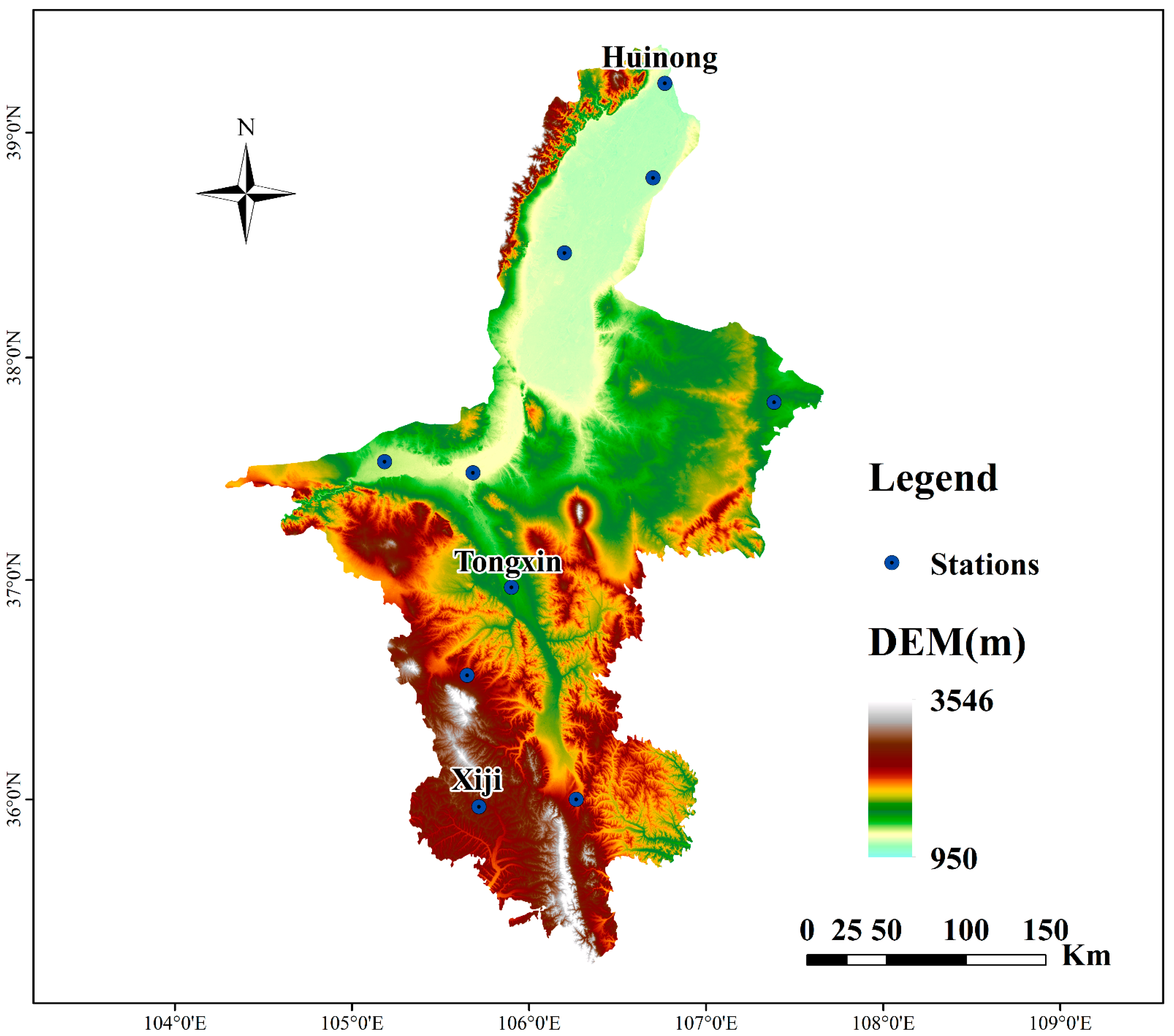
2. Study Area
3. Materials and Methods
3.1. Data Sources
3.2. Research Methods
3.2.1. SPI
3.2.2. ARIMA Model
3.2.3. CEEMD
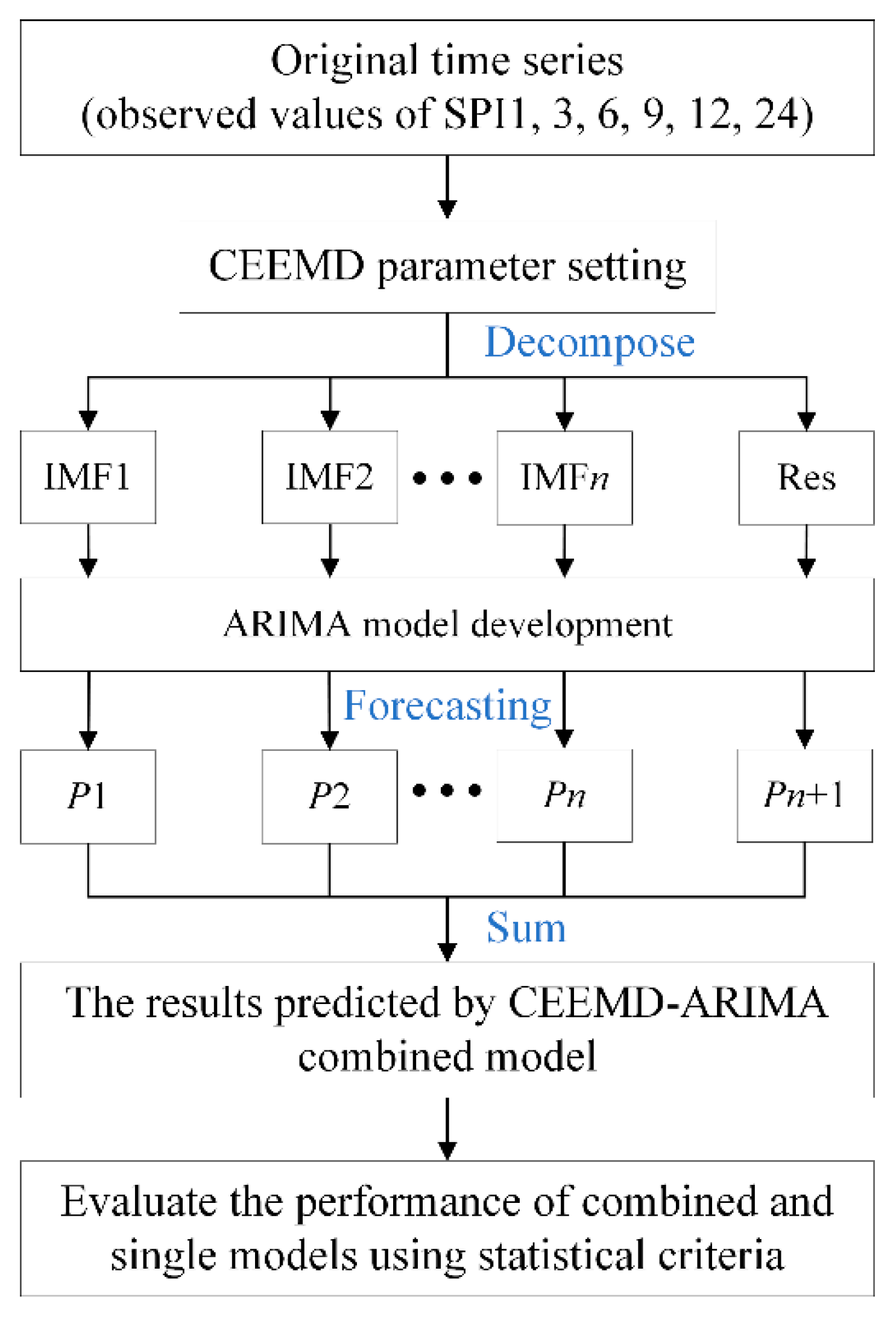
3.2.4. CEEMD–ARIMA Combined Model
3.2.5. Evaluation Index
4. Results
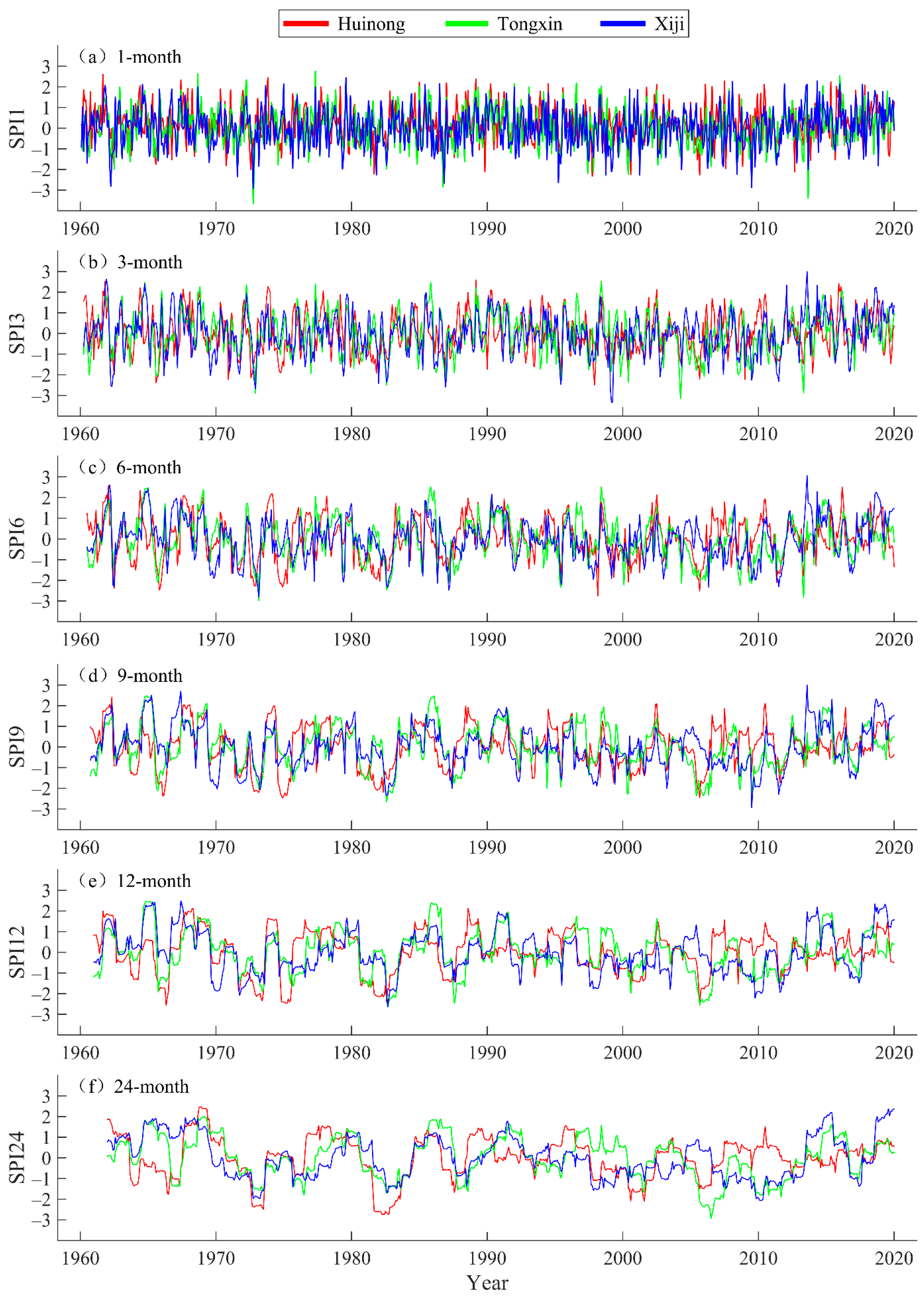
4.1. SPI Values at Different Time Scales
4.2. The ARIMA Modeling and Prediction
4.3. The CEEMD–ARIMA Combined Model
5. Discussion
6. Conclusions
- (1)
- As an effective nonlinear and nonstationary time-series decomposition method, CEEMD can extract the change trend of the SPI series and describe the characteristics of drought trends under climate change. Using CEEMD to decompose the SPI sequence of the Ningxia Hui Autonomous Region, seven IMF components and one trend item were obtained. The fluctuation of the component quantity became smoother than that of the original sequence, providing a basis for model prediction.
- (2)
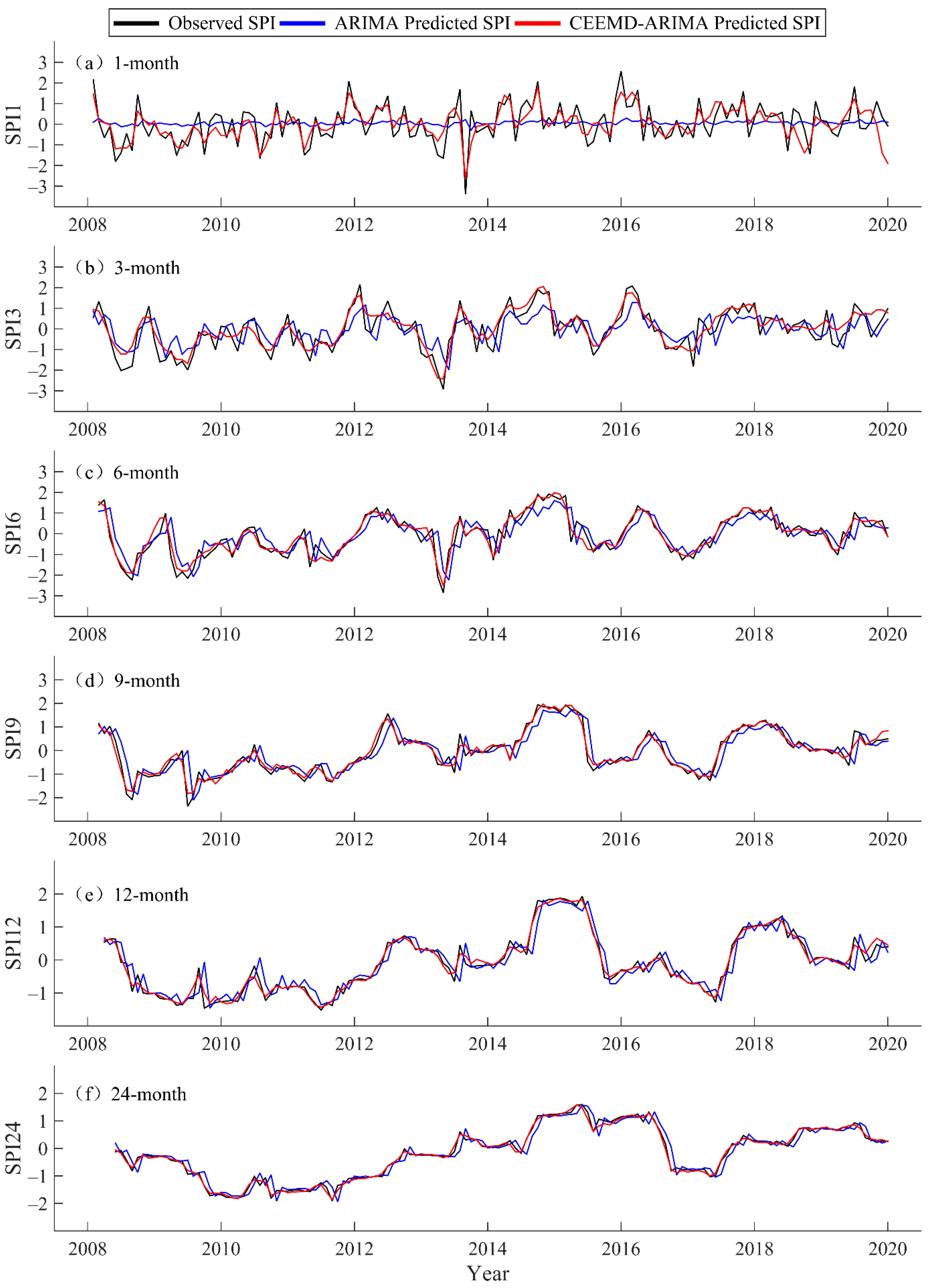
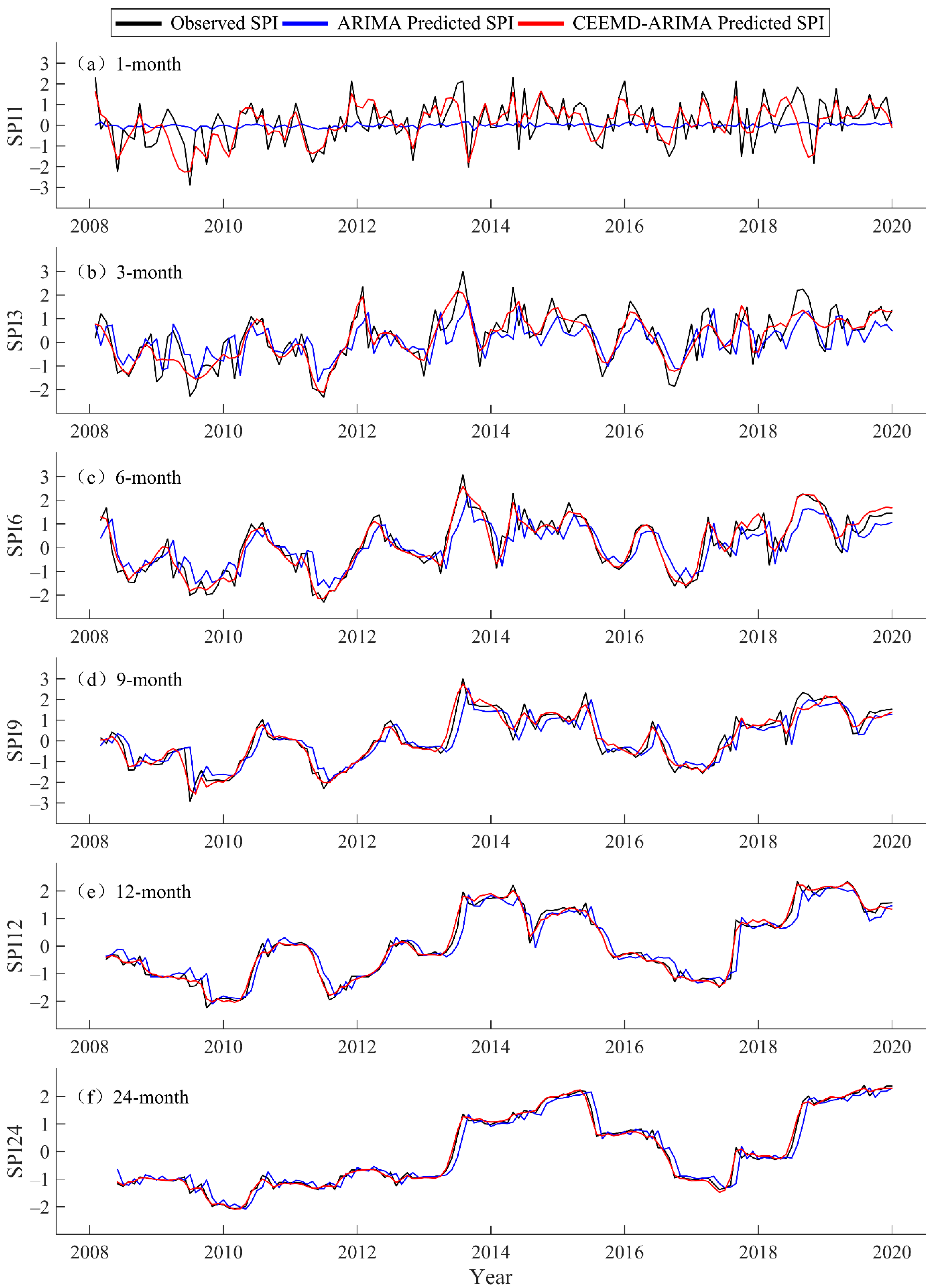
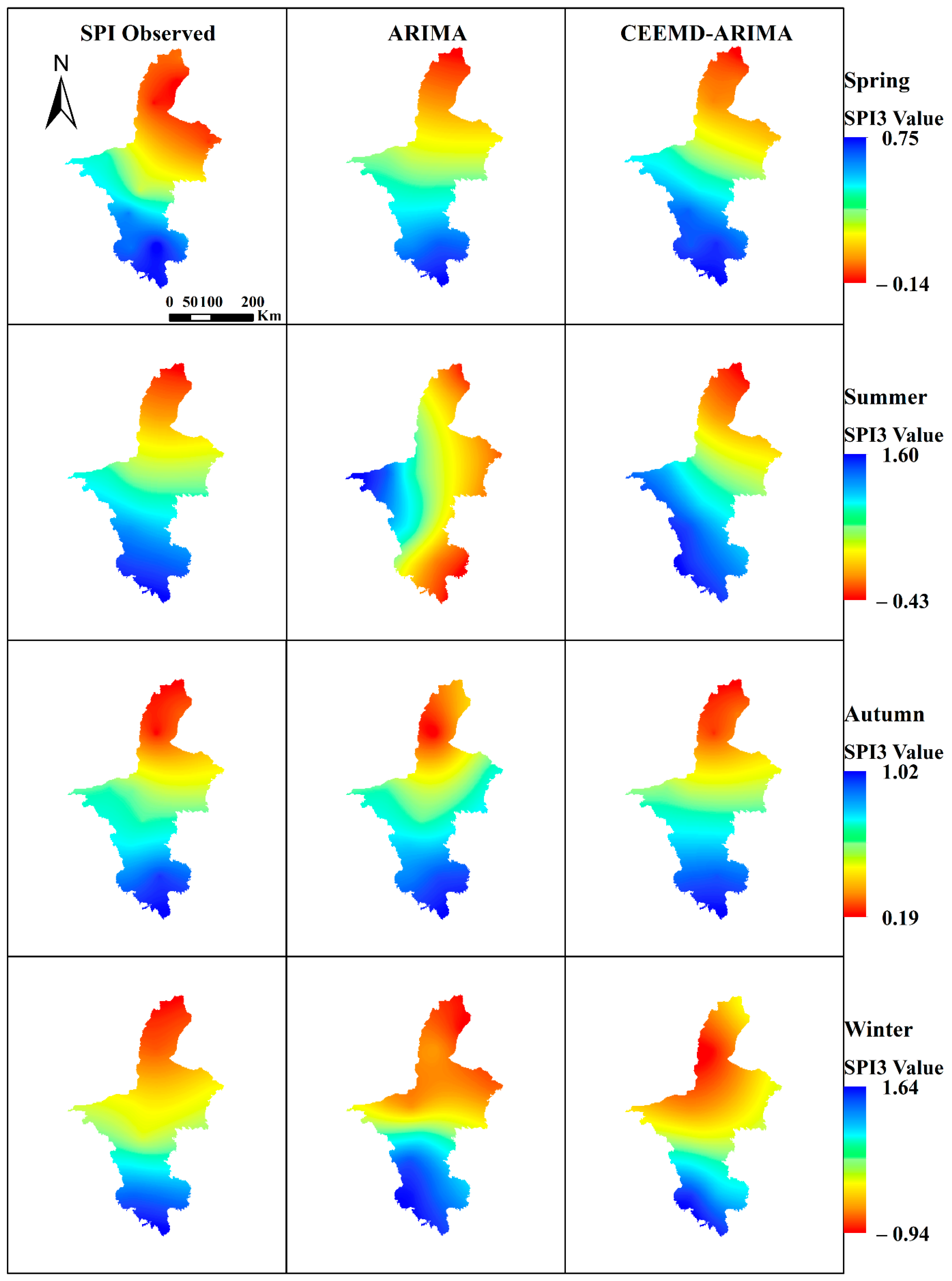
- The ARIMA model had the lowest prediction accuracy on the 1-month time scale and the highest on the 24-month time scale. At the same time scales, the prediction accuracy of the CEEMD–ARIMA model was higher than that of the ARIMA model. According to the visual display of the forecast results of the 3-month time scale, in the seasons of spring, summer, autumn, and winter, the drought conditions predicted by CEEMD–ARIMA were more consistent with the actual conditions.
- (3)
- The drought prediction of CEEMD–ARIMA was approximately consistent with the China Meteorological Network records, indicating that the combined model is suitable for drought prediction. The original sequence was decomposed by CEEMD, and then the decomposed sequence was predicted by the ARIMA model. Finally, the predicted values of each component were added together to obtain the final prediction result. The final prediction result had high precision. According to the prediction results, the CEEMD–ARIMA model obtains higher prediction accuracy than the ARIMA model at multiple time scales, meaning that the combined model can better fit the SPI sequence at different time scales.
Author Contributions
Funding
Institutional Review Board Statement
Informed Consent Statement
Data Availability Statement
Conflicts of Interest
References
- Fang, O.; Zhang, Q.B.; Vitasse, Y.; Zweifel, R.; Cherubini, P. The Frequency and Severity of Past Droughts Shape the Drought Sensitivity of Juniper Trees on the Tibetan Plateau. For. Ecol. Manag. 2021, 486, 118968. [Google Scholar] [CrossRef]
- Xu, Y.; Zhang, X.; Wang, X.; Hao, Z.; Singh, V.P.; Hao, F. Propagation from Meteorological Drought to Hydrological Drought under the Impact of Human Activities: A Case Study in Northern China. J. Hydrol. 2019, 579, 124147. [Google Scholar] [CrossRef]
- Khan, R.; Gilani, H. Global Drought Monitoring with Drought Severity Index (DSI) Using Google Earth Engine. Theor. Appl. Climatol. 2021, 146, 411–427. [Google Scholar] [CrossRef]
- Esfahanian, E.; Nejadhashemi, A.P.; Abouali, M.; Adhikari, U.; Zhang, Z.; Daneshvar, F.; Herman, M.R. Development and Evaluation of a Comprehensive Drought Index. J. Environ. Manag. 2017, 185, 31–43. [Google Scholar] [CrossRef] [PubMed] [Green Version]
- Araneda-Cabrera, R.J.; Bermúdez, M.; Puertas, J. Benchmarking of Drought and Climate Indices for Agricultural Drought Monitoring in Argentina. Sci. Total Environ. 2021, 790, 148090. [Google Scholar] [CrossRef]
- Liu, Q.; Zhang, G.; Ali, S.; Wang, X.; Wang, G.; Pan, Z.; Zhang, J. SPI-Based Drought Simulation and Prediction Using ARMA-GARCH Model. Appl. Math. Comput. 2019, 355, 96–107. [Google Scholar] [CrossRef]
- Zhang, J.; Sun, F.; Lai, W.; Lim, W.H.; Liu, W.; Wang, T.; Wang, P. Attributing Changes in Future Extreme Droughts Based on PDSI in China. J. Hydrol. 2019, 573, 607–615. [Google Scholar] [CrossRef]
- Yuan, X.; Jian, J.; Jiang, G. Spatiotemporal Variation of Precipitation Regime in China from 1961 to 2014 from the Standardized Precipitation Index. ISPRS Int. J. Geo-Inf. 2016, 5, 194. [Google Scholar] [CrossRef] [Green Version]
- Asadi Zarch, M.A.; Sivakumar, B.; Sharma, A. Droughts in a Warming Climate: A Global Assessment of Standardized Precipitation Index (SPI) and Reconnaissance Drought Index (RDI). J. Hydrol. 2015, 526, 183–195. [Google Scholar] [CrossRef]
- Bai, J.J.; Yu, Y.; Di, L. Comparison between TVDI and CWSI for Drought Monitoring in the Guanzhong Plain, China. J. Integr. Agric. 2017, 16, 389–397. [Google Scholar] [CrossRef] [Green Version]
- Shi, B.; Zhu, X.; Hu, Y.; Yang, Y. Drought Characteristics of Henan Province in 1961-2013 Based on Standardized Precipitation Evapotranspiration Index. J. Geogr. Sci. 2017, 27, 311–325. [Google Scholar] [CrossRef]
- Sivakumar, V.L.; Ramalakshmi, M.; Krishnappa, R.R.; Manimaran, J.C.; Paranthaman, P.K.; Priyadharshini, B.; Periyasami, R.K. An Integration of Geospatial Technology and Standard Precipitation Index (SPI) for Drought Vulnerability Assessment for a Part of Namakkal District, South India. Mater. Today Proc. 2020, 33, 1206–1211. [Google Scholar] [CrossRef]
- De Oliveira-Júnior, J.F.; de Gois, G.; de Bodas Terassi, P.M.; da Silva Junior, C.A.; Blanco, C.J.C.; Sobral, B.S.; Gasparini, K.A.C. Drought Severity Based on the SPI Index and Its Relation to the ENSO and PDO Climatic Variability Modes in the Regions North and Northwest of the State of Rio de Janeiro—Brazil. Atmos. Res. 2018, 212, 91–105. [Google Scholar] [CrossRef]
- Wu, J.; Chen, X.; Yao, H.; Zhang, D. Multi-Timescale Assessment of Propagation Thresholds from Meteorological to Hydrological Drought. Sci. Total Environ. 2021, 765, 144232. [Google Scholar] [CrossRef] [PubMed]
- Xu, Y.; Zhang, X.; Hao, Z.; Singh, V.P.; Hao, F. Characterization of Agricultural Drought Propagation over China Based on Bivariate Probabilistic Quantification. J. Hydrol. 2021, 598, 126194. [Google Scholar] [CrossRef]
- Łabȩdzki, L. Estimation of Local Drought Frequency in Central Poland Using the Standardized Precipitation Index SPI. Irrig. Drain. 2007, 56, 67–77. [Google Scholar] [CrossRef]
- Hao, Z.; Hao, F.; Xia, Y.; Singh, V.P.; Hong, Y.; Shen, X.; Ouyang, W. A Statistical Method for Categorical Drought Prediction Based on NLDAS-2. J. Appl. Meteorol. Climatol. 2016, 55, 1049–1061. [Google Scholar] [CrossRef]
- Khan, M.M.H.; Muhammad, N.S.; El-Shafie, A. Wavelet Based Hybrid ANN-ARIMA Models for Meteorological Drought Forecasting. J. Hydrol. 2020, 590, 125380. [Google Scholar] [CrossRef]
- Han, P.; Wang, P.X.; Zhang, S.Y.; Zhu, D.H. Drought Forecasting Based on the Remote Sensing Data Using ARIMA Models. Math. Comput. Model. 2010, 51, 1398–1403. [Google Scholar] [CrossRef]
- Shatanawi, K.; Rahbeh, M.; Shatanawi, M. Characterizing, Monitoring and Forecasting of Drought in Jordan River Basin. J. Water Resour. Prot. 2013, 5, 1192–1202. [Google Scholar] [CrossRef] [Green Version]
- Fung, K.F.; Huang, Y.F.; Koo, C.H. Coupling Fuzzy–SVR and Boosting–SVR Models with Wavelet Decomposition for Meteorological Drought Prediction. Environ. Earth Sci. 2019, 78, 1–18. [Google Scholar] [CrossRef]
- Xu, D.; Zhang, Q.; Ding, Y.; Huang, H. Application of a Hybrid Arima–Svr Model Based on the Spi for the Forecast of Drought—A Case Study in Henan Province, China. J. Appl. Meteorol. Climatol. 2020, 59, 1239–1259. [Google Scholar] [CrossRef] [Green Version]
- Han, P.; Wang, P.; Tian, M.; Zhang, S.; Liu, J.; Zhu, D. Application of the ARIMA Models in Drought Forecasting Using the Standardized Precipitation Index. IFIP Adv. Inf. Commun. Technol. 2013, 392, 352–358. [Google Scholar] [CrossRef] [Green Version]
- Özger, M.; Başakın, E.E.; Ekmekcioğlu, Ö.; Hacısüleyman, V. Comparison of Wavelet and Empirical Mode Decomposition Hybrid Models in Drought Prediction. Comput. Electron. Agric. 2020, 179, 105851. [Google Scholar] [CrossRef]
- Libanda, B.; Nkolola, N.B. An Ensemble Empirical Mode Decomposition of Consecutive Dry Days in the Zambezi Riparian Region: Implications for Water Management. Phys. Chem. Earth 2022, 126, 103147. [Google Scholar] [CrossRef]
- Tang, L.; Dai, W.; Yu, L.; Wang, S. A Novel CEEMD-Based Eelm Ensemble Learning Paradigm for Crude Oil Price Forecasting. Int. J. Inf. Technol. Decis. Mak. 2015, 14, 141–169. [Google Scholar] [CrossRef]
- Niu, M.; Wang, Y.; Sun, S.; Li, Y. A Novel Hybrid Decomposition-and-Ensemble Model Based on CEEMD and GWO for Short-Term PM2.5 Concentration Forecasting. Atmos. Environ. 2016, 134, 168–180. [Google Scholar] [CrossRef]
- Li, J.; He, K.; Tan, M.; Cheng, X. An Adaptive CEEMD-ANN Algorithm and Its Application in Pneumatic Conveying Flow Pattern Identification. Flow Meas. Instrum. 2021, 77, 101860. [Google Scholar] [CrossRef]
- Mckee, T.B.; Doesken, N.J.; Kleist, J. The relationship of drought frequency and duration to time scales. In Proceedings of the 8th Conference on Applied Climatology, Anaheim, CA, USA, 17–22 January 1993; pp. 179–184. [Google Scholar]
- Belayneh, A.; Adamowski, J.; Khalil, B.; Ozga-Zielinski, B. Long-Term SPI Drought Forecasting in the Awash River Basin in Ethiopia Using Wavelet Neural Networks and Wavelet Support Vector Regression Models. J. Hydrol. 2014, 508, 418–429. [Google Scholar] [CrossRef]
- Lloyd-Hughes, B.; Saunders, M.A. A Drought Climatology for Europe. Int. J. Climatol. 2002, 22, 1571–1592. [Google Scholar] [CrossRef]
- Javed, T.; Li, Y.; Rashid, S.; Li, F.; Hu, Q.; Feng, H.; Chen, X.; Ahmad, S.; Liu, F.; Pulatov, B. Performance and Relationship of Four Different Agricultural Drought Indices for Drought Monitoring in China’s Mainland Using Remote Sensing Data. Sci. Total Environ. 2021, 759, 143530. [Google Scholar] [CrossRef]
- Box, G.E.P.; Jenkins, G.M.; Reinsel, G.C.; Ljung, G.M. Time Series Analysis: Forecasting and Control; Holden-Day: San Francisco, CA, USA, 1976. [Google Scholar]
- Yeh, J.R.; Shieh, J.S.; Huang, N.E. Complementary Ensemble Empirical Mode Decomposition: A Novel Noise Enhanced Data Analysis Method. Adv. Adapt. Data Anal. 2010, 2, 135–156. [Google Scholar] [CrossRef]
- Mehdizadeh, S.; Ahmadi, F.; Kozekalani Sales, A. Modelling Daily Soil Temperature at Different Depths via the Classical and Hybrid Models. Meteorol. Appl. 2020, 27, 1–15. [Google Scholar] [CrossRef]
- Esmaeili-Gisavandani, H.; Farajpanah, H.; Adib, A.; Kisi, O.; Riyahi, M.M.; Lotfirad, M.; Salehpoor, J. Evaluating Ability of Three Types of Discrete Wavelet Transforms for Improving Performance of Different ML Models in Estimation of Daily-Suspended Sediment Load. Arab. J. Geosci. 2022, 15, 1–13. [Google Scholar] [CrossRef]
- Ahmadi, F.; Mehdizadeh, S.; Nourani, V. Improving the Performance of Random Forest for Estimating Monthly Reservoir Inflow via Complete Ensemble Empirical Mode Decomposition and Wavelet Analysis. Stoch. Environ. Res. Risk Assess. 2022, 1–16. [Google Scholar] [CrossRef]
- Adib, A.; Zaerpour, A.; Kisi, O.; Lotfirad, M. A Rigorous Wavelet-Packet Transform to Retrieve Snow Depth from SSMIS Data and Evaluation of Its Reliability by Uncertainty Parameters. Water Resour. Manag. 2021, 35, 2723–2740. [Google Scholar] [CrossRef]
- Liu, M.D.; Ding, L.; Bai, Y.L. Application of Hybrid Model Based on Empirical Mode Decomposition, Novel Recurrent Neural Networks and the ARIMA to Wind Speed Prediction. Energy Convers. Manag. 2021, 233, 113917. [Google Scholar] [CrossRef]
- Sun, H.; Zhai, W.; Wang, Y.; Yin, L.; Zhou, F. Privileged Information-Driven Random Network Based Non-Iterative Integration Model for Building Energy Consumption Prediction. Appl. Soft Comput. 2021, 108, 107438. [Google Scholar] [CrossRef]
- Wu, C.; Wang, J.; Chen, X.; Du, P.; Yang, W. A Novel Hybrid System Based on Multi-Objective Optimization for Wind Speed Forecasting. Renew. Energy 2020, 146, 149–165. [Google Scholar] [CrossRef]
- Zhang, X.; Wu, X.; He, S.; Zhao, D. Precipitation Forecast Based on CEEMD-LSTM Coupled Model. Water Supply 2021, 21, 4641–4657. [Google Scholar] [CrossRef]
- Ali, M.; Prasad, R.; Xiang, Y.; Yaseen, Z.M. Complete Ensemble Empirical Mode Decomposition Hybridized with Random Forest and Kernel Ridge Regression Model for Monthly Rainfall Forecasts. J. Hydrol. 2020, 584, 124647. [Google Scholar] [CrossRef]
- Zhang, Y.; Yan, B.; Aasma, M. A Novel Deep Learning Framework: Prediction and Analysis of Financial Time Series Using CEEMD and LSTM. Expert Syst. Appl. 2020, 159, 113609. [Google Scholar] [CrossRef]
- Rezaei, H.; Faaljou, H.; Mansourfar, G. Stock Price Prediction Using Deep Learning and Frequency Decomposition. Expert Syst. Appl. 2021, 169, 114332. [Google Scholar] [CrossRef]


| Station Number | Station Name | Longitude/°E | Latitude/°N | Altitude/m |
|---|---|---|---|---|
| 53519 | Huinong | 106.46 | 39.13 | 1092.5 |
| 53810 | Tongxin | 105.54 | 36.58 | 1339.3 |
| 53903 | Xiji | 105.43 | 35.58 | 1916.5 |
| SPI Value | Category |
|---|---|
| SPI > −0.5 | No drought |
| −1.0 < SPI ≤ −0.5 | Mild drought |
| −1.5 < SPI ≤ −1.0 | Moderate drought |
| −2.0 < SPI ≤ −1.5 | Severe drought |
| SPI ≤ −2.0 | Extreme drought |
| Example Stations | SPI Series | ADF | Critical Value | p-Value | ||
|---|---|---|---|---|---|---|
| 1% | 5% | 10% | ||||
| Huinong | SPI1 | −20.0550 | −3.4418 | −2.8666 | −2.5694 | 0.0000 |
| SPI3 | −9.6732 | −3.4419 | −2.8666 | −2.5695 | 1.2610 × 10⁻¹⁶ | |
| SPI6 | −6.9028 | −3.4420 | −2.8667 | −2.5695 | 1.2693 × 10⁻⁹ | |
| SPI9 | −5.3241 | −3.4423 | −2.8668 | −2.5696 | 4.8806 × 10⁻⁶ | |
| SPI12 | −4.7455 | −3.4423 | −2.8668 | −2.5696 | 6.9075 × 10⁻⁵ | |
| SPI24 | −4.1882 | −3.4423 | −2.8668 | −2.5696 | 0.0007 | |
| Tongxin | SPI1 | −21.6155 | −3.4418 | −2.8666 | −2.5694 | 0.0000 |
| SPI3 | −9.6077 | −3.4419 | −2.8666 | −2.5695 | 1.8469 × 10⁻¹⁶ | |
| SPI6 | −6.7922 | −3.4420 | −2.8667 | −2.5695 | 2.3486 × 10⁻⁹ | |
| SPI9 | −4.9104 | −3.4423 | −2.8668 | −2.5696 | 3.3288 × 10⁻⁵ | |
| SPI12 | −4.4071 | −3.4423 | −2.8668 | −2.5696 | 0.0003 | |
| SPI24 | −3.7087 | −3.4423 | −2.8668 | −2.5696 | 0.0040 | |
| Xiji | SPI1 | −22.0945 | −3.4418 | −2.8666 | −2.5694 | 0.0000 |
| SPI3 | −10.7739 | −3.4419 | −2.8666 | −2.5695 | 2.3469 × 10⁻¹⁹ | |
| SPI6 | −7.3216 | −3.4420 | −2.8667 | −2.5695 | 1.1900 × 10⁻¹⁰ | |
| SPI9 | −4.1113 | −3.4423 | −2.8668 | −2.5696 | 0.0009 | |
| SPI12 | −3.4578 | −3.4422 | −2.8668 | −2.5696 | 0.0091 | |
| SPI24 | −3.3257 | −3.4423 | −2.8668 | −2.5696 | 0.0138 | |
| Example Stations | SPI Series | Model Select | AIC | BIC | Model Order Estimation |
|---|---|---|---|---|---|
| Huinong | SPI1 | ARMA | 1826.071 | 1839.804 | ARMA (1, 0) |
| SPI3 | ARMA | 1631.778 | 1650.079 | ARMA (0, 2) | |
| SPI6 | ARMA | 1398.692 | 1412.404 | ARMA (1, 0) | |
| SPI9 | ARMA | 1026.739 | 1045.006 | ARMA (1, 0) | |
| SPI12 | ARMA | 538.884 | 579.946 | ARMA (5, 2) | |
| SPI24 | ARMA | 64.999 | 87.725 | ARMA (3, 0) | |
| Tongxin | SPI1 | ARMA | 1937.225 | 1950.959 | ARMA (1, 0) |
| SPI3 | ARMA | 1593.929 | 1612.230 | ARMA (0, 2) | |
| SPI6 | ARMA | 1302.638 | 1343.776 | ARMA (5, 2) | |
| SPI9 | ARMA | 957.282 | 970.982 | ARMA (1, 0) | |
| SPI12 | ARMA | 536.069 | 586.256 | ARMA (7, 2) | |
| SPI24 | ARMA | 43.954 | 62.136 | ARMA (2, 0) | |
| Xiji | SPI1 | ARMA | 2012.614 | 2026.347 | ARMA (0, 1) |
| SPI3 | ARMA | 1628.778 | 1647.078 | ARMA (0, 2) | |
| SPI6 | ARMA | 1453.959 | 1472.242 | ARMA (2, 0) | |
| SPI9 | ARMA | 1061.371 | 1075.071 | ARMA (1, 0) | |
| SPI12 | ARMA | 575.482 | 616.544 | ARMA (5, 2) | |
| SPI24 | ARMA | 31.131 | 62.949 | ARMA (3, 2) |
| SPI Series | Decompose Results | Model Select | Model Order Estimation |
|---|---|---|---|
| SPI3 | IMF1 | ARMA | ARMA (1, 1) |
| IMF2 | ARMA | ARMA (2, 5) | |
| IMF3 | ARMA | ARMA (4, 2) | |
| IMF4 | ARMA | ARMA (4, 5) | |
| IMF5 | ARMA | ARMA (4, 6) | |
| IMF6 | ARMA | ARMA (2, 1) | |
| IMF7 | ARIMA | ARIMA (4, 1, 1) | |
| Res | ARIMA | ARIMA (3, 1, 1) |
| Example Stations | SPI Series | Model | Training | Testing | ||||||||
|---|---|---|---|---|---|---|---|---|---|---|---|---|
| MAE | RMSE | NSE | KGE | WI | MAE | RMSE | NSE | KGE | WI | |||
| Huinong | SPI1 | ARIMA | 0.634 | 0.850 | −31.759 | −3.881 | 0.204 | 0.667 | 0.892 | −48.453 | −4.992 | 0.150 |
| CEEMD–ARIMA | 0.459 | 0.580 | −0.020 | 0.440 | 0.830 | 0.465 | 0.596 | −0.058 | 0.420 | 0.817 | ||
| SPI3 | ARIMA | 0.535 | 0.708 | −0.544 | 0.284 | 0.750 | 0.549 | 0.723 | −0.663 | −0.250 | 0.730 | |
| CEEMD–ARIMA | 0.393 | 0.502 | 0.497 | 0.654 | 0.894 | 0.407 | 0.526 | 0.448 | 0.632 | 0.886 | ||
| SPI6 | ARIMA | 0.429 | 0.609 | 0.363 | 0.643 | 0.867 | 0.440 | 0.618 | −0.013 | 0.452 | 0.783 | |
| CEEMD–ARIMA | 0.244 | 0.312 | 0.860 | 0.886 | 0.962 | 0.250 | 0.321 | 0.808 | 0.861 | 0.954 | ||
| SPI9 | ARIMA | 0.304 | 0.434 | 0.711 | 0.816 | 0.934 | 0.315 | 0.460 | 0.384 | 0.671 | 0.850 | |
| CEEMD–ARIMA | 0.143 | 0.188 | 0.927 | 0.893 | 0.981 | 0.150 | 0.199 | 0.906 | 0.876 | 0.977 | ||
| SPI12 | ARIMA | 0.219 | 0.348 | 0.883 | 0.921 | 0.972 | 0.226 | 0.363 | 0.604 | 0.783 | 0.896 | |
| CEEMD–ARIMA | 0.125 | 0.186 | 0.925 | 0.927 | 0.982 | 0.129 | 0.194 | 0.884 | 0.923 | 0.972 | ||
| SPI24 | ARIMA | 0.149 | 0.233 | 0.939 | 0.953 | 0.985 | 0.157 | 0.248 | 0.670 | 0.831 | 0.911 | |
| CEEMD–ARIMA | 0.067 | 0.087 | 0.957 | 0.978 | 0.990 | 0.069 | 0.090 | 0.954 | 0.972 | 0.989 | ||
| Tongxin | SPI1 | ARIMA | 0.711 | 0.909 | −87.660 | −7.274 | 0.127 | 0.724 | 0.918 | −100.523 | −8.116 | 0.115 |
| CEEMD–ARIMA | 0.452 | 0.557 | 0.415 | 0.133 | 0.879 | 0.466 | 0.574 | 0.374 | 0.130 | 0.868 | ||
| SPI3 | ARIMA | 0.578 | 0.729 | −0.286 | 0.360 | 0.783 | 0.606 | 0.740 | −0.395 | 0.133 | 0.758 | |
| CEEMD–ARIMA | 0.343 | 0.416 | 0.787 | 0.377 | 0.952 | 0.349 | 0.424 | 0.750 | 0.369 | 0.944 | ||
| SPI6 | ARIMA | 0.437 | 0.588 | 0.489 | 0.704 | 0.890 | 0.467 | 0.626 | 0.357 | 0.499 | 0.859 | |
| CEEMD–ARIMA | 0.207 | 0.275 | 0.934 | 0.553 | 0.985 | 0.224 | 0.296 | 0.894 | 0.541 | 0.974 | ||
| SPI9 | ARIMA | 0.323 | 0.472 | 0.731 | 0.791 | 0.938 | 0.325 | 0.482 | 0.632 | 0.783 | 0.915 | |
| CEEMD–ARIMA | 0.138 | 0.181 | 0.960 | 0.804 | 0.991 | 0.142 | 0.187 | 0.952 | 0.797 | 0.988 | ||
| SPI12 | ARIMA | 0.235 | 0.336 | 0.873 | 0.916 | 0.969 | 0.239 | 0.341 | 0.823 | 0.853 | 0.957 | |
| CEEMD–ARIMA | 0.090 | 0.122 | 0.984 | 0.967 | 0.996 | 0.096 | 0.130 | 0.976 | 0.962 | 0.994 | ||
| SPI24 | ARIMA | 0.159 | 0.247 | 0.937 | 0.956 | 0.985 | 0.172 | 0.253 | 0.921 | 0.944 | 0.980 | |
| CEEMD–ARIMA | 0.062 | 0.079 | 0.996 | 0.975 | 0.999 | 0.065 | 0.083 | 0.992 | 0.972 | 0.998 | ||
| Xiji | SPI1 | ARIMA | 0.782 | 0.961 | −116.898 | −10.640 | 0.237 | 0.825 | 1.036 | −126.675 | −36.326 | 0.224 |
| CEEMD–ARIMA | 0.570 | 0.706 | 0.269 | 0.205 | 0.846 | 0.584 | 0.739 | 0.256 | 0.182 | 0.831 | ||
| SPI3 | ARIMA | 0.574 | 0.731 | −0.313 | 0.370 | 0.774 | 0.649 | 0.820 | −0.487 | −0.528 | 0.752 | |
| CEEMD–ARIMA | 0.391 | 0.481 | 0.717 | 0.794 | 0.939 | 0.407 | 0.508 | 0.689 | 0.776 | 0.930 | ||
| SPI6 | ARIMA | 0.492 | 0.657 | 0.332 | 0.529 | 0.877 | 0.547 | 0.670 | 0.313 | 0.262 | 0.869 | |
| CEEMD–ARIMA | 0.235 | 0.297 | 0.930 | 0.842 | 0.984 | 0.247 | 0.309 | 0.923 | 0.835 | 0.981 | ||
| SPI9 | ARIMA | 0.346 | 0.490 | 0.711 | 0.768 | 0.936 | 0.412 | 0.576 | 0.696 | 0.482 | 0.933 | |
| CEEMD–ARIMA | 0.211 | 0.279 | 0.948 | 0.934 | 0.988 | 0.221 | 0.291 | 0.940 | 0.923 | 0.985 | ||
| SPI12 | ARIMA | 0.229 | 0.354 | 0.890 | 0.888 | 0.980 | 0.245 | 0.377 | 0.890 | 0.625 | 0.974 | |
| CEEMD–ARIMA | 0.102 | 0.136 | 0.987 | 0.937 | 0.997 | 0.107 | 0.141 | 0.987 | 0.921 | 0.997 | ||
| SPI24 | ARIMA | 0.158 | 0.233 | 0.950 | 0.753 | 0.989 | 0.188 | 0.285 | 0.949 | 0.514 | 0.988 | |
| CEEMD–ARIMA | 0.069 | 0.087 | 0.995 | 0.994 | 0.999 | 0.076 | 0.100 | 0.994 | 0.993 | 0.999 | ||
Publisher’s Note: MDPI stays neutral with regard to jurisdictional claims in published maps and institutional affiliations. |
© 2022 by the authors. Licensee MDPI, Basel, Switzerland. This article is an open access article distributed under the terms and conditions of the Creative Commons Attribution (CC BY) license (https://creativecommons.org/licenses/by/4.0/).
Share and Cite
Xu, D.; Ding, Y.; Liu, H.; Zhang, Q.; Zhang, D. Applicability of a CEEMD–ARIMA Combined Model for Drought Forecasting: A Case Study in the Ningxia Hui Autonomous Region. Atmosphere 2022, 13, 1109. https://doi.org/10.3390/atmos13071109
Xu D, Ding Y, Liu H, Zhang Q, Zhang D. Applicability of a CEEMD–ARIMA Combined Model for Drought Forecasting: A Case Study in the Ningxia Hui Autonomous Region. Atmosphere. 2022; 13(7):1109. https://doi.org/10.3390/atmos13071109
Chicago/Turabian StyleXu, Dehe, Yan Ding, Hui Liu, Qi Zhang, and De Zhang. 2022. "Applicability of a CEEMD–ARIMA Combined Model for Drought Forecasting: A Case Study in the Ningxia Hui Autonomous Region" Atmosphere 13, no. 7: 1109. https://doi.org/10.3390/atmos13071109